Pixel-level Tumor Margin Assessment of Surgical Specimen with Hyperspectral Imaging and Deep Learning Classification

Abstract

Surgery is a major treatment method for squamous cell carcinoma (SCC). During surgery, insufficient tumor margin may lead to local recurrence of cancer. Hyperspectral imaging (HSI) is a promising optical imaging technique for in vivo cancer detection and tumor margin assessment. In this study, a fully convolutional network (FCN) was implemented for tumor classification and margin assessment on hyperspectral images of SCC. The FCN was trained and validated with hyperspectral images of 25 ex vivo SCC surgical specimens from 20 different patients. The network was evaluated per patient and achieved pixel-level tissue classification with an average area under the curve (AUC) of 0.88, as well as 0.83 accuracy, 0.84 sensitivity, and 0.70 specificity across all the 20 patients. The 95% Hausdorff distance of assessed tumor margin in 17 patients was less than 2 mm, and the classification time of each tissue specimen took less than 10 seconds. The proposed methods can potentially facilitate intraoperative tumor margin assessment and improve surgical outcomes.

1. INTRODUCTION

Head and neck cancer is the sixth most common cancer worldwide [1–3]. Squamous cell carcinoma (SCC) takes more than 90% of the cancers of the upper aerodigestive tract of the head and neck [2]. Surgical resection has long been the major and standard treatment approach for head and neck SCC. One of the main challenges during surgical treatment is to obtain a high cure rate while realizing organ preservation [4–6]. Extension of tumor cells into the area around the resection, namely the surgical margin, may lead to local recurrences and second primary tumors that might subsequently worsen the surgical survival [2, 7, 8]. Therefore, an adequate margin, which varies from 5 mm to 20 mm [7, 9], is required during surgery.

Current intraoperative methods for surgeons to differentiate tumor and normal tissue are visual inspection, palpation, and frozen section [7, 8]. The resected tissue specimen is frozen and processed for an intraoperative pathologist consultant (IPC). Frozen section analysis (FSA) is the standard for tumor margin assessment. However, this procedure takes about 25~45 minutes per IPC, and it is susceptible to errors that occur during sampling and histological interpretation [9–13]. The incident rate of insufficient margin is 40%–50% [11, 12]. Thus, methods for fast and accurate surgical margin assessment are critical to improving surgical outcomes of head and neck cancer resection.

Hyperspectral imaging (HSI) is an optical imaging technique that is non-invasive, non-contact, and label-free. It expands surgeons’ vision from visible wavelength range to infrared and is able to utilize the rich spectral information of tissue, which reveals the change of tissue optical properties caused by the presence, progression, or regression of neoplasia [14]. HSI has been investigated for cancer detection in both in vivo and ex vivo tissues. A previous study of in vivo head and neck cancer detection using hyperspectral imaging has been performed by our group [15] on an animal model (N=12). A support vector machine (SVM) classifier using the tensor-based feature of spectral signature was implemented with 0.89 accuracy. Next, in vivo HSI and SVM classification were implemented on a mouse model of neoplastic 4NQU-induced tongue carcinogenesis, and the area under the curve (AUC) was 0.84 [16]. Later on, an ex vivo HSI head and neck cancer detection study in surgical specimens of 26 patients using SVM achieved 0.86 inter-patient accuracy [17]. In a recent study, our group [18] implemented deep learning classification using the Inception-v4 convolutional neural network (CNN) on 25×25-pixel patches. The network was trained and tested on a dataset of 102 SCC patients and achieved a patch-level AUC of 0.82.

In this study, U-Net architecture as a fully convolutional network (FCN) was implemented for tumor margin assessment in SCC surgical specimens. Compared to our previous studies [18] in which a trained fully-connected CNN was used for patch-level classification, this study aims to classify tumor and normal tissue in the images to generate pixel-level class labels for hyperspectral images. The robust experimental design and preliminary results of this study show the potential for our proposed method to aid fast and intraoperative surgical margin assessment.

2. METHODS

2.1. Hyperspectral Dataset of Head and Neck SCC Patients

The hyperspectral image dataset has been reported in our previous work [18]. Surgical specimens of head and neck SCC were collected when HNSCC patients underwent routine surgery. Hyperspectral images of the fresh ex-vivo surgical specimens were captured for the cancer detection study. For each patient, three specimens were collected, containing the primary tumor (T), normal tissue (N), and tumor-normal margin (TN), respectively. In this study, we used hyperspectral images of 25 conventional head and neck SCC specimens from 20 different patients. The specimens were from the larynx (22 specimens from 17 patients) and hypopharynx (3 specimens from 3 patients). Only the images of tumor-normal margin specimens were utilized for margin assessment.

The hyperspectral images were captured with a Maestro spectral imaging system (Perkin Elmer Inc., Waltham, Massachusetts). The system contained a liquid crystal tunable filter for spectral scanning over 91 wavelength bands from 450 nm to 900 nm with a 5 nm increment, and a 16-bit charge-coupled device (CCD) to capture two-dimensional grayscale images at each wavelength band. The spatial size of the hyperspectral images field of view (FOV) varies from 6.4 mm × 6.4 mm to 19.2 mm × 16 mm with a median size of 12.8 mm × 9.6 mm, and the specimen-level resolution is 25 um per pixel [18].

2.2. Data Preparation

After image acquisition, the ex vivo surgical specimens were inked, formalin fixed, and paraffin embedded. The top section of each specimen was obtained using a microtome, stained with hematoxylin and eosin (H&E), and digitalized using whole-slide scanning at 40× magnification [18]. A board-certified pathologist annotated the digital histology images to outline the cancerous and normal areas, then the histological ground truth was registered to the gross-level hyperspectral image using a deformable registration pipeline [19] and served as the gold standard.

Hyperspectral images were firstly calibrated with a white reference image and a dark reference image to obtain the normalized reflectance of the tissue specimens. Then, image patches were generated from the hyperspectral images using a sliding window. In this study, we trained the network with large image patches, because we had a relatively small dataset, and generating patches from the images could provide adequate training data for the network. In addition, we tried to have more patches for each specimen even the smallest one, so as to ensure enough training iterations that make the moving average and variance of the batch normalization layers in our network coverage. Therefore, we used a sliding window with strides of five pixels for small SCC specimens, and a sliding window with strides of 25 pixels for large specimens. The dimension of the generated patches was 256 pixels by 256 pixels by 91 bands. For the training data, only patches containing the tumor-normal margin were used to train the network, while the patches with only-tumor or only-normal tissue were not used in the training process. For each patient, we randomly selected an equal number (N=80) of patches of the tumor-normal margin to avoid model overfitting to specific patients caused by unbalanced patch numbers.

Except for the patches generated from a few hyperspectral images that included very little tumor or normal tissue, the number of tumor pixels and normal pixels in the training patches were as balanced as possible. Due to the limited size and irregular shape of the tissue, most patches contain background pixels, which have very different spectra from tissue pixels. The percentage of tissue pixels in each patch also varies because of the different sizes and shapes of specimens. Each patch was augmented eight times by rotating and reflecting before training. Figure 1 shows an example of a generated patch from the hyperspectral image of the SCC specimen.

Figure 1.

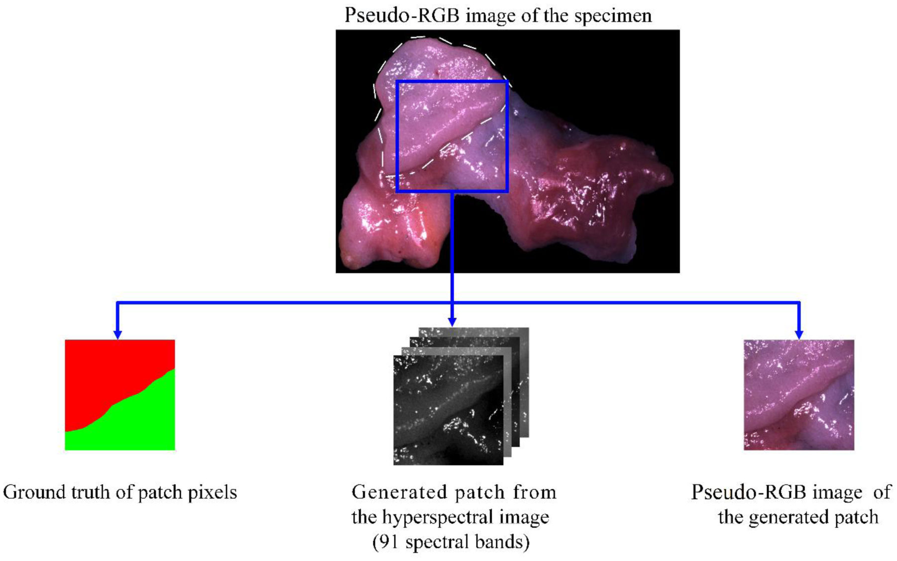
Illustration of the generated HSI patch and pseudo-RGB patch from the tumor-normal margin of an SCC specimen. The tumor is shown with a dashed contour in the pseudo-RGB image.

Due to the absence of the original RGB images of the specimens, we generated pseudo-RGB patches for each HSI patch, as also shown in Figure 1, and used the pseudo-RGB patches to train and validate the same network as HSI, in order to evaluate the usefulness of HSI compared to RGB. We used a customized HSI-to-RGB transformation, which is made up of several cosine functions and is close to the light response of the human eye, as has been described in our previous study [20]. However, due to the difference in the spectral range of hyperspectral imaging systems, we slightly modified the magnitudes of three channels to make the synthesized RGB images close to the real color.

2.3. Fully Convolutional Neural Network

A two-dimensional fully convolutional network based on the U-Net architecture [21] was implemented using Keras with a Tensorflow backend. The hyperspectral patches discussed in the previous section were utilized to train and validate the U-Net on a Titan XP NVIDIA GPU. The three-level U-Net shown in Figure 2 contains 10 standard convolutional layers, each of which was followed by a batch normalization layer [22] and ReLU activation. The kernel size of the convolutional layers in the first level was 5×5, while the kernel size of other standard convolutional layers was 3×3. The optimizer was Adam [23] with a learning rate of 5×10⁻⁵. The network was trained with a batch size of 12 for 6 to 12 epochs depending on how fast the validation accuracy stopped increasing. All convolutional layers were initialized with Xavier kernel initializer. L2 regularization [24] with an L2 constant of 10⁻⁷ was applied for each convolutional layer, and dropout [25] with the dropout ratio of 15% was applied after each block of convolutional layers. For loss function, we tried categorical cross-entropy and Dice coefficient-based loss [26]. Both loss functions had comparable performance and finally, categorical cross-entropy was selected as the loss function. The FCN that was trained using the pseudo-RGB patches had the same architecture and hyperparameters as the one trained with HSI patches, except that the size of the input layer was 256×256×3.

Figure 2.

The three-level U-Net architecture with 10 standard convolutional layers.

Due to the small size of the dataset used in this study, we created training and validation cohort of patches. For both FCNs (HSI and pseudo-RGB), we implemented 10-fold cross-validation. For each fold, the images of 18 patients (11520 patches in total) were used for training and the images of two patients (1280 patches in total) were used for validation. So, all patient data have been used for validation but in different folds. The patches from the same patient were never used in both training and validation at the same time. Moreover, the data partition for both FCNs was exactly the same to avoid the bias of comparison between two networks. The FCNs were trained with labels of three classes, namely tumor, normal, and background. Later in the validation process, only the tissue (tumor and normal tissue) pixels were used for evaluation.

Besides this network, we also tried a three-level U-Net with half number of features and a four-level U-Net. The U-Net with fewer features had a worse training performance, and the deeper network was easily over-fitted to one class (either tumor or normal) when trained on a subset of the data. Moreover, in comparison to our previous work [18, 27], which used smaller patches of 25×25 pixels and more complicated network architecture (Inception-v4), our U-Net was able to achieve pixel-level classification with far less convolutional layers.

2.4. Evaluation Metrics

Although the network was trained with three classes of labels, we only used the pixels of tissue but not the background in each hyperspectral image for evaluation. In other words, we used only the pixels that are labeled as either tumor or normal tissue in ground truth to calculate the metrics. The reasons for not counting on the background pixels are: (1) background can be easily differentiated from tissue due to its distinct spectrum and it is hardly misclassified, and (2) background was not included in all patches.

In this study, we used pixel-level overall accuracy, sensitivity, and specificity to evaluate the classification performance, as shown in Equation (1–3). Overall accuracy is defined as the ratio of the number of correctly labeled tissue pixels to the total number of tissue pixels in the ground truth. Specificity and sensitivity are calculated from true positive (TP), true negative (TN), false positive (FP), and false negative (FN), where positive corresponds to tumor pixels and negative to normal tissue pixels. Specificity is the ratio of TN pixels to the normal pixels, while sensitivity is the ratio of TP pixels to the tumor pixels.

$$\mathit{\text{Overall accuracy}}=\frac{TP+TN}{TP+FP+TN+FN}$$ (1)

$$\mathit{\text{Sensitivity}}=\frac{TP}{TP+FN}$$ (2)

$$\mathit{\text{Specificity}}=\frac{TN}{TN+FP}$$ (3)

Because of the complex shape and variant area of tumor tissue in different images, the abovementioned metrics do not necessarily show how well the tumor margin is assessed. Therefore, we calculated the Hausdorff distance (HD) of each classified tumor region and used it as another evaluation metric. There are two versions of HD, namely the maximum HD and 95% HD. The maximum HD is defined as the maximum distance of a set to the nearest point in another set [28], which in this study is the maximum distance between the margin of the predicted tumor tissue and the margin of tumor tissue in the ground truth. However, maximum HD is subject to noise, thus the impact of a very small subset of the outliers may result in a very high HD and cause the bias of evaluation. Therefore, we used 95% HD, which is the 95^th percentile of the distances between boundary points in the predicted tumor region and the ground truth, as shown in Figure 3. The calculated 95% HD in pixel was transformed to and recorded in millimeters according to the spatial resolution of the image (25 μm/pixel).

Figure 3.

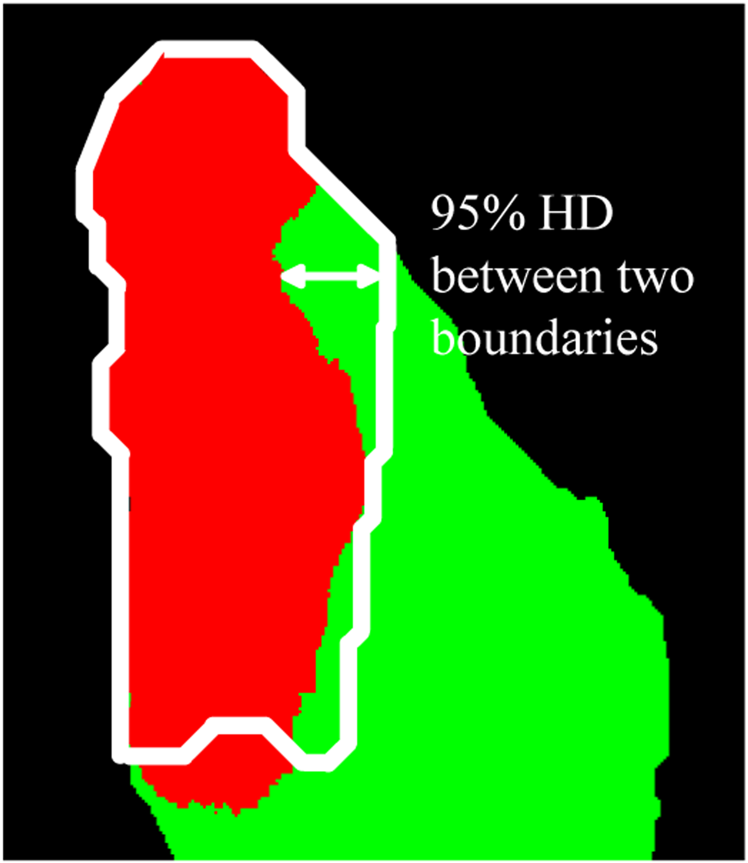
Evaluation of the marginal error using 95% Hausdorff distance. The white boundary indicates the ground truth of the tumor margin. The red region is the predicted tumor area while the green region is the predicted normal tissue.

3. RESULTS

The model was trained with only the patches that contain the tumor-normal margin, and for each patient, we used 80 patches. After the model was trained, we generated patches from the whole validation patient images using a sliding window with a stride of 128 pixels. All patches, regardless of how much tumor or normal tissue was included, were used for validation. The number of validation patches per specimen was one to ten, depending on the spatial size of the specimen. The generated validation patches were also eight times augmented by rotations and reflections. The classification time for all patches of one specimen was less than 10 seconds. After classifying all the patches, the average probability map for each patch was calculated across all eight augmented versions of the patch. Then, the probability map of the whole image was reconstructed by stitching all patches. For the overlapped areas, the average probabilities of the overlapped pixels were calculated and used. Afterwards, the accuracy, sensitivity, and specificity of the validation images were calculated using the probability map of the whole image. The optimal threshold levels based on the receiver operator characteristic (ROC) curve for validation data in different folds were 0.27 to 0.78. The same threshold was applied to all validation data in the same fold to generate classification labels.

We performed morphological opening and closing to the classification label images to smooth the tumor-normal margin. In a few cases, some pixels of the tumor tissue were classified as normal but were surrounded by tumor pixels, or some pixels in normal tissue were classified as tumor but surrounded by normal pixels. If the area of these misclassified pixels was smaller than 40 pixels×40 pixels (1 mm×1 mm), we filled this region with the same label as the surrounding pixels.

Otherwise, we kept the misclassified region. When calculating the 95% HD of tumor, the normal pixels that were classified as tumor were not used. Moreover, in some specimens, the edge of the tissue was very thin, which resulted in misclassification in the very narrow region surrounding the specimen. Therefore, we excluded 10 pixels, corresponding to 0.25 mm, at the edge of each specimen for performance evaluation.

The network was able to perform tissue classification in hyperspectral images of SCC surgical specimens with a pixel-level average AUC of 0.88 for the validation patients. The average accuracy, sensitivity, and specificity were 0.83, 0.84, and 0.70, respectively. However, there were two images (PT154 and PT172) where almost no margin was detected and the whole specimen was classified as one type. Similar situation also happened in the previous study using a patch-based CNN classification method [29]. Because the specimen of PT154 was classified as all normal with no predicted tumor pixels, we could not calculate the HD for this patient. For the specimen of PT172, which was classified as all tumor, the 95% HD was calculated between the boundary of the whole specimen and the tumor margin in the ground truth. If exclude these two images, the network could achieve an average AUC of 0.93, as well as 0.86 accuracy, 0.88 sensitivity, and 0.72 specificity. The maximum errors of assessed margin in the classified images of 18 patients (except PT154 and PT172) were smaller than 3 mm. In 17 out of 18 patients, the maximum margin error was smaller than 2 mm, among whom 9 patients had marginal error no larger than 1 mm. The median value of the 95% HD of 19 patients (except for PT154) was 1.03 mm. The classification results using the hyperspectral images of all patients are shown in Table 1.

Table 1.

The validation performance of each patient.

PT #	Organ*	No. of T pixels	No. of N pixels	AUC	Accuracy	Sensitivity	Specificity	95% HD (mm)
2	HYPO	27k	24k	0.95	0.82	0.82	0.81	1.41
27	LARN	53k	146k	0.89	0.93	0.93	0.93	1.24
29	LARN	79k	15k	0.99	0.95	0.95	0.98	1.03
30	LARN	52k	25k	0.82	0.73	0.82	0.52	2.00
41	LARN	21k	11k	0.91	0.81	0.86	0.72	1.00
43	HYPO	30k	18k	0.92	0.94	1.00	0.84	0.92
62	LARN	26k	37k	0.99	0.91	0.98	0.86	0.63
68	HYPO	77k	23k	0.99	0.91	0.88	0.99	1.24
74	LARN	67k	34k	0.98	0.88	0.99	0.67	1.77
110	LARN	5k	31k	0.77	0.80	0.10	0.94	1.5
127	LARN	44k	11k	0.99	0.97	0.99	0.90	0.43
134	LARN	38k	4k	0.99	0.90	0.91	0.84	0.62
137	LARN	32k	17k	0.82	0.63	0.96	0.10	3.00
154	LARN	15k	28k	0.2	0.65	0	1	--
166	LARN	52k	44k	0.88	0.70	0.91	0.53	1.50
172	LARN	28k	43k	0.76	0.40	1	0	7.17
174	LARN	95k	10k	0.98	0.92	0.97	0.39	0.97
184	LARN	50k	5k	0.97	0.90	0.97	0.20	1.00
187	LARN	20k	37k	0.98	0.93	0.89	0.95	0.71
188	LARN	29k	39k	0.88	0.83	0.92	0.77	1.00

^*HYPO: hypopharynx; LARN: larynx

The classification results of five different patients are shown in Figure 4. In the histology ground truth, the green annotation indicates the tumor region, while for the specimen shown in the second column in Figure 4, the whole slide was tumor except the region annotated in blue (dysplasia). The network was able to classify the tumor with a marginal error of less than 2 mm. Compared to the patch-based CNN in our previous study [18, 29], the U-Net model was less sensitive to glares with a better ability for high-precision margin assessment.

Figure 4.

Illustration of classification performance for five different patients (one per column): Pseudo-RGB images (1^st row) with the ground truth of tumor (white contour), histology ground truth (2^nd row), classification probability map using HSI (3^rd row), classification probability map using pseudo-RGB (4^th row), and predicted label generated from HSI probability map (5^th row, red for tumor and green for normal). White arrows show the glare pixels that were misclassified as tumor in the pseudo-RGB images, and black arrows show the regions that had very few glare pixels and were misclassified as normal. In the histology images (2^nd row), green contours indicate tumors, except the histology image in the second column, where the blue contour indicates dysplasia (normal) and the rest of the tissue is tumor.

The classification results using pseudo-RGB images were not as good as HSI in most specimens except for PT30. The network trained with pseudo-RGB patches got an average AUC of 0.84, as well as 0.71 accuracy, 0.80 sensitivity, and 0.64 specificity. The classification using pseudo-RGB patches was very much affected by the glares in the image. Tissue with most glares tended to be classified as tumor (white arrows in Figure 4) while tissue with very little glares was most likely to be classified as normal (black arrows in Figure 4). It is worth noting that the network was optimized for HSI, which might have caused some bias for the evaluation of RGB images. In the future, we will optimize the network for the pseudo-RGB images.

4. DISCUSSION AND CONCLUSION

In this study, a fully convolutional network model based on U-Net architecture was implemented and trained for tissue classification in hyperspectral images of ex vivo SCC surgical specimens. The model could provide pixel-level classification labels of the tumor and normal tissues with an average AUC of 0.88. The image classification for each specimen only takes 10 seconds. The whole process including image acquisition and processing can be done within several minutes, which is promising to provide fast tumor detection and high-precision margin assessment during the surgery. Compared to the time-consuming IPC, which requires the pathologist to carefully go over and manually annotate the whole slide, the proposed method only needs a pathologist to review the classification result for confirmation, which potentially saves much time during surgery. Although this work was based on a relatively small dataset and was evaluated using images of only two organs, it shows the ability of HSI to achieve accurate cancer detection. The comparison of HSI and RGB shows that the abundant spectral information within HSI can overcome certain limitations of human vision and provide insights into the tissue. In our future work, we will utilize a larger dataset of head and neck cancer specimens to train the network, and also include a testing group to better evaluate the performance of the network. In order to provide intraoperative image guidance, augmented reality-based systems will be developed, so that the classification results can be overlaid on the white-light image of the specimen and shown on a monitor or in a headset in real-time. The adoption and interpretation of HSI are easy for clinicians. Furthermore, since HSI is a non-contact, non-invasive, and label-free imaging method, it can be used any time on-demand during surgery. With the proposed classification method, HSI is promising to become an intraoperative tool. In conclusion, the robust experimental design and the preliminary testing results in this study illustrate the potential of our method to aid intraoperative surgical margin assessment and improve surgical outcomes.

REFERENCES

- [1].Vigneswaran N, and Williams MD, “Epidemiologic trends in head and neck cancer and aids in diagnosis,” Oral and Maxillofacial Surgery Clinics, 26(2), 123–141 (2014). [DOI] [PMC free article] [PubMed] [Google Scholar]
- [2].Leemans CR, Braakhuis BJ, and Brakenhoff RH, “The molecular biology of head and neck cancer,” Nature reviews cancer, 11(1), 9–22 (2011). [DOI] [PubMed] [Google Scholar]
- [3].Wissinger E, Griebsch I, Lungershausen J, Foster T, and Pashos CL, “The economic burden of head and neck cancer: a systematic literature review,” Pharmacoeconomics, 32(9), 865–882 (2014). [DOI] [PMC free article] [PubMed] [Google Scholar]
- [4].Marur S, and Forastiere AA, “Head and neck squamous cell carcinoma: update on epidemiology, diagnosis, and treatment.” 91, 386–396. [DOI] [PubMed] [Google Scholar]
- [5].Haddad RI, and Shin DM, “Recent advances in head and neck cancer,” New England Journal of Medicine, 359(11), 1143–1154 (2008). [DOI] [PubMed] [Google Scholar]
- [6].Argiris A, Karamouzis MV, Raben D, and Ferris RL, “Head and neck cancer,” The Lancet, 371(9625), 1695–1709 (2008). [DOI] [PMC free article] [PubMed] [Google Scholar]
- [7].Heidkamp J, Weijs WL, van Engen-van Grunsven AC, de Laak-de Vries I, Maas MC, Rovers MM, Fütterer JJ, Steens SC, and Takes RP, “Assessment of surgical tumor-free resection margins in fresh squamous-cell carcinoma resection specimens of the tongue using a clinical MRI system,” Head & Neck, (2020). [DOI] [PMC free article] [PubMed] [Google Scholar]
- [8].Calabrese L, Pietrobon G, Fazio E, Abousiam M, Awny S, Bruschini R, and Accorona R, “Anatomically-based transoral surgical approach to early-stage oral tongue squamous cell carcinoma,” Head & Neck, n/a(n/a), (2020). [DOI] [PubMed] [Google Scholar]
- [9].Hinni ML, Ferlito A, Brandwein-Gensler MS, Takes RP, Silver CE, Westra WH, Seethala RR, Rodrigo JP, Corry J, and Bradford CR, “Surgical margins in head and neck cancer: a contemporary review, ” Head & neck, 35(9), 1362–1370 (2013). [DOI] [PubMed] [Google Scholar]
- [10].Meier JD, Oliver DA, and Varvares MA, “Surgical margin determination in head and neck oncology: current clinical practice. The results of an International American Head and Neck Society Member Survey,” Head & Neck: Journal for the Sciences and Specialties of the Head and Neck, 27(11), 952–958 (2005). [DOI] [PubMed] [Google Scholar]
- [11].Sutton D, Brown J, Rogers SN, Vaughan E, and Woolgar J, “The prognostic implications of the surgical margin in oral squamous cell carcinoma,” International journal of oral and maxillofacial surgery, 32(1), 30–34 (2003). [DOI] [PubMed] [Google Scholar]
- [12].Kerker FA, Adler W, Brunner K, Moest T, Wurm MC, Nkenke E, Neukam FW, and von Wilmowsky C, “Anatomical locations in the oral cavity where surgical resections of oral squamous cell carcinomas are associated with a close or positive margin—a retrospective study,” Clinical oral investigations, 22(4), 1625–1630 (2018). [DOI] [PubMed] [Google Scholar]
- [13].Gandour-Edwards RF, Donald PJ, and Wiese DA, “Accuracy of intraoperative frozen section diagnosis in head and neck surgery: experience at a university medical center,” Head & neck, 15(1), 33–38 (1993). [DOI] [PubMed] [Google Scholar]
- [14].Ilhan B, Lin K, Guneri P, and Wilder-Smith P, “Improving Oral Cancer Outcomes with Imaging and Artificial Intelligence,” Journal of Dental Research, 99(3), 241–248 (2020). [DOI] [PMC free article] [PubMed] [Google Scholar]
- [15].Lu GL, Halig LM, Wang DS, Qin XL, Chen ZG, and Fei BW, “Spectral-spatial classification for noninvasive cancer detection using hyperspectral imaging,” Journal of Biomedical Optics, 19(10), (2014). [DOI] [PMC free article] [PubMed] [Google Scholar]
- [16].Lu G, Wang D, Qin X, Muller S, Wang X, Chen AY, Chen ZG, and Fei B, “Detection and delineation of squamous neoplasia with hyperspectral imaging in a mouse model of tongue carcinogenesis,” J Biophotonics, 11(3), (2018). [DOI] [PMC free article] [PubMed] [Google Scholar]
- [17].Lu G, Little JV, Wang X, Zhang H, Patel MR, Griffith CC, El-Deiry MW, Chen AY, and Fei B, “Detection of Head and Neck Cancer in Surgical Specimens Using Quantitative Hyperspectral Imaging,” Clin Cancer Res, 23(18), 5426–5436 (2017). [DOI] [PMC free article] [PubMed] [Google Scholar]
- [18].Halicek M, Dormer JD, Little JV, Chen AY, Myers L, Sumer BD, and Fei B, “Hyperspectral Imaging of Head and Neck Squamous Cell Carcinoma for Cancer Margin Detection in Surgical Specimens from 102 Patients Using Deep Learning,” Cancers (Basel), 11(9), (2019). [DOI] [PMC free article] [PubMed] [Google Scholar]
- [19].Halicek M, Little JV, Wang X, Chen ZG, Patel M, Griffith CC, El-Deiry MW, Saba NF, Chen AY, and Fei B, “Deformable Registration of Histological Cancer Margins to Gross Hyperspectral Images using Demons,” Proc SPIE Int Soc Opt Eng, 10581, (2018). [DOI] [PMC free article] [PubMed] [Google Scholar]
- [20].Ma L, Halicek M, Zhou X, Dormer J, and Fei B, “Hyperspectral microscopic imaging for automatic detection of head and neck squamous cell carcinoma using histologic image and machine learning.” 11320, 113200W. [DOI] [PMC free article] [PubMed] [Google Scholar]
- [21].Ronneberger O, Fischer P, and Brox T, “U-Net: Convolutional Networks for Biomedical Image Segmentation,” Medical Image Computing and Computer-Assisted Intervention – MICCAI 2015. 234–241. [Google Scholar]
- [22].Ioffe S, and Szegedy C, “Batch normalization: Accelerating deep network training by reducing internal covariate shift,” arXiv preprint arXiv:1502.03167, (2015).
- [23].Kingma DP, and Ba J, “Adam: A method for stochastic optimization,” arXiv preprint arXiv:1412.6980, (2014).
- [24].Ng AY, [Feature selection, L1 vs L2 regularization, and rotational invariance] Association for Computing Machinery, Banff, Alberta, Canada: (2004). [Google Scholar]
- [25].Srivastava N, Hinton G, Krizhevsky A, Sutskever I, and Salakhutdinov R, “Dropout: a simple way to prevent neural networks from overfitting,” J. Mach. Learn. Res, 15(1), 1929–1958 (2014). [Google Scholar]
- [26].Milletari F, Navab N, and Ahmadi S-A, “V-net: Fully convolutional neural networks for volumetric medical image segmentation.” 565–571. [Google Scholar]
- [27].Halicek M, Little JV, Wang X, Chen AY, and Fei B, “Optical biopsy of head and neck cancer using hyperspectral imaging and convolutional neural networks,” J Biomed Opt, 24(3), 1–9 (2019). [DOI] [PMC free article] [PubMed] [Google Scholar]
- [28].Huttenlocher DP, Klanderman GA, and Rucklidge WJ, “Comparing images using the Hausdorff distance,” IEEE Transactions on pattern analysis and machine intelligence, 15(9), 850–863 (1993). [Google Scholar]
- [29].Halicek M, Fabelo H, Ortega S, Little JV, Wang X, Chen AY, Callico GM, Myers L, Sumer BD, and Fei B, “Hyperspectral imaging for head and neck cancer detection: specular glare and variance of the tumor margin in surgical specimens,” J Med Imaging (Bellingham), 6(3), 035004 (2019). [DOI] [PMC free article] [PubMed] [Google Scholar]