Simultaneous recording of neuronal and vascular activity in the rodent brain using fiber-photometry

Summary

Coupling of hemodynamic responses to neuronal activity is the foundation of several functional neuroimaging techniques. Here, we provide three fiber-photometry approaches to simultaneously measure neuronal and vascular signals in the rodent brain using a spectrometer-based system. Two out of these three approaches allow the removal of hemoglobin (Hb)-absorption artifacts and restore the underlying neuronal activity. This technique is applicable to different fluorescent sensors and provides a more accurate measurement of hemodynamic response function in any location of the rodent brain.

For complete details on the use and execution of this protocol, please refer to Zhang et al. (2022).

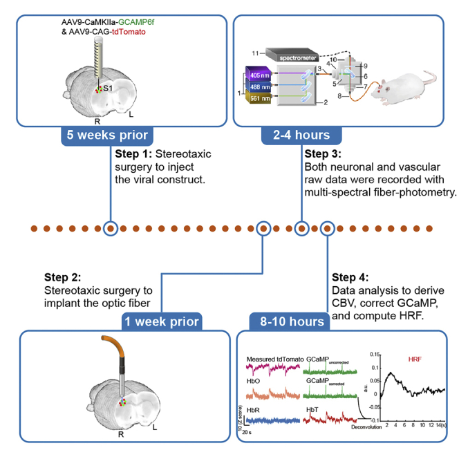
Graphical abstract

Highlights

• •A spectral fiber photometry platform for multi-sensor recordings in the rodent brain
• •Measurement of hemoglobin concentration and blood volume changes
• •Correction of hemoglobin contamination on fluorescent sensor signal
• •Computation of empirical hemodynamic response function

Publisher’s note: Undertaking any experimental protocol requires adherence to local institutional guidelines for laboratory safety and ethics.

Coupling of hemodynamic responses to neuronal activity is the foundation of several functional neuroimaging techniques. Here, we provide three fiber-photometry approaches to simultaneously measure neuronal and vascular signals in the rodent brain using a spectrometer-based system. Two out of these three approaches allow the removal of hemoglobin (Hb)-absorption artifacts and restore the underlying neuronal activity. This technique is applicable to different fluorescent sensors and provides a more accurate measurement of hemodynamic response function in any location of the rodent brain.

Before you begin

The proposed three techniques utilize a spectrometer-based fiber-photometry system (Meng et al., 2018). For labs using non-spectrometer-based photodetectors (Gunaydin et al., 2014; Kim et al., 2016; Lazarjan et al., 2021), this protocol could be adopted by using multiple photodetectors with different bandpass filters (Zhang et al., 2022). The protocol described below focuses on the measurement of neuronal and vascular activity changes simultaneously. We use rats as the representative animal model, but the method is applicable to mouse (data not shown). We introduce the three techniques as follows: (1) The main technique uses GCaMP and tdTomato as the representative reporters in this protocol but is applicable to other reporters. Signals from tdTomato, an activity-independent reporter, are used to derive Hb concentration changes. (2) Optional A uses an excitation paradigm interleaved between 405 nm and 488 nm to obtain activity-independent GCaMP signals. (3) Optional B uses an intravascular fluorescent dye to obtain cerebral blood volume (CBV) changes. For (1) and (2), we leverage the derived Hb concentration dynamics and provide a step-by-step instruction to correct Hb-absorption artifacts in fiber-photometry.

Institutional permissions

All procedures were performed in accordance with the National Institutes of Health Guidelines for Animal Research (Guide for the Care and Use of Laboratory Animals) and approved by the University of North Carolina (UNC) Institutional Animal Care and Use Committee. Readers will need to acquire permission from their relevant institutions.

Setting up the multispectral fiber-photometry system

Timing: Any time prior to the recording

• 1.Assemble and connect all parts of the hardware as shown in Figure 1.
• 2.Install the software to drive the laser and spectrometer.

Figure 1.

Schematic illustration of the photometry system used for measuring green and red fluorescent sensors

The optical components in this four-channel fiber photometry system consist of (1) 405, 488 nm, and 561 nm fiber-coupled laser sources, (2) a compact dichroic mirror set for merging the selected combination of lasers, and (3) a 200 μm core multi-mode optical fiber patch cable connected to the following: a 30 mm cage cubes for fluorescence filter sets with (4) a side fiber port, (5) a neutral density filter, (6) a dichroic mirror, (7) a front fiber port connected to (8) a 200 μm core multi-mode optical fiber patch cable with Ø1.25 mm Ferrule at the distal end, and (9) an emission filter and (10) rear fiber port connected to (11) a 200 μm core multi-mode armored optical fiber patch cable, interfacing with (12) a spectrometer. The 488 nm laser was used for GCaMP and tdTomato excitation. We used the 561 nm laser for Rhodamine B excitation or used interleaved 405 nm laser for GCaMP excitation, which provides GCaMP signals independent of neuronal activity, thus allowing concurrent measurement of Hb-absorption over time.

Stereotaxic surgery to inject viral constructs

Timing: 2 h, 5 weeks prior to the recording

• 3.Prepare the aliquots of viral constructs. Mix GCaMP6f and tdTomato at the volume ratio of 5:1 to make the cocktail for the injection.

CRITICAL: The optimal ratio of GCaMP6f:tdTomato vectors should allow the targeted brain region to emit a similar number of photons excited by the 488 nm laser (Figure 2). The optimal ratio varies depending on the animal genotypes, viral vectors being used, and brain regions.

• 4.Optional A and B: Use GCaMP6f only.
• 5.Anesthetize the rat initially with 5% isoflurane and maintain the anesthetization with a constant flow of 2%–3% isoflurane mixed with medical air.
• 6.Head-fix the rat to a stereotactic frame.
• 7.Open the skin to expose the skull surface and prepare burr holes according to the experimental coordinates.
• 8.Inject 1 μL viral constructs in the primary sensory cortex (S1: AP = +0.5 mm, ML = +3.7 mm, and DV = 1.3 mm) at a flow rate of 0.1 μL/min, as confirmed in Figure 3. Adjust the volume and rate according to the targeted brain region and the experimental animal species being studied.

CRITICAL: After the injection, the micro syringe needle should stay unmoved for 10 min for virus diffusion. Then retract the needle slowly at the rate of 2 mm/min or slower.

• 9.Seal burr holes with bone wax.
• 10.Suture the wound.
• 11.Apply lidocaine jelly around the wound. Give meloxicam orally to further reduce the pain.

Pause point: Allow the research animal 4 weeks for recovery from surgical procedures and virus expression.

Figure 2.

Examples of in vivo spectral signals

The example of GCaMP and tdTomato peaks resulting from the optimal (left) and non-optimal (right) virus ratio used during the injection of the virus cocktail.

Figure 3.

Confocal images confirming the expression of GCaMP and tdTomato

On the left is the low-resolution confocal image of a representative hemisphere of the rat brain. The dashed line highlights the contour of the brain. On the right are the high-resolution images of the brain area with fluorescence signals showing GCaMP alone (top), tdTomato alone (middle), and merged images (bottom). Image is reprinted with permission from (Zhang et al., 2022).

Stereotaxic surgery to implant optic fibers

Timing: 2 h, 1 week prior to the recording

• 12.Cleave the optic fiber to the desired length.
• 13.Repeat steps 5–7.
• 14.Anchor four miniature brass screws to the skull.
• 15.Implant the optic fiber 0.5 mm above the virus injection depth (AP = +0.5 mm, ML = +3.7 mm, and DV = 0.8 mm).
• 16.Seal the implanted components and skull surface with dental cement.
• 17.Repeat steps 10 and 11.

Pause point: Allow the research animal at least 1 week for recovery from surgical procedures before any further experiments.

Install MATLAB and R packages

• 18.Download MATLAB from: https://matlab.mathworks.com/. License is required.
• 19.Download R package from: https://www.r-project.org/. No license is required. R will be called in some MATLAB codes and runs in the background. No need to open R before launching MATLAB.

Key resources table

REAGENT or RESOURCE	SOURCE	IDENTIFIER
Recombinant DNA
AAV9-CaMKIIα-GCaMP6f-WPRE-SV40	U.Penn Vector Core	AV-9-PV3435
AAV9-CAG-tdTomato	UNC Vector Core	N/A
Chemicals, peptides, and recombinant proteins
Rhodamine B, 70,000 MW, Neutral	Fisher Scientific	D1841
Phosphate Buffered Saline (10 ×)	Sigma-Aldrich	P4417
Lidocaine HCl jelly (2%, 5 mL)	UNC SSC Pharmacy	N/A
Meloxicam oral suspension	Henry Schein	N/A
Experimental models: Organisms/strains
Rats: Sprague Dawley (Males, > 8 weeks)	Charles River Laboratories	N/A
Deposited data
Correction for Hb-absorption artifact in fiber-photometry	In this paper	https://doi.org/10.5281/zenodo.6599234
Computation of hemodynamic response function	Chao et al., 2022	https://doi.org/10.5281/zenodo.6599442
Software and algorithms
MATLAB	MathWorks	R2019b; https://matlab.mathworks.com/
RStudio	RStudio Inc.	Version 1.0.136; https://www.r-project.org/
OceanView	Ocean Insight	Version 1.5
Other
Laser combiner	Coherent	Galaxy 8 Laser Combiner, Single Fiber Output, 405, 458, 488, 514, 532, 561, 594, 640 nm
Laser remote	Coherent	OBIS LX/LS Laser Box (50 Ω), 5 Bay with Power Supply and USA Power Cord
405 nm laser∗	Coherent	OBIS LX 405 nm 100 mW Laser, Fiber Pigtail, UFC, Galaxy
488 nm laser	Coherent	OBIS LX 488 nm 100 mW Laser, Fiber Pigtail, UFC, Galaxy
561 nm laser∗∗	Coherent	OBIS LS 561 nm 80 mW Laser, Fiber Pigtail, UFC, Galaxy
Spectrometer	Ocean Insight	QEPRO-FL
Dual-edge dichroic mirror	Chroma	ZT488/561rpc
Dual-band emission filter	Chroma	ZET488/561m
Quad-edge dichroic mirror∗	Chroma	ZT405/488/561/640rpcv2-UF1 25.5 × 36 × 1 mm
Quad-band emission filter∗	Chroma	ZET405/488/561/640mv2 25 mm diameter mounted
4-Bolt HeNe laser to fiber port adapter	Thorlabs	HCL
External C-mount to SM1 thread adapter	Thorlabs	SM1A39
SM1 filter cube	Thorlabs	DFM1
Fiber bundle, 4 fan-out	Thorlabs	BF42LS01
Achromatic fiber port, FC/PC & FC/APC	Thorlabs	PAF2-A4A
Fiber port, SMA	Thorlabs	PAF2S-11A
End cap external threads	Thorlabs	SM1CP2
ND filters, Ø1/2″	Thorlabs	NEK02
SM05 to narrow key FC/APC fiber adapter	Thorlabs	SM05FCA2
SMA fiber adapter for PM20 series	Thorlabs	PM20-SMA
Optic patch cable	Thorlabs	FT200EMT (200 mm, 0.39 NA)
Uncleaved fiber optic cannula	Thorlabs	CFMC12U-20 (200 mm, 0.39 NA)
Smart control panel	Med Associates Inc.	DIG-716P2
Neuro Syringe (2 μL, Gauge = 30)	Hamilton	65459-01
Stereotaxic frame	NeuroStar	N/A

∗For optional A.

∗∗For optional B.

Materials and equipment

Rhodamine B solution

Reagent	Final concentration	Amount
Rhodamine B (powder)	25 mg/mL	25 mg
PBS (10 ×)	n/a	1 mL
Total	n/a	1 mL

Store the solution in fridge (+4°C) and protect from light for a maximum of 3 days.

Step-by-step method details

Fiber-photometry recording

Timing: 2–4 h

For manuals of operating the Ocean QE-Pro spectrometer and its software OceanView, please refer to: https://www.oceaninsight.com/globalassets/catalog-blocks-and-images/manuals--instruction-old-logo/software/oceanviewio.pdf.

• 1.Conduct the experiments either in a dark room or place the animal in a dark chamber.

CRITICAL: To minimize the potential impact of the ambient light, recordings should be performed in a dark environment.

• 2.
  Measure the power of the 488 nm laser at the tip of the patch cable.

  • a.
    Adjust the laser power to get the peak photon count > 1000 (Figure 2) for both GCaMP6f and tdTomato, which empirically yields reliable results.
  • b.
    Usually, set the laser power at ∼ 50 μW and should not exceed 100 μW.

CRITICAL: The 488 nm laser serves as the single laser source for both GCaMP and tdTomato because the brightness of tdTomato (95.22) is more than twice that of GCaMP (43.75, in the presence of Ca²⁺). tdTomato excited by the green laser (e.g., 561 nm) would have been too strong to balance well with the signal from GCaMP. If a different red sensor was used and requires green laser, interleaved recording (Optional A, see below) is recommended as mixed laser source would affect the computation of hemodynamic changes.

• 3.
  Subtract the background noise before connecting the patch cable to the implanted fiber probe.

  • a.
    Click the “light bulb” button while pointing the end of the patch cable to an optical beam trap.
  • b.
    After clicking the “light bulb” button, the background spectrum will be stored and automatically subtracted from subsequently recorded signals.

CRITICAL: If a beam trap is not available, a dark enclosure will suffice as long as there is no reflective surface in the vicinity (20 cm) of the free end of the cable.

• 4.Connect the patch cable with the implanted fiber.
• 5.Start recording.

Note: Problem 1: spectral peaks of GCaMP and tdTomato are unbalanced. See troubleshooting 1.

Note: Problem 2: Noisy data. See troubleshooting 2.

• 6.
  Optional A: Interleaved recording of GCaMP signals with 405 nm and 488 nm excitation lasers.

  Note: This step is an option for multiplexed studies where the red channel is occupied by a functional fluorescent signal (e.g., jRGECO). A spectrometer is highly recommended for this option.

  • a.
    Prepare for the interleaved recording (Figure 4). A master “clock” (e.g., smart control panel, Med Associates Inc., DIG-716P2) is used to control the timing of two lasers and the spectrometer.

    Note: Require dichroic mirror and emission filters for 405 and 488 nm lasers in this setting (see ∗ in key resources table).

  • b.
    Measure the power of 488 nm and 405 nm lasers at the tip of the patch cable.

    • i.
      Adjust the 488 nm laser power to get the peak photon count > 1000 for GCaMP₄₈₈. The required power is usually ∼ 50 μW,
    • ii.
      405 nm laser usually requires a higher power due to the much weaker GCaMP₄₀₅ emission signal.
  • c.
    Record the background noise signals with the interleaved paradigm for 2 min (for details on how to record the background noise, please see Main step 3).

    Note: Background noise is not automatically subtracted in this option. The mean of the background noise will be subtracted manually in the data processing.

  • d.
    Connect the patch cable with the implanted fiber.
  • e.
    Start interleaved recording.

    Note: Problem 3: frame loss during interleaved recording. See troubleshooting 3.

• 7.
  Optional B: Intravenous injection of Rhodamine B to obtain CBV signals.

  Note: For groups equipped with a spectrally resolved spectrometer, this option is suboptimal. For groups equipped with non-spectrally resolved photodetectors, adding an extra red channel to measure the Rhodamine B in addition to the green channel of the GCaMP signal is a robust approach to measure neuronal and vascular activity simultaneously.

  • a.
    Dissolve Rhodamine B (Fisher Scientific, 25 mg) powder with 1 mL sterile PBS (0.1 M).
  • b.
    Inject the Rhodamine B via tail vein at the dose of 25 mg/kg.

    Pause point: Wait for at least 30 min for the Rhodamine B signal to get stabilized.

    CRITICAL: A 30-min wait is necessary because, following the injection of Rhodamine B bolus, the signal follows a fast exponential decay and then stabilizes in about 30 min.

  • c.
    Measure the power of 488 nm and 561 nm lasers at the tip of the patch cable.

    • i.
      Adjust the laser power to get the peak photon count > 1000 for both GCaMP6f and Rhodamine B (Figure 5).
    • ii.
      Usually, set the laser power at ∼ 50 μW and should not exceed 100 μW.
  • d.
    Subtract the background noise.
  • e.
    Connect the patch cable with the implanted fiber.
  • f.
    Start recording.

Figure 4.

Interleaved acquisition paradigm with 405 nm and 488 nm excitation lasers

Ca²⁺-independent GCaMP signals (GCaMP₄₀₅) were excited by a 405 nm laser, whereas Ca²⁺-dependent GCaMP signals (GCaMP₄₈₈) were excited by a 488 nm laser. This interleaved paradigm was used because GCaMP₄₀₅ and GCaMP₄₈₈ share nearly identical emission spectra and thus cannot be spectrally unmixed. Data were acquired at 50% duty cycle every 50 ms using a box-paradigm to avoid spectrometer frame loss during the trigger mode. The final sampling rate is 10 Hz for all signals. Images are reprinted with permission from (Zhang et al., 2022).

Figure 5.

An example of in vivo spectral signals of GCaMP6f and Rhodamine B

Preprocessing

Timing: 10 min

Full emission spectra of GCaMP, Rhodamine, and tdTomato could be downloaded from https://www.chroma.com/spectra-viewer.

MATLAB codes to generate the reference spectra of GCaMP, Rhodamine, and tdTomato are available here: https://github.com/CAMRIatUNC/MakeReference.

• 8.Generate the reference emission spectra for measured signals. This step only needs to be run once for each fluorophore.

[ref1]= make_reference(em_txt_file1,wavelength,emiss_filter_index)

[ref2]= make_reference(em_txt_file2,wavelength,emiss_filter_index)

ref=[ref1,ref2];

CRITICAL: Compare the generated reference emission spectra carefully with the real data. There might be a systematic error which is related to each spectrometer. We recommend generating the reference emission spectra for each spectrometer.

Linear unmixing, deriving the vascular changes, and correction of Hb-absorption

Timing: 30 min

MATLAB codes for hemodynamic correction are available here: https://github.com/CAMRIatUNC/HemoCorrection.

• 9.Compute the uncorrected GCaMP, uncorrected tdTomato, oxygenated Hb (HbO), deoxygenated Hb (HbR), and total Hb (HbT) as follows:

Note: Run the script in the same directory where the raw text file generated by the spectrometer was saved.

tmp = detectImportOptions(TextFile);%TextFile is the raw data file

NumOfHeaderlines = tmp.DataLines(1,1);

M = dlmread(TextFile,'\t',NumOfHeaderLines,2);

M = M';

[Output]=HemoCalcGreen163(M);

Note: Problem 4: empirically, the goodness-of-fit (L) ≤ 0.05 is considered acceptable for fitting the hemodynamic changes. For goodness-of-fit (L) > 0.05, see troubleshooting 4.

• 10.Optional A: For the interleaved recording of GCaMP signals with 405 nm and 488 nm excitation lasers, compute the HbO, HbR, HbT, GCaMP₄₈₈, and GCaMP₄₀₅ as follows:

Note: Run the script in the same directory where the raw text file generated by the spectrometer was saved.

[BG488,BG405]=interleaving_fix_V2(BG_file,’datalength’,1200,’hz’,10,’interp’,’no’); % BG_file: Background raw text file

[G488,G405]=interleaving_fix_V2(DATA_file,’datalength’,7920,’hz’,10,’interp’,’yes’);% DATA_file: Real raw data file

mean_BG405 = nanmean(BG405,2); mean_BG488 = nanmean(BG488(:,2:end),2);

% Next manually subtract the background noise and discard the first 6-min data

G405_fix = G405 – mean_BG405; G405_fix = G405_fix(:,4801:end);

G488_fix = G488 – mean_BG488; G488_fix = G488_fix(:,4801:end);

G488_uncor = sum(G488_fix(200:230,:),1)’;

G405_uncor = sum(G405_fix(200:230,:),1)’;

[Output] = HemoCalcBlue400(G405_fix);

• 11.
  Optional B: For GCaMP and Rhodamine B data, perform linear unmixing and compute ΔF/F of GCaMP and Rhodamine B for changes in neuronal and vascular signal, respectively.

  • a.
    Linear Unmixing.

    tmp = detectImportOptions(TextFile);%TextFile is the raw data file

    NumOfHeaderlines = tmp.DataLines(1,1);

    M =dlmread(‘RhodamineSampleData.txt’,'\t',NumOfHeaderLines,2);

    ref= csvread(‘Dual-GCaMP&Rho.csv’,1,1);

    coef=zeros(size(ref,2),size(M,1));

    for i=1:size(M,1)

     coef(:,i)=lsqnonneg(ref(140:500,:),M(i,140:500)');

    end

    coef = coef’;
  • b.
    Compute ΔF/F, then skip step 12.

    deltaCoef1 = (coef(:,1) – mean(coef(1:290,1))) ./std(coef(1:290,1));

    deltaCoef2 = (coef(:,2) – mean(coef(1:290,2))) ./std(coef(1:290,2));

    % 290 is the length of the baseline.

    Note: Problem 5: empirically, the goodness-of-fit R² ≥ 0.90 is considered acceptable for the linear unmixing. For R² < 0.90, see troubleshooting 5.

• 12.Correction of Hb-absorption artifacts in GCaMP and tdTomato signals.

[G_cor,G_uncor_perc]=BlueSignalsCorrectedbyHb(G_uncor,HbO,HbR);

[Td_cor,Td_uncor_perc]=GreenSignalsCorrectedbyHb(Td_uncor,HbO,HbR);

Computing the hemodynamic response function (HRF)

After deriving vascular activity changes and corrected GCaMP signal dynamics, HRF can be calculated via deconvolving the vascular activity time-course with the concurrently measured GCaMP time-course. Detail methods can be found in (Chao et al., 2022). We use a homemade script running in MATLAB for the HRF calculation, which is available at https://github.com/CAMRIatUNC/Photometry-tools/blob/main/HRF.m.

• 13.Make sure the HRF.m is located under your MATLAB folder or under one of your Set Path folders.
• 14.Import the vascular and GCaMP activity time-courses into MATLAB as single column variables.
• 15.Once the vascular and GCaMP activity time-courses were imported, HRF could be calculated as follows:

Sampling_rate = 10; % in Hz;

HRF_length = 25; % in seconds;

[hrf]=HRF(GCaMP time-course, Vascular time-course, Sampling_rate, HRF_length);

Note: Problem 6: noise and baseline drift in neuronal and vascular time-courses. See troubleshooting 6.

Expected outcomes

In contrast to studies using non-spectrally resolved fiber-photometry, the strategy proposed in this protocol expands the scope of fiber-photometry by generating “free-of-charge” hemodynamic signals from control fluorescent sensors (e.g., tdTomato). Changes in HbO and HbR (ΔHbO and ΔHbR) could be derived from measured tdTomato signals (Figure 6, left). ΔHbO and ΔHbR were also used to correct for the Hb-absorption artifacts in the measured GCaMP signals (Figure 6, middle). The amount of ΔHbO and ΔHbR brings about changes in HbT (ΔHbT), which informs CBV changes. Lastly, HRF was estimated by deconvolution of HbT changes to corrected GCaMP changes (Figure 6, right). Similarly, the results of Optional A are shown in Figure 7A, with a lower contrast-to-noise ratio (CNR) in hemodynamic changes due to the weak emission signal of the GCaMP excited by the 405 nm laser (Zhang et al., 2022). The expected results of Optional B are shown in Figure 7B. No correction of GCaMP signals was performed because ΔHbO and ΔHbR are not accessible in this method.

Figure 6.

Expected results of changes in neuronal and vascular activity and derived HRF

This representative dataset was generated from a single session with three triggered stimuli. HRF was calculated by deconvoluting HbT changes (derived from measured tdTomato signals) and Hb-absorption-corrected GCaMP signals.

Figure 7.

Expected results of Optional A and B demonstrating changes in neuronal and vascular activity

Gray-shaded segments in (A) and (B) indicate the stimulation period.

Limitations

Lack of access to ground-truth GCaMP signals remains an obstacle to unequivocally validate the “corrected” GCaMP generated in this protocol (Zhang et al., 2022). In addition, the linear unmixing of two signals and the calculation of hemodynamic parameters are highly dependent on the quality of the spectral data. Any factors that affect the quality of the spectrometer data may cause unsuccessful unmixing or fitting. For the quality control of the spectral data, please refer to Problems 1, 2, 4, and 5.

Troubleshooting

Problem 1

Unbalanced peaks in step 5.

For the best results, the signal intensity of different peaks acquired from the spectrometer would be ideal to be within a similar range. An extremely unbalanced signal (Figure 2) would result in inaccurate linear unmixing and fitting.

Potential solution 1

Adjust the ratio of GCaMP:tdTomato in the cocktail viral mixture.

Potential solution 2

Adjust the output power of laser beams if different lasers were used to excite different fluorophores.

Problem 2

Noisy spectral data in step 5.

For the best signal-to-noise ratio, the photon count of each peak should be over 1000 and the spectral shape of each component should fit their reference spectra well. Spectra data with too much noise may result in inaccurate linear unmixing and fitting.

Potential solution 1

Disconnect the patch cable and reconnect it to the implanted fiber to make sure the connection is tight.

Potential solution 2

If the fiber is tangled, detangle it.

Potential solution 3

Increase the laser power, but not exceeding 100 μW. Keep in mind that the background subtraction needs to be performed again every time the laser power was adjusted.

Potential solution 4

Re-do the background subtraction.

Problem 3

Frame loss in step 6e.

For interleaved recording with the trigger mode in OceanView, frame loss may occur.

Potential solution 1

Adjust the ‘integration time’ in OceanView. Frame loss is due to an insufficient gap between consecutive recording windows. This gap is essential for handling the rapidly triggered recording mode. We recommend reducing the integration time. For example, setting it to 25 ms (50% duty cycle) for the 50 ms box-paradigm (see Figure 4) can avoid frame loss.

Potential solution 2

Precious experimental data with frame loss could be salvaged by setting the ‘interp’ to ‘yes’ in steps 10 Optional A.

Problem 5

Unsuccessful fitting of linear unmixing (R² < 0.9) in step 11b.

During the linear unmixing to separate two components (e.g., GCaMP and tdTomato or Rhodamine B), the goodness-of-fit (R²) may be below 0.9, suggesting suboptimal fitting.

Potential solution 1

Make sure that the peaks of reference spectra match well the peaks of the experimental data.

Potential solution 2

Exclude the data points that contain the noise. The default fitting range is 450–750 nm, which could be edited in the MATLAB script.

Problem 6

Noise and signal drifting problem in step 15.

For the best results, neuronal and vascular signals may need to be de-noised or de-trend before further analysis (e.g., HRF computation). Here we provide example filters that are commonly applied to de-noise and de-trend.

Neuro = filter_2sIIR(GCaMP_vector',[0.01],10,5,'high')';

Vascular = filter_2sIIR(CBV_vector',[0.01 0.3],10,5,'bandpass')';

Potential solution 1

Various types of filters can be applied. Justify scientifically and adjust the filter setting to meet specific research goals.

Potential solution 2

Discard the segment of data that shows significant drift or noise.

Resource availability

Lead contact

Further information and requests for resources should be directed to and will be fulfilled by the lead contact, Wei-Ting Zhang (wtzhang@email.unc.edu).

Materials availability

This study did not generate new unique reagents.

Data and code availability

The protocol includes all datasets analyzed during this study. Sample data and codes: https://doi.org/10.5281/zenodo.6599234. Codes for HRF calculation: https://doi.org/10.5281/zenodo.6599442.

References

- Chao T.-H.H., Zhang W.-T., Hsu L.-M., Cerri D.H., Wang T.W.W., Shih Y.-Y.I. Computing hemodynamic response functions from concurrent spectral fiber-photometry and fMRI data. Neurophotonics. 2022;9:032205. doi: 10.1117/1.nph.9.3.032205. [DOI] [PMC free article] [PubMed] [Google Scholar]
- Gunaydin L.A., Grosenick L., Finkelstein J.C., Kauvar I.V., Fenno L.E., Adhikari A., Lammel S., Mirzabekov J.J., Airan R.D., Zalocusky K.A., et al. Natural neural projection dynamics underlying social behavior. Cell. 2014;157:1535–1551. doi: 10.1016/j.cell.2014.05.017. [DOI] [PMC free article] [PubMed] [Google Scholar]
- Kim C.K., Yang S.J., Pichamoorthy N., Young N.P., Kauvar I., Jennings J.H., Lerner T.N., Berndt A., Lee S.Y., Ramakrishnan C., et al. Simultaneous fast measurement of circuit dynamics at multiple sites across the mammalian brain. Nat. Methods. 2016;13:325–328. doi: 10.1038/nmeth.3770. [DOI] [PMC free article] [PubMed] [Google Scholar]
- Lazarjan V.K., Gashti A.B., Feshki M., Garnier A., Gosselin B. Miniature fiber-spectrophotometer for real-time biomarkers detection. IEEE Sens. J. 2021;21:14822–14837. doi: 10.1109/JSEN.2021.3072578. [DOI] [Google Scholar]
- Meng C., Zhou J., Papaneri A., Peddada T., Xu K., Cui G. Spectrally resolved fiber photometry for multi-component analysis of brain circuits. Neuron. 2018;98:707–717.e4. doi: 10.1016/j.neuron.2018.04.012. [DOI] [PMC free article] [PubMed] [Google Scholar]
- Zhang W.-T., Chao T.-H.H., Yang Y., Wang T.-W., Lee S.-H., Oyarzabal E.A., Zhou J., Nonneman R., Pegard N.C., Zhu H., et al. Spectral fiber-photometry derives hemoglobin concentration changes for accurate measurement of fluorescent sensor activity. Cell Rep. Methods. 2022 doi: 10.1016/j.crmeth.2022.100243. [DOI] [PMC free article] [PubMed] [Google Scholar]
Associated Data
This section collects any data citations, data availability statements, or supplementary materials included in this article.
Data Availability Statement