What lowered inflation in India: monetary policy or commodity prices?

Abstract

India has seen lower inflation by historical standards for the past 6 years. This has been attributed to the adoption of inflation targeting by the central bank, the Reserve Bank of India in 2016. In particular, it has been asserted that the lower inflation reflects the anchoring of expectations. We evaluate these claims. An econometric investigation indicates that there is no basis to the claim that inflation has been lowered due to the anchoring of expectations. On the other hand, we are able to account for the trajectory of inflation in India after 2016 in terms of an alternative explanation of inflation, namely the structuralist.

Introduction

In 2015, India’s parliament amended the Reserve Bank of India (RBI) Act of 1933 to make inflation control the sole objective of monetary policy. The amendment mandated RBI to pursue an inflation target of 4%, measured in terms of the Consumer Price Index (CPI), with a tolerance band of ± 2 percentage point. This arrangement came into effect from August 5, 2016 and was to last till March 31, 2021. With it, the RBI made the transition to an inflation targeting (IT) central bank. In the 5 years, inflation has mostly remained within the target range. As per the original terms of agreement between the India’s government and its central bank, the policy of inflation targeting was reviewed after 5 years and the original mandate was renewed. Prior to the official verdict, academic evaluations had appeared. These had concluded that inflation targeting in India had succeeded and that this had been achieved by the anchoring of inflation expectations by the RBI.1 We investigate this claim. Our view is that for the claim that inflation targeting has succeeded, it is necessary to first establish that the central bank has actually controlled inflation. This would require demonstrating that the inflation model on which the policy of inflation targeting is based, namely the New Keynesian Phillips Curve (NKPC), with its emphasis on forward-looking expectations is empirically valid in the Indian case. Evaluations claiming the success of inflation targeting in India have not been accompanied by such an exercise. In its absence, there would be no basis for the claim that it is inflation targeting that is responsible for the observed path of inflation in India since 2016. In this paper, we first investigate the claimed effectiveness of inflation targeting in having lowered the inflation rate in India. Next, we provide an explanation of the observed trajectory of inflation after the adoption of inflation targeting.

Background: anti-inflation policy before inflation targeting

Inflation targeting is only one of a set of possible inflation control policies. Thus, skepticism about the efficacy of inflation targeting, which is a particular strategy, does not imply rejection of inflation control as a legitimate objective of economic policy. This is worth emphasizing as it is not well understood. Even before inflation targeting was advanced, Friedman had brought inflation control to the center of macroeconomics through repeated references to the dangers of inflation. As a monetarist, Friedman had prescribed money supply-targeting as the means to control inflation. On the other hand, under inflation targeting, it is the use of the interest rate to target inflation that is prescribed. Therefore, what is new about inflation targeting is only the instrument chosen, not the goal itself.2 There is, however, the implicit suggestion that inflation targeting is more effective than the erstwhile monetarist approach, as the instrument—the policy interest rate—is directly under the control of the central bank, in a way that the money supply is not. However, what has mostly remained hidden in the public discourse is the empirical validity of the economic model that underlies inflation targeting. Given our objective in this paper, it is worth repeating that it cannot simply be assumed that this model is a valid representation of the inflationary process. This must be demonstrated.

Recent inflation in India

To identify the role played by inflation targeting in lowering inflation in India, we start by first studying its recent history. Figure 1 may be seen the trajectory of annual inflation on a quarterly basis from the year 2000 onwards, including the period from the first quarter of the financial year 2016. Details of the sources of data used in this study are given in the Appendix A1 and Appendix A2 presents the results on the unit root properties of the variables used in this study.

Fig. 1.

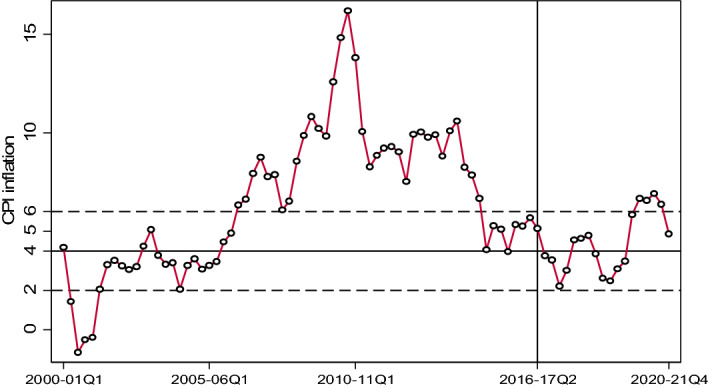
The trajectory of inflation in India

When interpreting the data, it would be useful to bear in mind that inflation targeting was adopted in 2016. Five observations may be made on the basis of this history. First, it can be asserted that inflation has been lowered very significantly in India over the past decade. From a high of 15% in 2009–10 (Q4), inflation hit a low of 4% in 2014–15 (Q3). Second, since 2016, the inflation rate has mostly remained within the prescribed band. Third, it begins to rise about 3 years into the experiment, in September 2019. As this is before the lockdown in response to the COVID-19 pandemic, the increase cannot be put down to an extraordinary event. Fourthly, even if it is said that inflation has remained within the band for much of the time since inflation targeting was adopted, it had entered the prescribed band some 7 quarters before 2016, having been on a downward trend for at least a year before entering the band. This should alert us to the possibility that factors other than inflation targeting may have been responsible for lowering inflation in India. At least, it would be premature to claim a role for inflation targeting without investigating the matter. Finally, inflation has remained within the band of 4 ± 2%, and for a longer period, even in the distant past, in the early 2000s, once again suggesting a role for other factors in its determination.

In a preliminary attempt to understand the determinants of inflation, we study movements in the principal components of the consumer price index. From the data in Table 1, we can see a steady decline in food-price inflation since 2012–13. In fact, this decline is greater than the decline in the inflation rate, implying a decline in the relative price of food. It gives reason to believe that declining food-price inflation has had a role in the decline in inflation. The behavior of ‘core’ inflation, or inflation excluding food and fuel price movements, also declining in this period, though not as sharply, suggests that it may not be autonomous of the behavior of food prices. In fact, it may have been driven by it. If that is so, the case for targeting core instead of headline inflation, a proposition always on the agenda of international policy entrepreneurs and repeated by India’s government economists, weakens. The data in Table 1 establish that inflation in India was trending downward well before 2016 and had settled into the band, or stabilized, a full 2 years before IT was adopted.

Table 1.

Inflation by components of the consumer price index

	2012–13	2013–14	2014–15	2015–16	2016–17	2017–18	2018–19	2019–20	2020–21
Consumer price index	10.2	9.5	5.8	4.9	4.5	3.6	3.4	4.8	6.2
Food and beverages	11.9	11.1	6.5	5.1	4.4	2.2	0.7	6	7.3
Core inflation	8.7	8.1	5.4	4.6	4.8	4.6	5.8	4	5.5

Source: Reserve Bank of India; https://www.rbi.org

Can anchored expectations describe recent inflation in India?

It is asserted that inflation targeting works via the anchoring of inflation expectations by the central bank. Accordingly, it has been claimed that inflation in India has been contained within the target range since 2016 because the RBI successfully anchored the expectation of inflation.3 We now investigate the claim. Figure 2 presents 3-month ahead and 1-year ahead inflation expectations of households and actual inflation. The inflation expectation data are from the households’ inflation expectations surveys conducted periodically by the RBI. The expected inflation rates are averages across households. Visual inspection of the graphs suggests the following. First, for the period from 2016—when inflation targeting was adopted—while there is slight upward movement in the 3-month ahead inflation expectations, and none for 1-year ahead inflation expectations, actual inflation has a distinctly cyclical trajectory. Second, while expectations have been relatively steady since 2016, suggesting that they have been anchored, they had been revised downwards dramatically in the 2 years prior to that, when inflation targeting had not yet been adopted. Third, even if it were to be asserted that expectations have been anchored after 2016 they have remained higher than the upper end of the target range and at times far higher than the target itself.4 Finally, actual inflation has fluctuated considerably more than expectations, implying that the latter are unlikely to have been a major factor in driving inflation. These facts make it difficult to sustain the argument that inflation in India has been tamed by anchoring expectations.

Fig. 2.

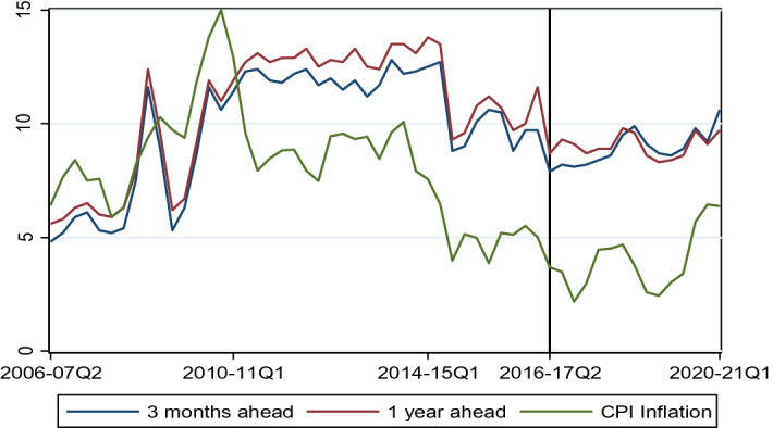
Households’ inflation expectations and actual inflation

We now investigate econometrically the role of inflation expectations in the dynamics of inflation in India using the “canonical form”5 of the NKPC,

$$\mathrm{\Delta }{p}_t={\beta E}_t{\mathrm{\Delta }p}_{t+1}+c_0+{\gamma y}_t$$ 1

where ∆p_t stands for the inflation rate, E_t∆p_t+1 is the expectation at time t of inflation in the next period, y_t is the output gap, and β and ϒ are positive constants.

Note that in this specification, expectations are forward-looking. Thus, there is no ‘intrinsic’ inertia to inflation. However, motivated by the discovery of inertia in practice, Gali & Gertler, (1999) recommend augmentation of the NKPC by including the one period lagged inflation rate. Inclusion of lagged inflation along with forward inflation rate implies that sub-set of firms is using “a backward-looking rule of thumb to set prices”.

The resulting model, specified as follows:

$$\mathrm{\Delta }{p}_t={{\beta }^{a}E}_t{\mathrm{\Delta }p}_{t+1}+{{{\beta }^b\mathrm{\Delta }p}_{t-1}+c}_0+{\gamma x}_t$$ 2

is termed by them “the hybrid New Keynesian Phillips Curve”.6 We find this classification of firms into two categories according to their expectation formation mechanism to be ad hoc. However, as it is often found in the literature, we use this very specification so that our estimates are comparable.

Two considerations arise when estimating Eq. (1). First, we need a measure of the output gap. We follow the standard practice of using the Hodrick–Prescott (H–P) filter to estimate the trend and treat the deviation of log of actual output from its trend value for each year as the output gap. However, as the H–P filter has been subjected to criticism, we also use a second measure of the output gap, identified as D–T, which is the deviation of output from a polynomial trend with quarterly dummies.7 Here, the underlying assumption is that the natural level of output evolves along a trend, and deviations from it are considered as the cycle.8 Second, we would need data on expectations, which are unobservable. For this variable, we use survey data on expected inflation of households released by the RBI. The model was estimated by OLS and GMM-IV alternately. In the GMM-IV estimation, the output gap and expected inflation were treated as endogenous, and, therefore, instrumented. Instruments are the lagged values of the output gap selected on the basis of its correlation with the current value of the output gap. The results are presented in Table 2. In the Table, columns numbered (1) and (2) report the OLS estimates and columns (3) and (4) report GMM-IV estimates. Note that the estimated coefficients of expectations are not statistically significant.9 The measures of output gap are significant in two cases, though with a negative sign, thus contradicting the theory underlying the NKPC.

Table 2.

Estimates of the NKPC with survey-based expectations

	(1)	(2)	(3)	(4)
One period lagged inflation	0.457**	0.450**	0.463**	0.440**
	(3.57)	(3.49)	(4.24)	(5.92)
Expected inflation (3 months ahead)	0.000228	0.000334	− 0.000922	0.000129
	(0.33)	(0.46)	(− 1.17)	(0.15)
Output gap (HP)	0.0280		− 0.241**
	(0.84)		(− 5.43)
Output gap (D–T)		0.0330		− 0.161**
		(0.96)		(− 4.10)
Oil price (growth rate)	0.0187	0.0168	0.0916**	0.0706**
	(1.05)	(0.94)	(6.81)	(3.79)
q1	0.0204**	0.0182**	0.00697**	0.0208**
	(3.91)	(4.00)	(2.71)	(7.37)
q2	0.0291**	0.0261**	0.0154**	0.0338**
	(6.01)	(5.65)	(5.38)	(11.17)
q3	0.00890*	0.00882*	0.00257	0.00499**
	(2.06)	(2.08)	(1.82)	(3.34)
Constant	− 0.00696	− 0.00660	0.0124	− 0.00626
	(− 1.06)	(− 1.08)	(1.76)	(− 0.83)
Observations	55	55	46	46
Adjusted R2	0.533	0.535	0.067	0.264
Hansen’s J (χ2)			1.375	1.573
p value			0.711	0.665

(1) t statistics in parentheses, (2) ** and * indicate significance at the 1 and 5 percent level, respectively, (3) q1 … q3 are quarterly dummies

These estimates of the NKPC for India point conclusively to it being a poor representation of inflation in the country.10 Our finding of the lack of validity of the output gap model for Indian data is in line with the findings of other researchers, see Paul (2009) and Hatekar, Sharma and Kulkarni (2011). Before it may be assumed that this finding reflects some developing-economy pathology, it may be noted that the output gap model is not always validated for the United States economy either.11 Our finding of the insignificance of inflation expectations when the NKPC is estimated for India is consistent with the argument of Rudd, (2021) that the theoretical basis for the role of expectations in inflation is weak. That is, it has simply been assumed.

We have used headline inflation as our measure. The output gap model has been validated for India using core inflation as the measure (see: Ball and Mishra, 2016). Two comments would be in order here. First, India’s central bank targets headline inflation, so it is headline inflation that needs to be addressed when evaluating the record of IT in the country. Second, in a separate investigation, we have found that core inflation is related to agricultural-price inflation which is part of headline inflation. This association has two implications. First, core inflation has no autonomous status. Second, the RBI cannot control core inflation without first stabilizing agricultural-price inflation.

Does the finding that the NKPC is without statistical validity when confronted with Indian data leave us without an explanation of inflation in the country? We now turn to this issue.

Commodity price movements and recent inflation in India

An explanation of inflation other than that implied by the New Keynesian Phillips Curve has actually existed for far longer. Though developed several decades prior to the emergence of inflation targeting, it did not receive attention in the mainstream, because the framework within which it was embedded was developed for the analysis of the developing economies.12 Specifically, this explanation of inflation was originally meant for Latin America’s economies, but it has applicability for much of the developing world, especially India. This structuralist model of inflation is a sub-set of a larger model of the economy that can explain both output and inflation. Crucially, it generates outcomes that are observed in India which cannot be explained by the Phillips Curve. These are disinflationary expansions and inflationary recessions. They stem from the presence of an agricultural sector, with characteristics different from that of industry, as demonstrated by Balakrishnan and Parameswaran (2021).

In structuralist macroeconomics, the economy is modeled as consisting of two sectors, agriculture and industry, with price and output determination mechanisms varying between the two. The agricultural price clears the market in each period, i.e., it is determined by supply and demand, while the industrial price is cost-determined, with a fixed mark-up. The output of agriculture is considered exogenous, as it is driven by weather, while industrial output is demand-determined. Industrial costs are made up of labor and material costs, notably the price of imported oil. The price of oil is determined in the global market while the wage is related to the general price level, though with a lag. In this model, it is seen13 that inflation (π) is positively related to the relative price of the agricultural good (θ), industrial costs $(\gamma W_t+\tau e{P}_{m,t})$ and lagged inflation as follows14:

$${\pi }_t=[\left(\frac{1}{P_{t-1}}\right)(1+r)\{\alpha {\theta }_t+(1-\alpha )\}(\gamma W_t+\tau e{P}_{m,t})]-1$$ 3

Comparative statics applied to this model show that a rise in the inflation rate can occur from either an expansion of industry or a decline in agricultural output. This feature has the implication that we can make no definite judgment about the level of activity, in particular, whether actual output exceeds the natural level, by observing the change in the inflation rate. Surely, inflation due to a negative agricultural shock cannot reasonably be interpreted as a case of the economy ‘over-heating’ due to output expansion.

Estimates of the structuralist model of inflation for India

We estimated the structuralist inflation model for India using quarterly data and over the same sample period as we had earlier done with the NKPC. The choice of variables in the econometric specification of the structuralist model is based on Eq. (3). The relative price of the agricultural good is the ratio of implicit GDP deflator of Agriculture, Forestry and Fishing to that of non-agriculture sector, which includes Construction, Manufacturing and Services. As the relative price was found to be non-stationary, its log difference (growth rate) was used.15 Allowing for the possibility that relative price is endogenous in the econometric model, the model has been estimated using both OLS and GMM-IV. The instruments used are the lagged values of the growth rate of relative price and growth rate of agricultural GDP. All lags up to ten with absolute value of correlation coefficient of 0.30 or above with the current value of growth rate of relative price are taken as instruments. The results are presented in Table 3. As the OLS and GMM-IV estimates are, mostly, very close to one another we make no distinction between them when discussing the results. First, the coefficient on the relative price of agricultural goods is statistically significant and quite high. As in the theoretical model, the price of oil matters for inflation, though the coefficient is far lower than that for the relative price. Lagged inflation matters for current inflation, implying inertia. Inflation inertia has the implication that inflation cannot be ended merely through central bank announcements termed “communication”. Finally, the explanatory power of the model—seen in the adjusted R²—is quite high for a model in changes. These results justify the conclusion that structuralist inflation model is a valid description of the inflationary process in India, in particular that the relative price of agricultural goods is the principal driver of inflation.

Table 3.

Estimates of the structuralist model of inflation

	(1)	(2)
	OLS	GMM-IV
Relative price (growth rate)	0.306**	0.340**
	(5.74)	(4.29)
Oil price (growth rate)	0.0380**	0.0390**
	(3.40)	(7.32)
Lagged inflation	0.399**	0.446**
	(5.57)	(19.03)
q1	0.0117**	0.0140**
	(3.22)	(6.07)
q2	0.0191**	0.0178**
	(5.19)	(8.05)
q3	0.00646*	0.00647**
	(2.03)	(6.17)
Constant	− 0.00201	− 0.00356**
	(− 0.75)	(− 3.43)
Observations	95	87
Adjusted R2	0.616	0.686
Hansen’s J (χ2)		1.543
p value		0.672

Dependent variable is CPI inflation; period is 1996–97(Q1) to 2020–21(Q1)

(1) t statistics in parentheses

(2) ** and * indicate significance at the 1 and 5% level, respectively

(3) q1 … q3 are quarterly dummies

Interpreting lower inflation in India since 2016

On the basis of the econometric evidence for the two models of inflation in the Indian context, it may be surmised that the stable inflation since the adoption of inflation targeting in 2016 owes to the behavior of the relative price of agricultural goods and the price of imported oil. This is confirmed by the following exercise. We use the OLS estimate of the structuralist inflation model estimated using data upto 2016–17(Q2), to predict inflation after inflation targeting was adopted up to 2020–21 (Q1), being the last year for which data were available when the exercise was conducted. The time series of the actual and predicted inflation rates are graphed in Fig. 3. A close fit may be seen.16 In particular, that the predictions from a structuralist inflation model show a downward trend after 2016, the year in which inflation targeting was adopted. This implies that the observed trajectory of inflation can be fully understood within the framework of structuralist macroeconomics. This combined with our finding that expectations do not drive inflation, and that the output gap in the NKPC is not statistically significant, implies that it would be wrong to attribute this trajectory to the monetary policy of the RBI, in particular inflation targeting.

Fig. 3.

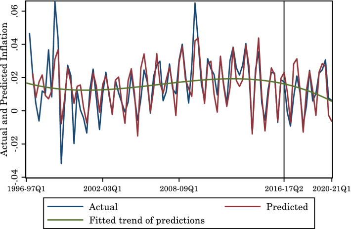
Predictions based on the structuralist model

As the main determining variable of inflation in the structuralist model is the relative price of agricultural goods, we investigated the change in its growth rate for the period under consideration. Rates of growth for sub-periods established by the Bai-Perron (1998) method are presented in Table 4. A statistically significant reduction in the rate of growth of the relative price is evident from 2011 to 12. The reduction is very strong from 2017 to 18 onwards. The results of our econometric investigation, taken together, lend high credence to the conclusion that the lowering of inflation in India since 2011, and particularly since 2016, owes overwhelmingly to the slower growth of commodity prices.

Table 4.

Growth rates of the relative price of agricultural goods

Period	Growth rate (in %)
1996–97 Q1 to 2000–01 Q1	0.00
2000–01 Q2 to 2004–05 Q3	− 0.45
2004–05 Q4 to 2010–11 Q4	0.93
2011–12 Q1 to 2017–18 Q3	0.69
2017–18 Q4 to 2020–21 Q1	0.28

The exponential growth rate is reported. The breakdates have been estimated

Finally, in Fig. 4, is presented a plot of inflation and the growth of the relative price of agricultural goods. A co-movement is evident, with the relative price change leading inflation. The correlation coefficient is 0.59.

Fig. 4.

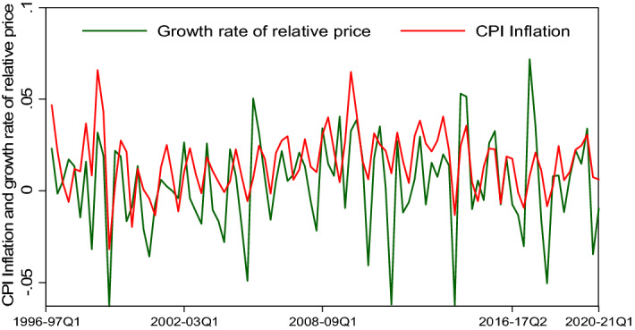
Inflation and the relative price of agricultural goods

Conclusion

In 2021, India completed 5 years of inflation targeting. Reviews have asserted that the fact of inflation remaining within the mandated band is evidence of the success of inflation targeting. We have argued here that such an approach cannot exclude observational equivalence, that observed inflation may have been generated by a process other than the one assumed under inflation targeting, the New Keynesian Phillips Curve. Accordingly, we investigated which of two alternative models of inflation account for the Indian experience. It was found the New Keynesian Phillips curve, on which central banks across the world base inflation targeting, is not validated for Indian data but the structuralist model of inflation, based on the relative price of agricultural goods, is. Further, the latter model was found to predict, upto a considerable degree of accuracy, the trajectory of inflation after inflation targeting was adopted. This implies that subdued inflation in India, observed for almost a decade by now, can be put down to the behavior of commodity prices. Now, control of inflation would require a different set of instruments than what is available to central banks.

Appendix: A1. Data sources

The definition and construction of variables have been explained as and when they appear in the text. Here we state the sources of the data used.

Output: The study used quarterly GDP data for the period 1996–97 Q1 to 2020–21 Q1. The quarterly GDP data in current and constant prices were collected from the website of the Central Statistical Office (CSO).

Prices: Following the RBI, the inflation rate is measured by the rate of change in the consumer price index (CPI). For the years for which a single consumer price index is unavailable a combined index has been formed by combining the CPI for Industrial Workers and the CPI for Agricultural Workers. Oil price has been measured by the wholesale price index for mineral oils. All price data are from the EPW Research Foundation’s ‘India Time Series’ database. The GDP deflators for the agricultural and non-agricultural sectors, used in the construction of the relative price, are computed from data on sectoral GDP at current and constant prices taken from the national accounts statistics.

Inflation Expectations: Expectations data are from the Household’s Inflation Expectations Survey of RBI, available for downloading from the website www.rbi.org.in.

Averages of the expected inflation across households are used in the econometric estimation.

A2. Testing for a unit root and seasonal stability

Unit root properties of the time series were tested using the Augmented Dickey–Fuller (ADF) test, the Kwiatkowski, Phillips, Schmidt, and Shin (KPSS) test, and the Zivot and Andrews test. The Zivot-Andrews test is used because a trend stationary series with a break in the trend can be wrongly diagnosed as an I(1) process by both the ADF and KPSS tests. This test allows for an unknown break in trend and intercept when testing for a unit root. The lag length for the ADF test was selected on the basis of the Bayesian Information Criteria (BIC) and lag length in KPSS test was fixed at 1, as the simulation results reported in Kwiatkowski, Phillips, Schmidt, and Shin (1992),17 showed that for a sample size similar to ours, a lag length of one provides correct size of the test. As the data is quarterly, we also test for a seasonal unit root or seasonal stability using the tests developed in Canova and Hansen (1995)18 and Hylleberg, Engle, Granger, and Yoo (HEGY, 1990),19 respectively known in the literature as the Canova–Hansen test and HEGY test. The test results are reported in Tables 5, 6, 7, 8.

Table 5.

Unit Root test: quarterly data, level

Variable	ADF	KPSS	Zivot-Andrews	Remark
Relative price	− 2.14 (− 3.45)	0.194 (0.146)	− 3.64 (− 5.08)	I(1)
Oil price	− 0.705 (− 3.45)	0.212 (0.146)	− 4.61 (− 5.08)	I(1)
Output gap	– 3.22 (− 2.89)	0.056 (0.463)		I(0)
Inflation	− 3.08 (2.89)	0.145 (0.463)		I(0)

Note: Critical values at 5 percent level are given in parentheses. The null hypothesis in the ADF and Zivot and Andrews tests is that the series is I(1) and alternative is that it is I(0). In the KPSS test the null hypothesis I(0) and alternative I(1). In all the cases, the alternative hypothesis is trend stationarity, except in the case inflation, where the plot against time showed no trend and hence the alternative of stationarity around the mean was chosen

Table 6.

Unit Root test: quarterly data, first -difference

Variable	ADF	KPSS	Remark
Relative price	− 10.14 (− 2.89)	0.246 (0.46)
Oil price	− 5.56 (− 2.89)	0.43 (0.46)

Note: Critical values at the 5 percent level are given in parentheses. The null hypothesis in the ADF test is that the series is I(1) and the alternative is that it is I(0). In the KPSS test the null hypothesis is that the series is I(0) and the alternative is that it is I(1). In all the cases, the alternative hypothesis is stationarity around mean, as the plots revealed no trend

Table 7.

Testing for a seasonal unit root: quarterly data, level

Variable	Canova–Hansen test	HEGY Test
Inflation	0.599 (0.46)	22.82 (0.00)
Relative price	1.891 (0.01)	34.40 (0.00)
Oil price	1.74 (0.01)	79.41 (0.00)
Output gap	2.08 (0.01)	4.14 (0.17)

Note: The null hypothesis in the Canova–Hansen test is stationarity of the series and the null hypothesis of the HEGY test is that the series has a unit root. In both cases, the joint-F statistics is reported. P values are given in parentheses. For the HEGY test, the p values are bootstrapped

Table 8.

Testing for a seasonal unit root: quarterly data, first-difference

Variable	Canova–Hansen test	HEGY Test
Relative price	0.645 (0.416)	20.97 (0.00)
Oil price	0.754 (0.317)	17.56 (0.00)

Note: The null hypothesis in the Canova–Hansen test is stationarity of the series and the null hypothesis in the HEGY test is that it contains a unit root. In both cases the joint-F statistic is reported. P values are given in parentheses and in HEGY test the p values are bootstrapped

Funding

The authors declare that no funds, grants, or other support were received during the preparation of this manuscript.

Declarations

Conflict of interest

On behalf of all the authors, the corresponding author states that there is no conflict of interest.

References

- Bai J, Perron P. Estimating and testing linear models with multiple structural changes. ‘Econometrica’. 1998;66(1):47–78. doi: 10.2307/2998540. [DOI] [Google Scholar]
- Balakrishnan P, Parameswaran M. Modelling inflation in India. Journal of Quantitative Economics. 2021;19:555–581. doi: 10.1007/s40953-021-00238-y. [DOI] [Google Scholar]
- Ball, L., A. Chari & P. Mishra (2016) Understanding Inflation in India. NBER Working Paper No. 22948.
- Basu K. Analytical development economics. MIT Press; 1997. [Google Scholar]
- Canavese A. The structuralist explanation in the theory of inflation. World Development. 1984;10:523–529. doi: 10.1016/0305-750X(82)90053-5. [DOI] [Google Scholar]
- Cardoso EA. Food supply and inflation. Journal of Development Economics. 1981;8(3):269–284. doi: 10.1016/0304-3878(81)90016-X. [DOI] [Google Scholar]
- Dua P. Monetary policy framework in India. Indian Economic Review. 2020;55:117–154. doi: 10.1007/s41775-020-00085-3. [DOI] [PMC free article] [PubMed] [Google Scholar]
- Economic Times. (2021). RBI’s Shaktikanta Das wants to support growth, keep inflation expectations anchored, July 8.
- Eichengreen B, Gupta P, Choudhary R. Inflation targeting in India: An interim assessment, policy research working paper no. 9422. Washington, DC: The World Bank; 2020. [Google Scholar]
- Fuhrer, J., Kodrzycki, Y., Little, J. S., & Olivei, G. P. (Eds.). (2009). Understanding inflation and the implications for monetary policy: A Phillips curve retrospective. Cambridge: MIT Press.
- Gali J, Gertler M. Inflation dynamics: A structural econometric analysis. Journal of Monetary Economics. 1999;44:195–222. doi: 10.1016/S0304-3932(99)00023-9. [DOI] [Google Scholar]
- Hatekar N, Sharma A, Kulkarni S. What drives inflation in India: Overheating or input costs? Economic & Political Weekly. 2011;34:46–51. [Google Scholar]
- Okun AM. Rational expectations-with-misperceptions as a theory of the business cycle. Journal of Money, Credit and Banking. 1980;12(4):817–825. doi: 10.2307/1992036. [DOI] [Google Scholar]
- Paul BP. In search of the Phillips curve for India. Journal of Asian Economics. 2009;20:479–488. doi: 10.1016/j.asieco.2009.04.007. [DOI] [Google Scholar]
- RBI. (2014). Report of the expert committee to revise and strengthen the monetary policy framework. Reserve Bank of India, Mumbai. https://rbi.org.in/Scripts/PublicationReportDetails.aspx?ID=743.
- RBI. (2021). Is the Phillips curve in India dead, inert and stirring to life or alive and well?. RBI Bulletin
- Rudd, J.B. (2021). Why do we think that inflation expectations matter for inflation? (And should we?), Finance and economics discussion series 2021–062. Washington: Board of Governors of the Federal Reserve System. 10.17016/FEDS.2021.062.
- Rudd JB, Whelan K. Modeling inflation dynamics: A critical review of recent research. Journal of Money Credit and Banking. 2007;39:155–170. doi: 10.1111/j.1538-4616.2007.00019.x. [DOI] [Google Scholar]
- Taylor L. Structuralist macroeconomics. Basic Books; 1984. [Google Scholar]