Mathematical Analysis of a COVID-19 Epidemic Model by Using Data Driven Epidemiological Parameters of Diseases Spread in India

Abstract

This paper attempts to describe the outbreak of Severe Acute Respiratory Syndrome Coronavirus 2 (COVID-19) via an epidemic model. This virus has dissimilar effects in different countries. The number of new active coronavirus cases is increasing gradually across the globe. India is now in the second stage of COVID-19 spreading, it will be an epidemic very quickly if proper protection is not undertaken based on the database of the transmission of the disease. This paper is using the current data of COVID-19 for the mathematical modeling and its dynamical analysis. We bring in a new representation to appraise and manage the outbreak of infectious disease COVID-19 through SEQIR pandemic model, which is based on the supposition that the infected but undetected by testing individuals are send to quarantine during the incubation period. During the incubation period if any individual be infected by COVID-19, then that confirmed infected individuals are isolated and the necessary treatments are arranged so that they cannot taint the other residents in the community. Dynamics of the SEQIR model is presented by basic reproduction number R₀ and the comprehensive stability analysis. Numerical results are depicted through apt graphical appearances using the data of five states and India.

INTRODUCTION

Mathematical formulation of disease models is very effective to understand epidemiological prototypes of diseases, as well as it helps us to take necessary measures of public health intrusions by controlling the spread of the diseases. In early December 2019, the public of Wuhan, Hubei province in China are infected by unknown pneumonia infection [1, 2]. This pneumonia has been caused by novel coronavirus usually called 2019-nCoV, or SARS-CoV-2 by ICTV (severe acute respiratory syndrome coronavirus 2, by the International Committee on Taxonomy of Viruses) and it is officially named by WHO as COVID-19. From Wuhan City, COVID-19 spread rapidly whole over China [1]. As of 24:00 April 1, 2020 (Beijing Time), there are 81 589 diagnosed cases (together with 3318 death report) in China, amid which 67 802 are from Hubei province, and over 50 007 from Wuhan city, the capital of Hubei province [3]. Coronavirus was first identified in 1965, and after that three vital outbursts happened. In 2003, the first outbreak occurred in mainland China named as Severe Acute Respiratory Syndrome (SARS) [4, 5]. The second outburst happened in 2012 at Saudi Arabia known as Middle East Respiratory Syndrome (MERS) [6, 7]. Third outburst in the form of MERS occurred in South Korea in 2015 [8]. It was occurred fourth time in the form of COVID-19 in China and spread globally. It is noticed that the active COVID-19 patients in USA is more than the pioneering country of the outbreak China. Now this virus has started its destruction role in countries like India, Iran, Pakistan, Bangladesh, Sri Lanka and other countries of south Asia. The major symptoms of COVID-19 are almost same as SARS-CoV and MERS-CoV infections. COVID-19 patients in general suffer from dry cough, high fever, tiredness, inhalation intricacy as well as bilateral lung penetration in rigorous cases [9]. Moreover, some COVID-19 patients may suffer from nausea, vomiting as well as diarrhea without any symptoms of breathing disorder [10]. Health authority of China [11] declared that the patients primarily may give the negative result, but after subsequently tested the result may give positive result for COVID-19. After some research work [11, 12] it is ascertain that COVID-19 virus spreads through human to human transmission. As a result of this, the spread of this virus is not confined in China but has spread world wise. Now it has turned out to be an pandemic outburst in 205 countries with 900 306 confirmed cases as well as 45 693 confirmed deaths as of 2 April 2020 [13]. The situation is becoming worse in country like Italy, USA, Spain, France, Germany etc. Since the COVID-19 virus is transferred from human to human, the country particularly India with a high population density is in an alarming situation. If proper strategy or measures cannot be taken to protect spreading of COVID-19 virus it will be an epidemic in India and cause deaths of many Indians.

In India the first COVID-19 victim was a student from Kerala’s Thrissur district, who returned home from Wuhan University in China, and was identified as confirmed case on 30th January, 2020 [15]. In the present senario we observe that this virus grows rapidly, moderately and slowly in some states in India. In Maharashtra (Confirmed cases—335 with deaths—16), Kerala (Confirmed cases—286 with deaths—2), Tamil Nadu (Confirmed cases—309 with deaths—1), Delhi (Confirmed cases—219 with deaths—4), Telangana (Confirmed cases—158 with deaths—7), Uttar Pradesh (Confirmed cases—172 with deaths—2), Rajasthan (Confirmed cases—167 with deaths—0) it grows very rapidly (as of 04-04-2020) [16]. It grows moderately in the states like Assam (Confirmed cases—16 with deaths—0), Bihar (Confirmed cases—29 with deaths—1), Chandigarh (Confirmed cases—18 with deaths—0), Ladakh (Confirmed cases—14 with deaths—0), West Bengal (Confirmed cases—53 with deaths—3) (as of 03-04-2020) [16]. Where as in the states like Odisha (Confirmed cases—5 with deaths—0), Puducherry (Confirmed cases—5 with deaths—0), Mizoram (Confirmed cases—1 with deaths—0), Himachal Pradesh (Confirmed cases—6 with deaths—1), Goa (Confirmed cases—6 with deaths—0) it grows very slowly) (as of 03-04-2020) [16].

The central government of India and all state governments have taken proper precautionary actions to restrain the spreading of COVID-19 in India from 21 March 2020. A 14-h intended public curfew was performed in India on 22 March 2020 [17]. Also, the prime minister of India has declared complete lockdown for 21 days starting from 24 March, 2020 [17]. The Government has take numerous procedures, like maintaining a certain social distance, encouraging social consensus on self-protection such as wearing face mask in public area, quarantining infected individuals, etc. Moreover, till the confirmed COVID-19 cases in India are growing day by day until the concluding of the current manuscript.

Now, not only medical and biological research but also mathematical modeling approach also cooperates and plays a crucial role to stop COVID-19 outburst. By mathematical modeling we may forecast the point of infection and finishing time of the disease. It also helps us to make proper decision about the necessary steps to restrain the spreading the diseases. In 2019, COVID-19 virus spreads rapidly worldwide. Therefore, it is an alarming situation for becoming a global pandemic [18] due to the severity of this virus. Therefore, real world epidemiological data is necessary for increasing situational consciousness as well as notifying involvements [19]. So far, when a pandemic such as SARS, the 2009 influenza pandemic or Ebola [20–23] outbursted, during the first few weeks of that outburst real situation analysis paid attention on the severity, transmissibility, and natural history of an budding pathogen. Again mathematical modeling supported by the dynamical equations [24, 26] can afford detailed characteristics of the epidemic dynamics same as statistical methods [27, 28]. At the early stage of COVID-19 pandemic, many researches have been done in statistical approach as well as in mathematical modeling to guess the main endemic parameters such as reproduction number, serial interval, and doubling time [29, 30]. Leung et al. [31] calculated number of confirmed cases transferred from Wuhan to other major cities in China. Wu et al. [32] proposed a SEIR model structure to predict disease spread world wise based on data traced from 31 December 2019 to 28 January 2020. Read et al. [25] studied a SEIR model based on COVID-19. Imai et al. [33] presented a person to person transmission COVID-19 disease and predicted the dimension of the outburst of COVID-19 in Wuhan city, China [33]. Volpert et al. [34] studied a SIR mathematical model to restrict the increase of coronavirus via initiating firm quarantine procedures.

In this current paper, we develop a COVID-19 epidemic disease model fitted in Indian situation. In this model system we divide Indian population into five subpopulations such as susceptible population, Infected but not detected by testing population, quarantined population, Confirmed infected population who are in under treatment in isolation word, and the population who are lived in secured zone not affected by COVID-19 virus. Then by using dynamical modeling analysis, our aim is to forecast the confirmed Indian COVID-19 cases in future specifically in different States in India. We also analyze the proposed disease model mathematically to understand transmission dynamics of the COVID-19 virus amongst humans.

MODEL DERIVATION OF NOVEL CORONAVIRUS DISEASE

Several researchers have previously devised mathematical model for spread of infectious diseases [35–38]. India is also affected by this imported disease and the number of active COVID-19 patients increases day by day right now. Depending on the recent situation, India Government has taken some strategies to stop spreading COVID-19 virus. This section presents a SEQIR model of COVID-19 based on the current situation of the disease in Indian environment. We espouse an alternate that reproduces several key epidemiological properties of COVID-19 virus. The present model structure of COVID-19 describes the dynamics of five sub-populations of Indians such as susceptible (S(t)), Infected but not detected by testing population (E(t)), quarantined (Q(t)), Confirmed infected population who are in under treatment in isolation word (I(t)) as well as population who are lived in secured zone not affected by COVID-19 virus (R(t)). We assume total population size of India is N(t) and N(t) = S(t) + E(t) + Q(t) + I(t) + R(t). In this model, quarantine refers to the separation of infected individuals from the common Indian population when the populace is infected but not infectious. By Infected Indian population, we guess that the Indian individual who have confirmed infected by the COVID-19 virus. Again by population in secured zone, we presume those Indian individuals who have not affected by corona virus disease. To make our proposed SEQIR model more realistic, we include several demographic effects by supposing a proportional natural death rate d₁ > 0 in each of the five Indian sub-populations. Furthermore, we incorporate a net inflow of susceptible Indian individuals into the county (India) at a rate Λ (>0) per unit time. A comprises of new birth of Indian child, immigration and emigration from and in India. The low diagram of the COVID-19 infection model in present situation of India is depicted through Fig. 1.

Fig. 1.

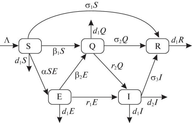
Transfer diagram of the SEQIR COVID-19 model.

Fig. 2.

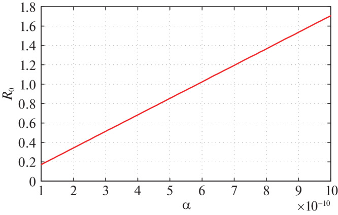
Variation of R₀ with respect to most sensitive parameter α.

Modeling of Susceptible Population (S(t))

By recruiting individuals into the region (India) at a rate Λ, the susceptible population is augmented and condensed by natural death d₁. Also the susceptible population decreases through interaction between a susceptible individual and infected but not detected by testing individual. This population is also decreased by constant rates σ₁ and β₁ respectively to be converted into quarantined individual, as well as recovered individual. It is a real fact in India especially in the districts (Purulia, Murshidabad, Birbhum (West Bengal), Gaya, Bhagalpur (Bihar), etc.) that the susceptible population is directly sent to secured zone population due to fear effect among the inhabitants. This situation arises due to lack of proper or adequate treatment or testing facility for the large number of population in India. Therefore, the rate of change of susceptible population are governed by the following differential equation:

1

Modeling of Infected but Not Detected by Testing Population (E(t))

The infected but not detected by testing population indicates those individuals who are infected but their infection is not detected due to inadequate testing facility. This population increases at a rate a by the interaction between a susceptible individual and infected but not detected by testing individual. This population decreases due to quarantine at a rate β₂ and due to natural death rate d₁. Due to very high population density, it is very difficult for the Indian Government to isolate some infected but not detected by testing individual, and send them for quarantine period. Keeping this fact in mind, let this population also directly decrease by infected population at a rate r₁. Therefore, the rate of change of infected but not detected by testing population is governed by the following differential equation:

2

Modeling of Quarantine Population (Q(t))

Incubation period for COVID-19 is 2 to 14 days. This period is very crucial for disease transformation from one individual to another individual. Therefore, we have to isolate those individual from susceptible and infected but not detected by testing individual for 14 days to control spread of COVID-19 in India. This mentioned population is known as quarantined population. Quarantined population is increased at a rate β₁ and β₂ from susceptible as well as infected but not detected by testing population respectively. This population is decreased at a rate r₂ and σ₂ due to infected population and population in secured zone correspondingly. Let the natural death rate be d₁ of this population, hence the rate of change of quarantine population is as follows:

3

Modeling of Confirmed Infected Population (I(t))

The infected population who have confirmed positive report by the COVID-19 test, is increased by infected but not detected by testing at a rate r₁ (infected but not detected by testing, such all population are not possible for quarantined due to lack of space or other reasons. Infected but not detected by testing individual may become illness for COVID-19, and subsequently their test report becomes positive. So they enter directly to the infected population, this particular case is very harmful to protect spreading COVID-19 in India), and also increased at rate r₂ from quarantined population as usual. Infected population is decreased at rate σ₃, and d₁ due to recovered population respectively. Let the natural death rate be d₁ and to make it more realistic d₂ is the rate of death for infection, and hence the rate of change of infected population is governed by the following differential equation:

4

Modeling of Secured Zone Population Not Affected by COVID-19 (R(t))

We assume that susceptible, quarantine as well as infected individuals recover from the disease at rates σ₁, σ₂ and σ₃ respectively and enter in secured zone population. This population is reduced by a natural death rate d₁. Thus, rate of change of secured zone population is not afected by COVID-19 virus is governed by the following differential equation:

5

Combining Eqs. (1)–(5) our wished-for model structure takes the following form:

6

with initial densities:

All the parameters and corresponding biological meaning are presented in Table 1 given below.

Table 1.

Explanation of parameters exploited in our proposed SEQIR model structure

Parameters	Meaning
Λ	The recruitment rate at which new individuals enter in the Indian population
α	The transmission rate from susceptible population to infected but not detected by testing population
β1	The transmission coefficient from susceptible population to quarantine population
β2	The transmission coefficient from infected but not detected by testing population to quarantine population
σ1	The transmission rate from susceptible population to secured zone population
σ2	The transmission coefficient from infected but not detected by testing population to secured zone population
σ3	The transmission rate from quarantine population to secured zone population
r 1	The transmission rate from infected but not detected by testing population to infected population for treatment
r 2	The transmission rate from quarantine population to infected population for treatment
d 2	Death rate of Infected population due to Covid-19 infection
d 1	Natural death rate of all five sub-populations

The above SEQIR model formulation (6) can be rewritten as

7

where A = (σ₁ + β₁ + d), B = (r₁ + β₂ + d₁), C = (r₂ + σ₂ + d₁) and D = (σ₃ + d₁ + d₂).

NUMERICAL VERIFICATION AND PREDICTIONS

To it our proposed COVID-19 model system (6) to the daily new COVID cases for all over India as well as five states Delhi, Kerala, Maharashtra, Uttar Pradesh and West Bengal, we performed numerical simulations in this section. Data are collected from the official website of Indian Council of Medical research and World Health Organization [47, 48]. We first estimated the values of different parameters of the model given in Table 2.

Table 2.

Values of the parameter of the model system (6) for India

Parameters	Value	Reference
Λ	4 × 104	[49]
α	4 × 10–7	Assumed
β1	0.1	Estimated
β2	5 × 10–4	Assumed
σ1	5 × 10–2	Assumed
σ2	6 × 10–3	Estimated
σ3	1 × 10–2	Estimated
r 1	1 × 10–3	Estimated
r 2	197 × 10–5	Estimated
d 2	2 × 10–5	Estimated

Initial densities as of 21th March 2020 is given in Table 3.

Table 3.

Initial densities of the model system (2.6) for India

S(0)	E(0)	Q(0)	I(0)	R(0)
8 × 108	15 × 102	5 × 104	284	4 × 108

In our proposed model system (6) most sensitive parameter is a (transmission rate from susceptible population to infected but not detected by testing population). Therefore, we mainly aspire to see the effect of on COVID-19 disease spreading. For different values of α, the value of R₀ is presented in Table 4.

Table 4.

Value of R₀ for different R₀ for India

Α	2.1 × 10–10	2.5 × 10–10	2.8 × 10–10
R 0	0.35847	0.42675	0.47796

From the above table we observe that all values of R₀ is less than unity. Hence, the endemic equilibrium E₁ is not locally asymptotically stable for these values of R₀ and corresponding α. Now we plot the graph of R₀ with respect to α.

From the above figure we observe that as the values of α increases R₀. It is also observed that after certain value of a, R₀ becomes greater than 1. Therefore, up to certain value of a DFE is stable (Theorem 3), and beyond that value of α DFE becomes unstable. In this current situation of the universe, we are interested about the infected population I(t) as days progress. Therefore, drawing the time series plot of infected population taking initial densities as given in Table 3.

Figure 3 is very interesting because we see that for α = 2.5 × 10^–10 the confirmed infected population of our proposed model system exactly fitted to the real confirmed infected individuals in India so far. To show the peak of the infection we have drawn Fig. 4 for α = 2.5 × 10^–10.

Fig. 3.

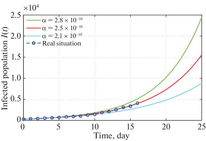
Time series plot of infected population for α = 2.8 × 10^–10, α = 2.5 × 10^–10 and α = 2.1 × 10^–10 with initial conditions, parameter values are given in Tables 2 and 3 respectively.

Fig. 4.

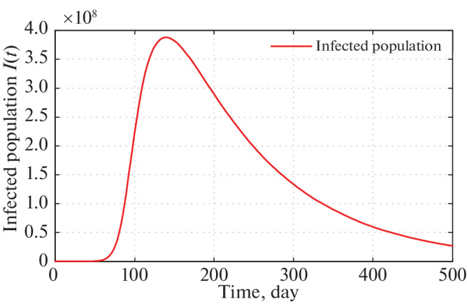
Long run time series plot of infected population for α = 2.5 × 10^–10 with initial conditions, parameter values are given in Tables 2 and 3 respectively.

Figure 4 of the infected population of our proposed model shows that, imposing the restricting measures from 21 March, 2020 by the Government of India, the peak of infection (maximum of daily cases) is attained almost after four months (120 days). After that if same restriction is continued, the peak of infection is gradually decreases.

The short time behavior of our proposed model i.e., after 30 and 60 days from the restriction measure started by the Indian Government, estimated infected individuals are depicted through Figs. 5 and 6 respectively.

Fig. 5.

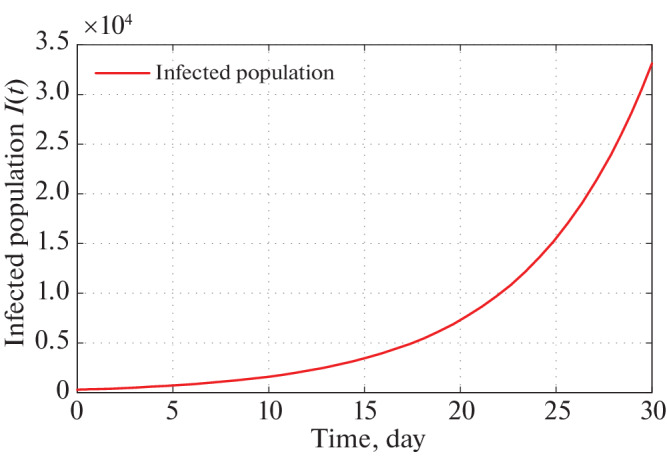
Time series plot of infected population for α = 2.5 × 10^–10 with initial conditions, parameter values are given in Tables 2 and 3 respectively for one month period.

Fig. 6.

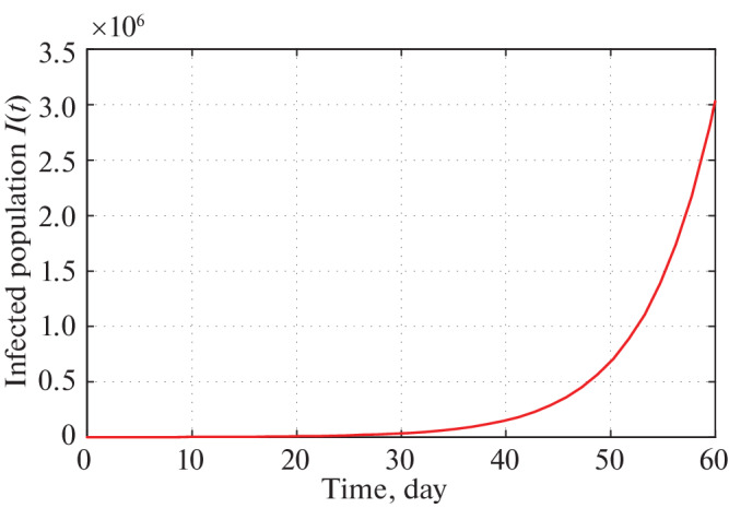
Time series plot of infected population for α = 2.5 × 10^–10 with initial conditions, parameter values are given in Tables 2 and 3 respectively for two months period.

Therefore, implementing Government restrictions mathematically, Figs. 5 and 6 infers that in 30 days number of infected individual in India goes to about 32 000. In 60 days this number goes to 3 000 000. Since, Government is changing its restricting measures after certain period of time policies, so the system parameters are also altering after that period of time. Therefore, in the current position we are not interested about infected population for long time of period.

Now, we simulate the daily new confirmed COVID-19 cases for the five states of India namely Maharashtra, Kerala, Uttar Pradesh, Delhi and West Bengal starting from 21 March, 2020. We try to it the model (6) to day by day novel confirmed COVID-19 cases in the five states of India. Here we also taken α (transmission rate from susceptible population to infected but not detected by testing population) as before. Estimated initial densities as of 21 March, 2020 are given in Table 5. Estimated Recruitment rates and infection tempted mortality rates for the dive states of India are given in Table 6. Lastly, rests of the estimated parameters are given in Table 7.

Table 5.

Estimated initial densities (as of 21 March, 2020)

State	S(0)	E(0)	Q(0)	I(0)	R(0)
Maharashtra	75 000 000	225	800	58	30 000 000
Kerala	10 000 000	200	1000	40	10 050 000
Uttar Pradesh	150 000 000	120	1500	24	50 000 000
Delhi	10 000 000	150	800	27	500 000
West Bengal	50 000 000	20	200	3	30 000 000

Table 6.

Recruitment rates and infection tempted mortality rates for the five states of India

Parameters	Maharashtra	Kerala	Uttar Pradesh	Delhi	West Bengal
Λ	3300	405	14200	650	3490
d 2	0.0032	0.00029	0.0049	0.00067	0.0024

Table 7.

Estimated parameters for the five states of India

Parameters	Maharashtra	Kerala	Uttar Pradesh	Delhi	West Bengal
β1	0.0000004	0.0000004	0.0000004	0.0000004	0.0000004
β2	0.005	0.005	0.005	0.005	0.005
σ1	0.0005	0.0005	0.0005	0.0005	0.0005
σ2	0.1	0.1	0.1	0.1	0.1
σ3	0.005	0.012	0.0038	0.0016	0.0078
r 1	0.04	0.05	0.02	0.05	0.05
r 2	0.002	0.001	0.0012	0.00093	0.0005
d 1	0.000015	0.000018	0.00002	0.00001	0.000016

Using these estimated parameters, the fixed parameters and initial densities (Tables 5–7) we graphically present infected population for different states. Figures 7 and 8 present the graphical presentation of infected population for the state Maharashtra.

Fig. 7.

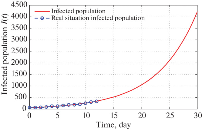
Time series plot of infected population in Maharashtra for α = 2.5 × 10^–9 using data from Tables 5–7 for one month period from 22 March, 2020.

From Fig. 7, we monitor that as per our imposed restricting measures as given by Government of India, total number of infected individuals in Maharashtra reaches to 4100 in 30 days from 21 March, 2020. We also detect from Fig. 7 that the actual number of infected persons also coincides with the infected COVID-19 individuals of our proposed system for 13 days starting from 21 March, 2020. Again Fig. 8 infers that total number of infected population reaches to 260 000 in two months. But in reality this situation may not happen as Government is continuously changing its restricting measures to stop the spreading of COVID-19.

Fig. 8.

Time series plot of infected population in Maharashtra for α = 2.5 × 10^–9 using data from Tables 5–7 for two months period from 22 March, 2020.

Now to illustrate the COVID-19 situation in Kerala based on values of parameters as given in Tables 5–7 we draw the following two figures.

Figure 9 shows that in 30 days the infected population of Kerala reached to 2100. Also we have observed real infected individual for 13 days overlap with our infected population curve. Figure 10 shows that the infected individuals in Kerala go to 50 000 in 60 days from 21 March, 2020. But recent trends show that the infected individuals are far less than our expected number. This is because Kerala Government has taken proper strict preventing measures to stop spreading COVID-19 virus.

Fig. 9.

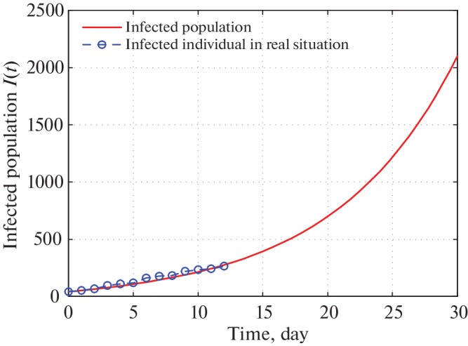
Time series plot of infected population in Kerala for α = 0.0000000164 using data from Tables 5–7 for one month period from 22 March, 2020.

Fig. 10.

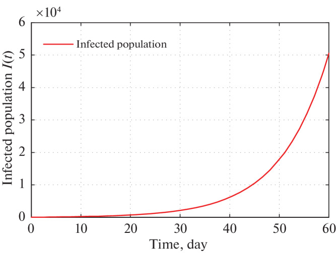
Time series plot of infected population in Kerala for α = 0.0000000164 using data from Tables 5–7 for two months period from 22 March, 2020.

Following two figures gives the situation of COVID-19 in Uttar Pradesh.

Figures 11 and 12 depict that as per our construction infected population in 30 and 60 days are 4400 and 620 000 respectively starting from 21 March, 2020.

Fig. 11.

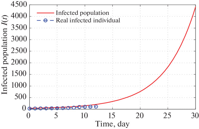
Time series plot of infected population in Uttar Pradesh for α = 0.000000020 using data from Tables 5–7 for one month period from 22 March, 2020.

Fig. 12.

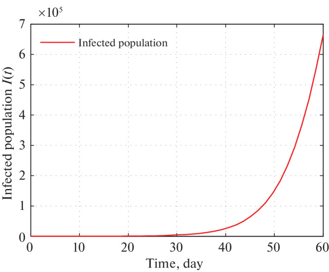
Time series plot of infected population in Uttar Pradesh for α = 0.000000020 using data from Tables 5–7 for two months period from 22 March, 2020.

Similarly, for the state Delhi we draw the following two figures.

Figures 13 and 14 depict that as per our construction infected population in Delhi during 30 and 60 days are 4600 and 400 000 respectively starting from 21 March, 2020.

Fig. 13.

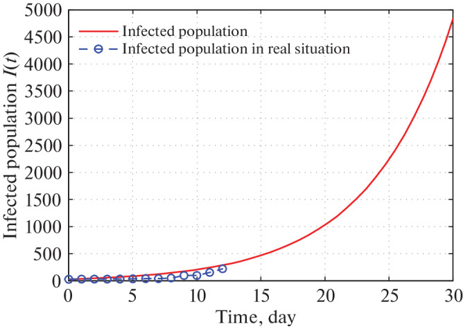
Time series plot of infected population in Delhi for α = 0.000000021 with initial conditions, parameter values are given in Tables 5–7 respectively for one month period from 21 March, 2020.

Fig. 14.

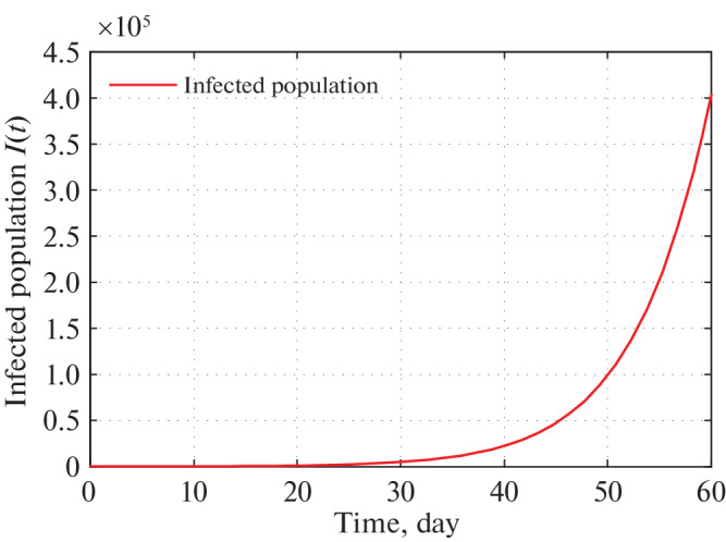
Time series plot of infected population in Delhi for α = 0.000000021 using data from Tables 5–7 for two month period from 21 March, 2020.

Finally COVID-19 pandemic situation in West Bengal can be expressed by the following two figures.

As before Figs. 15 and 16 infer that as per our construction infected population in West Bengal during 30 and 60 days are 1100 and 210 000 respectively starting from 21 March, 2020.

Fig. 15.

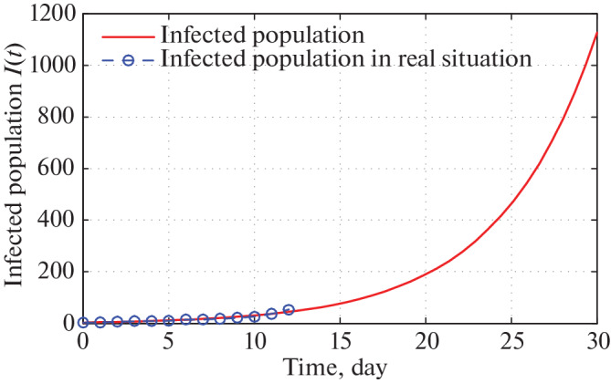
Time series plot of infected population in West Bengal for α = 0.0000000047 with initial conditions, parameter values are given in Tables 5–7 respectively for one month period from 21 March, 2020.

Fig. 16.

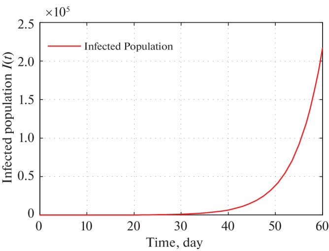
Time series plot of infected population in West Bengal for α = 0.0000000047 using data from Tables 5–7 for two months period from 21 March, 2020.

CONCLUSION AND DISCUSSION

In this current paper we have formulated and studied an epidemic model of COVID-19 virus which is transferred from human to human. So far the daily confirmed COVID-19 cases are increasing day by day worldwide. Therefore, prediction about infected individual is very much important for health concern arrangement of the citizens. It is also important to control spread rate of the COVID-19 virus with restricted supply. Our mathematical study is based on COVID-19 virus spread in India. We try to fit our model system to COVID-19 disease in India as per as limited data are available. The basic reproduction number R₀ is calculated of our anticipated model. It is observed that when R₀ < 1 then DFE E₀ is globally asymptotically stable. Again, from sensitivity analysis of R₀ we observe that the most sensitive parameter of our model structure is a (transmission rate from susceptible population to infected but not detected by testing population). Also the endemic equilibrium E₁ exist and stable if R₀ > 1.

In this study our main aim is to predict mathematically the number of infected individual due COVID-19 virus in India. To fulfill our aim, we perform a detail numerical simulation of our proposed model in Section 6. We first simulate the COVID-19 situation in India, and thereafter situation of five different states (Maharashtra, Kerala, Uttar Pradesh, Delhi and West Bengal) are predicted numerically through graphical approach using Matlab software. We estimated the values of the parameter and the initial condition taken as per the information accessible on 21 March 2020.

We see that a is most sensitive parameter of our model system. So for different values of a infected population curve is presented in Fig. 3. We observe that for α = 2.5 × 10^–10, the infected population curve is best fitted since it coincides with the actual infected individuals for 13 days starting from 21 March, 2020. Long term behavior of the infection is observed in Fig. 4. This figure shows us that as per the model construction as well as data available, the peak of infection is reached about 120 days after 21 march, 2020. Therefore, as per our prediction, the estimated date to reach the peak of infection is 21 July 2020 if the same restriction of measures is followed by the Indian Government as declared on 21 March 2020. Short term prediction about infected population is given via Figs. 5 and 6 respectively. Accordingly two of these figures predicted number of infected individual in India of COVID-19 patients in 30 and 60 days are 32 000 and 3 000 000 respectively starting from 21 March 2020.

Now, we look upon the situation of different states. Figures 7 and 8 present that the number of infected population reaches to 4100 and 260 000 (for α = 2.5 × 10^–9) in next 30 and 60 days respectively starting from 21 March, 2020. For Kerala this number goes to 2100 and 50  000 (for α = 0.0000000164) respectively (see Figs.9 and 10). In Uttar Pradesh, as per Figs. 11 and 12 (for α = 0.000000020) predicted numbers of infected individuals are 4400 and 620 000. Total numbers of 4600 and 400 000 people are infected in 30 and 60 days respectively in Delhi (look at Figs. 13 and 14). Finally, in West Bengal 1100 and 210 000 people may be infected due to COVID-19 virus in 30 and 60 days respectively (see Figs. 15 and 16).

Therefore, analyzing all results of our proposed model and observing the situation of different countries, we may conclude that India may be in a big trouble in very near future due to COVID-19 virus. To avoid this big trouble, Indian Government should take stricter measures other than quarantine, lock down etc. So far the Indian Government are continuously changing its policy to protect India from COVID-19 virus. Recently, all districts of India are classified by Indian Government into three zones namely Red zones (hotspots), Orange zones (non hotspots) and Green zones (save zones). Preliminarily 170 districts of India are hotspots zones, where rapid testing facility is available for the public. As the time progress more strategies are applied by the Government of India as well as all state Governments to stop the spread of COVID-19 virus in India. Therefore, we may assume that if the Indian Government take proper step time to time then the infected number of population will be differ from our predicted number as time progress, and India will recover from this virus in recent future. Lastly, we say that public of India should help the Indian Government to fight against this dangerous COVID-19 as per the proposed model.

APPENDIX A

BASIC PROPERTIES

Non Negativity of Solution

Theorem 1 (A1). Each solution of the SEQIR model structure (7) with preliminary stipulations subsists in the interval [0, ∞) and S(t) > 0, E(t) ≥ 0, I(t) ≥ 0 as well as R(t) > 0 for all values t greater than equal to zero.

Proof. As the right hand side of SEQIR model structure (7) is completely continuous and locally Lipschitzian on C, the solution (S(t), E(t), I(t), R(t)) of (7) with initial conditions exists, and is unique on [0, ξ), where 0 < ξ < +∞.

From system (7) with initial condition, we have

The second equation of system (7), implies dE/dt ≥ –BE(t).

Using initial condition we obtain E(t) ≥ E(0)exp[–Bt] ≥ 0.

Again from third and fourth equations of the system (7) with the help of initial condition provide

Furthermore, last equation of (7) provides dR/dt ≥ –d₁R → R(t) ≥ R(0)exp[–d₁t] > 0.

Therefore, we can see that S(t) > 0, E(t) ≥ 0, I(t) ≥ 0, R(t) > 0, ∀t ≥ 0. This concludes the proof of the theorem.

Invariant Region

Theorem 2 (A2). All solutions of the SEQIR model structure (7) that initiate in are bounded and enter into a region Ω defined by Ω = {(S, E, Q, I, R) ∈ : 0 < N(t) ≤ Λ/ζ} as t → ∞, where ζ = min{d₁, d₁ + d₂}.

Proof. Suppose N(t) = S(t) + E(t) + I(t) + R(t), where (S(t), E(t), Q(t), I(t), R(t)) SEQIR model structure (7). Differentiating both sides with respect to t, we have

After substitute the values of dS(t)/dt, dE(t)/dt, dQ(t)/dt, dI(t)/dt, and dR(t)/dt from Eq. (7), we obtain

Now

where ζ = min{d₁, d₁ + d₂}. Now by using comparison theorem, we obtain

As t → ∞, we have 0 < N(t) ≤ Λ/ζ. Therefore, all solution of the model structure (7) enter in the region Ω = {(S, E, Q, I, R) ∈ : 0 < N(t) ≤ Λ/ζ}. Hence, we have completed the required proof.

APPENDIX B

DISEASES-FREE EQUILIBRIUM AND THE BASIC REPRODUCTION NUMBER

The diseases-free equilibrium (DFE) of the proposed SEQIR model (7) is acquired by setting E = 0, Q = 0, I = 0 and R = 0. The obtained DFE is E₀(Λ/A, 0, 0, 0, 0).

Basic Reproduction Number (BRN) [39–42] is a number which is defined as the new infective formed by a solitary infective individual for the duration of his or her effectual infectious epoch when introduced into an utterly susceptible populace at equilibrium.

To find the BRN of our proposed SEQIR model structure (7), we take the assistance of next-generation matrix method [41] formulation. Assume y = (E, Q, I, R, S)^T, then the system (7) can be rewritten as

where 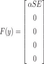and .

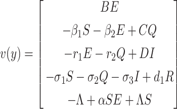F is known as transmission part which, articulates the production of new infection and is known as transition part, which explain the alter in state.

The Jacobian matrices of F(y) and (y) at the DFE E₀ is given by

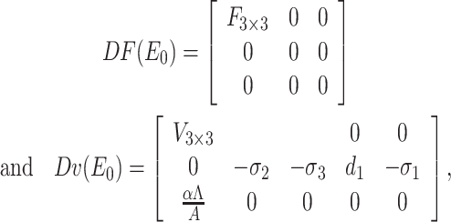where F = 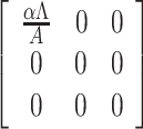and V = .

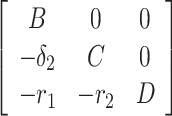Therefore, FV^–1 is the next generation matrix of the SEQIR model structure (7). So, as per [41] R₀ = ρ(FV^–1) where ρ stands for spectral radius of the next-generation matrix FV^–1. Therefore,

It is notable that L/A represents the number of susceptible individual at the DFE E₀.

SENSITIVITY ANALYSIS OF R₀

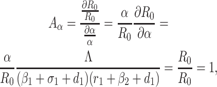
Based on the each of the parameters of R₀ a sensitivity analysis is performed to check the sensitivity of the basic reproduction number. As indicated by Arriola and Hyman [43] we have computed the normalized forward sensitivity index with respect to each of the parameters

B.1

From the above calculations, it is obvious that the BRN R₀ is mainly sensitive to alters in α. The value of R₀ will be enhanced if we raise the value of α. On the contrary, the value of R₀ will be as well reduced in the same proportion if we diminish the value of α. Again it is also noticed that the parameters β₁, σ₁, d₁, r₁ and β₂ are related to R₀ inversely. Therefore, for any increasing value of any of this mentioned parameters will definitely reduce the value of R₀. But the decreasing value of R₀ will be comparatively slighter. Since the effect of parameters β₁, σ₁, d₁, r₁ and β₂ are very small on R₀, it will be sensible to focus efforts on the reduction of α (transmission rate at which the susceptible individual converted to exposed individual). Therefore, the sensitive analysis of the basic reproduction number emphasized that prevention is better than treatment. That is exertions to enhance prevention are further effective in controlling the spread of COVID-19 disease than to enlarge the numbers of individuals accessing treatment, as yet there is no proper vaccine, which is medically proven this technique is very much effective to control the spread of Coronavirus disease in country like India. Following the same concept, the Indian Government as well as all State Government of India have taken necessary action such as Lockdown, campaign against the disease etc. to protect the out break of this dangerous disease.

STABILITY ANALYSIS OF DISEASES-FREE EQUILIBRIUM

This section is constructed with an aim to study the stability nature of the Diseases Free Equilibrium (DFE) E₀ with the assistance of subsequent Theorems:

Theorem 3. The SEQIR model structure (7) at DFE E₀(Λ/A, 0, 0, 0, 0) is locally asymptotically stable under the condition R₀ < 1 and became unstable if R₀ > 1.

Proof. The Jacobian of the system (7) at DFE E₀(Λ/A, 0, 0, 0, 0) is given by

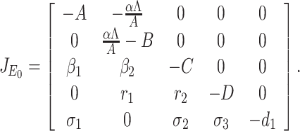The characteristic equation of the matrix is given

B.2

where λ is a eigenvalue of the matrix . Therefore, roots of Eq. (B.2) i.e., eigenvalues of the matrix are λ₁ = –A < 0, λ₂ = αΛ/A – B, λ₃ = –C < 0, λ₄ = –D < 0 as well as λ₅ = –d₁ < 0. Therefore, Therefore the system (7) is locally asymptotically at the DFE E₀(Λ/A, 0, 0, 0, 0) if λ₂ < 0. Now λ₂ < 0 implies

Hence, DEF E₀(Λ/A, 0, 0, 0, 0) is locally asymptotically stable under the condition R₀ < 1.

Theorem 4. The SEQIR model structure (7) at DFE E₀(Λ/A, 0, 0, 0, 0) is globally asymptotically stable (GAS) under the condition R₀ < 1 and became unstable if R₀ > 1.

Proof. We can rewrite the system of differential Eq. (7) in the following form given below

Here, X = (S, R) ∈ R ² (the number of uninfected individuals compartments), V = (E, Q, R) ∈ R ³ (the number of infected individuals compartments) as well as E₀(Λ/A, 0, 0, 0, 0) is the DFE of the SEQIR model structure (7). DFE Eo is globally stable if the subsequent two stipulations are fulfilled:

(1) For dX/dt = F(X, V), X* is globally asymptotically stable,

(2) , for ,

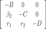where B = D_VG(X*, 0), is a Metzler matrix and Ω is the positively invariant set with respect to the model (7). Following Castillo-Chavez et al. [44], we check for aforementioned conditions. For our proposed model structure (7) F(X, 0) = , B = and (X, V) = .

Obviously, (X, V) ≥ 0 every time the state variables are within Ω. It is also obvious that X* = (Λ/A, 0) is a globally asymptotically stable equilibrium of the system dX/dt = F(X, 0). Hence, the theorem is proved.

APPENDIX C

EXISTENCE OF ENDEMIC EQUILIBRIUM POINT AND ITS STABILITY

This section reflects the existence of endemic equilibrium as well as demonstrates its stability nature. To stumble on the endemic equilibrium E₁(S*, E*, Q*, I*, R*) of our wished-for SEQIR structure (7) we deem the following:

as well as

C.1

Solving the system of Eq. (C.1) we obtain

From first equation of (C.1) we have

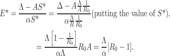Therefore, E* has unique positive value if R₀ – 1 > 0 i.e., R₀ > 1. Shortening the above discussions and discussions in the previous sections we have reached the following theorem:

Theorem 5 (C.1). The SEQIR model structure (7) has a unique DFE E₀(Λ/A, 0, 0, 0, 0) for all parameter values as well as the system (7) has also a unique endemic equilibrium E₁(S*, E*, Q*, I*, R*) under the condition R₀ > 1.

The next theorem establish the local stability nature of the endemic equilibrium E₁(S*, E*, Q*, I*, R*)

C.2

We assume α* = α, as the bifurcation parameter, predominantly as it has been explained in (B.1) that R₀ is extra sensitive to alter in than the other parameters. If it is considered that R₀ = 1, then we have

C.3

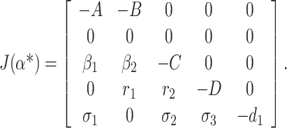
Now, the Jacobian of the linearized system (C.1) via (C.2) at DFE E₀ when α* = α is as follows:

C.4

Eigenvalues of the matrix (C.4) are given by (0, –A, –C, –D, –d₁)^T. We observe that the matrix (C.4) has simple zero eigenvalue, and the other eigenvalues are negative. We are now at the stage to apply center manifold theory [45] to analyze the dynamics of system (C.1). Corresponding to zero eigenvalue the right eigenvector ω = (ω₁, ω₂, ω₃, ω₄, ω₅)^T of the matrix (C.4) is given by

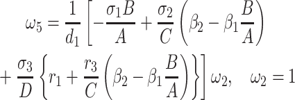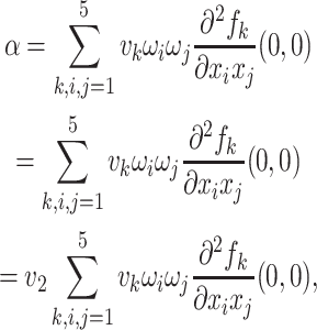
with ω₂ free. Moreover, J(a*) has a corresponding left eigen vector = (₁, ₂, ₃, ₄, ₅) where ₁ = 0, ₂ = 0, ₃ = 0, ₄ = 0, ₅ = 0 with ₂ free. Therefore, we have

Substituting the values of all the second-order derivatives calculated at DFE as well as α* = α we obtain,

As a < 0 and b > 0 at α* = α, hence, from Remark 1 of Theorem 4.1 as declared in [44], a transcritical bifurcation takes place at R₀ = 1 as well as the inimitable endemic equilibrium is locally asymptotically stable due to R₀ > 1. Hence, we conclude the proof.

COMPLIANCE WITH ETHICAL STANDARDS

Conflict of interest. The authors declare that they have no conflicts of interest.

Statement on the welfare of humans or animals. This article does not contain any studies involving animals performed by any of the authors.

REFERENCES

- 1.Huang Y., Li X. Lancet. 2020;395:497. doi: 10.1016/S0140-6736(20)30183-5. [DOI] [PMC free article] [PubMed] [Google Scholar]
- 2.Zhu N., Zhang D., Wang W., Li X. New Engl. J. Med. 2020;382:727. doi: 10.1056/NEJMoa2001017. [DOI] [PMC free article] [PubMed] [Google Scholar]
- 3.National Health Commission of the People’s Republic of China. http://www.nhc.gov.cn/xcs/yqfkdt/202004/ be27dc3c4a9544b081e2233537e762c3.shtml. Accessed April 2, 2020.
- 4.Gumel A. B, Ruan S., Day T. Proc. R. Soc. London, Ser. B. 2004;271:2223. doi: 10.1098/rspb.2004.2800. [DOI] [PMC free article] [PubMed] [Google Scholar]
- 5.Li W., Moore M. J., Vasilieva N. Nature. 2003;426:450. doi: 10.1038/nature02145. [DOI] [PMC free article] [PubMed] [Google Scholar]
- 6.Groot R. J., Baker S. C., Baric R. S. J. Virol. 2013;87:7790. doi: 10.1128/JVI.01244-13. [DOI] [PMC free article] [PubMed] [Google Scholar]
- 7.Wit E., Doremalen N., Falzarano D., Munster V. J. Nat. Rev. Microbiol. 2016;14:523. doi: 10.1038/nrmicro.2016.81. [DOI] [PMC free article] [PubMed] [Google Scholar]
- 8.Cowling B. J., Park M., Fang V. J. Eurosurveillance. 2015;20:21163. doi: 10.2807/1560-7917.ES2015.20.25.21163. [DOI] [PMC free article] [PubMed] [Google Scholar]
- 9.Gralinski L. E, Menachery V. D. Viruses. 2020;12:135. doi: 10.3390/v12020135. [DOI] [PMC free article] [PubMed] [Google Scholar]
- 10.Centers for Disease Control and Prevention: 2019 Novel Coronavirus. https://www.cdc.gov/coronavirus/2019-ncov, 2020. Accessed March 10, 2020.
- 11.Fuk-Woo Chan J., Yuan S., Kok K. Lancet. 2020;395:514. doi: 10.1016/S0140-6736(20)30154-9. [DOI] [PMC free article] [PubMed] [Google Scholar]
- 12.Cheng Z. J, Shan J. Infection. 2020;48:155. doi: 10.1007/s15010-020-01401-y. [DOI] [PMC free article] [PubMed] [Google Scholar]
- 13.Coronavirus Disease (COVID-19) Situation Dashboard, World Health Organization, 2020. https://experience.arcgis.com/experience/685d0ace521648f8a5beeeee1b9125cd. Accessed April 2, 2020.
- 14.Coronavirus disease 2019 (COVID-19) Situation Report–73, World Health Organization, 2020, https://www.who.int/docs/default-source/coronaviruse/situation-reports/20200402-sitrep-73-covid-19.pdf?sfvrsn=5ae25bc7_2, Accessed April 2, 2020.
- 15.Timeline of the 2020 Coronavirus Pandemic in India, 2020. https://en.wikipedia.org/wiki/Timeline_of_the_ 2020_coronavirus_pandemic_in_India#January. Accessed April 2, 2020.
- 16.Ministry of Health and Family Welfare, Government of India 2020. https://www.mohfw.gov.in/. Accessed April 3, 2020.
- 17.2020 Coronavirus Pandemic in India, 2020. https://en.wikipedia.org/wiki/2020_coronavirus_pandemic_in_India#cite_note-: 2–10. Accessed April 3, 2020.
- 18.WHO Statement on the Second Meeting of the International Health Regulations (2005) Emergency Committee Regarding the Outbreak of Novel Coronavirus (2019-ncov) (World Health Organization, Geneva, 2020). https://www.who.int/. Accessed September 4, 2020.
- 19.Rivers C., Chretien J. P., Riley S. Nat. Commun. 2019;10:3102. doi: 10.1038/s41467-019-11067-2. [DOI] [PMC free article] [PubMed] [Google Scholar]
- 20.Chowell G., Bertozzi S. M., Colchero M. A. New Engl. J. Med. 2009;361:674. doi: 10.1056/NEJMoa0904023. [DOI] [PubMed] [Google Scholar]
- 21.Chowell G., Echevarria-Zuno S., Viboud C. PLoS Med. 2011;8:e1000436. doi: 10.1371/journal.pmed.1000436. [DOI] [PMC free article] [PubMed] [Google Scholar]
- 22.Fraser C., Donnelly C. A., Cauchemez S. Science. 2009;324:1557. doi: 10.1126/science.1176062. [DOI] [PMC free article] [PubMed] [Google Scholar]
- 23.Lipsitch M., Cohen T., Cooper B. Science. 2003;300:1966. doi: 10.1126/science.1086616. [DOI] [PMC free article] [PubMed] [Google Scholar]
- 24.Kucharski A. J., Russell T. W., Diamond C. Lancet. Infect. Dis. 2020;20:553. [Google Scholar]
- 25.J. M. Read, J. R. E. Bridgen, D. AT. Cummings, et al., Philos. Trans. R. Soc., B 376, 20200265 (2021). 10.1098/rstb.2020.0265 [DOI] [PMC free article] [PubMed]
- 26.Tang B., Wang X., Li Q. J. Clin. Med. 2020;9:462. doi: 10.3390/jcm9020462. [DOI] [Google Scholar]
- 27.T. Zeng, Y. Zhang, Z. Li, et al., arXiv:2002.04945 [q-bio.PE] (2020). 10.48550/arXiv.2002.04945.
- 28.Huang N. E., Qiao F. Sci. Bull. 2020;65:425. doi: 10.1016/j.scib.2020.02.005. [DOI] [PMC free article] [PubMed] [Google Scholar]
- 29.S. Lai, I. Bogoch, N. Ruktanonchai, A. Watts, et al., medRxiv 2020.02.04.20020479 (2020). https://doi.org/10.1101/2020.02.04.20020479
- 30.K. Muniz-Rodriguez, G. Chowell, C. Cheung, et al., medRxiv 2020.02.05.20020750 (2020). https://doi.org/10.1101/2020.02.05.20020750
- 31.Nowcasting and Forecasting the Wuhan 2019-nCoV Outbreak (2020). https://.les.sph.hku.hk/download/wuhan_exportation_preprint.pdf. Accessed September 4, 2020.
- 32.Wu J. T., Leung K., Leung G. M. Lancet. 2020;395:689. doi: 10.1016/S0140-6736(20)30260-9. [DOI] [PMC free article] [PubMed] [Google Scholar]
- 33.Imai N., Cori A., Dorigatti I. Report 3: Transmissibility of 2019-nCoV. 2020. [Google Scholar]
- 34.Volpert V., Banerjee M., Petrovskii S. Nat. Phenom. 2020;15:24. doi: 10.1051/mmnp/2020006. [DOI] [Google Scholar]
- 35.May R. M. Infectious Diseases of Humans: Dynamics and Control. 1991. [Google Scholar]
- 36.Diekmann O., Peter Heesterbeek J. A. Mathematical Epidemiology of Infectious Diseases: Model Building, Analysis and Interpretation. New York: Wiley; 2000. [Google Scholar]
- 37.Hethcote H. W. SIAM Rev. 2000;42:599. doi: 10.1137/S0036144500371907. [DOI] [Google Scholar]
- 38.Sharma S., Samanta G. P. J. Biol. Syst. 2014;22:713. doi: 10.1142/S0218339014500296. [DOI] [Google Scholar]
- 39.Anderson R. M., May R. M. Nature. 1979;280:361. doi: 10.1038/280361a0. [DOI] [PubMed] [Google Scholar]
- 40.Brauer F., Castillo-Chavez C. Mathematical Models in Population Biology and Epidemiology. Berlin: Springer; 2001. [Google Scholar]
- 41.Van Den Driessche P., Watmough J. Math. Biosci. 2002;180:29. doi: 10.1016/S0025-5564(02)00108-6. [DOI] [PubMed] [Google Scholar]
- 42.Nyabadza F., Hove-Musekwa S. D. Math. Biosci. 2010;225:132. doi: 10.1016/j.mbs.2010.03.002. [DOI] [PubMed] [Google Scholar]
- 43.Arriola L., Hyman J. Lecture Notes: Forward and Adjoint Sensitivity Analysis with Applications in Dynamical Systems, Linear Algebra and Optimization. 2005. [Google Scholar]
- 44.C. Castillo-Chavez, Zh. Feng, and W. Huang. On the Computation of R(o) and Its Role on Global Stability, Biometrics Unit Technical Report No. BU-1553-M (Cornell Univ., New York, 2002).
- 45.Carr J. Applications of Center Manifold Theory. New York: Springer; 1981. [Google Scholar]
- 46.Castillo-Chavez C., Song B. Math. Biosci. Eng. 2004;1:361. doi: 10.3934/mbe.2004.1.361. [DOI] [PubMed] [Google Scholar]
- 47.WHO. Coronavirus Disease (COVID-19) Outbreak (2019). https://www.who.int/emergencies/diseases/novel coronavirus-2019. Accessed April 14, 2020.
- 48.Indian Council of Medical Research (2019). https://www.icmr.nic.in/. Accessed April 14, 2020.
- 49.India Birth Rate, 1950–2021. https://knoema.com/atlas/India/Birth-rate. Accessed April 8, 2020.