How to Model and Interpret Cross-Lagged Effects in Psychotherapy Mechanisms of Change Research: A Comparison of Multilevel and Structural Equation Models

Abstract

Objective:

Modeling cross-lagged effects in psychotherapy mechanisms of change studies is complex and requires careful attention to model selection and interpretation. However, there is a lack of field-specific guidelines. We aimed to (a) describe the estimation and interpretation of cross lagged effects using multilevel models (MLM) and random-intercept cross lagged panel model (RI-CLPM); (b) compare these models’ performance and risk of bias using simulations and an applied research example to formulate recommendations for practice.

Method:

Part 1 is a tutorial focused on introducing/describing dynamic effects in the form of autoregression and bidirectionality. In Part 2, we compare the estimation of cross-lagged effects in RI-CLPM, which takes dynamic effects into account, with three commonly used MLMs that cannot accommodate dynamics. In Part 3, we describe a Monte Carlo simulation study testing model performance of RI-CLPM and MLM under realistic conditions for psychotherapy mechanisms of change studies.

Results:

Our findings suggested that all three MLMs resulted in severely biased estimates of cross-lagged effects when dynamic effects were present in the data, with some experimental conditions generating statistically significant estimates in the wrong direction. MLMs performed comparably well only in conditions which are conceptually unrealistic for psychotherapy mechanisms of change research (i.e., no inertia in variables and no bidirectional effects).

Discussion:

Based on conceptual fit and our simulation results, we strongly recommend using fully dynamic structural equation modeling models, such as the RI-CLPM, rather than static, unidirectional regression models (e.g., MLM) to study cross-lagged effects in mechanisms of change research.

The study of mechanisms of change in psychotherapy is advancing rapidly, with the more regular use of repeated measurement (e.g., session-by-session assessments) and advances in statistical analysis methods. Contemporary versions of the cross-lagged panel model (CLPM; Allison et al., 2017; Curran et al., 2014; Hamaker et al., 2015; Zyphur, Allison, et al., 2020; Zyphur, Voelkle, et al., 2020), estimated using structural equation modeling (SEM; Kline, 2016), are increasingly being used to model candidate mechanisms of change and their relationships to outcome. These models are complex and challenging to interpret, with the effect that psychotherapy researchers often choose simpler, regression-based models—usually estimated using multilevel models (MLM; Snijders & Bosker, 2012). There are many examples, including some of our own previous publications (e.g., Braun et al., 2015; Chen et al., 2020; Conklin & Strunk, 2015; Falkenström et al., 2013; Flückiger et al., 2020; Gómez Penedo et al., 2020; Øktedalen et al., 2015; Rubel, Bar-Kalifa, et al., 2018; Rubel et al., 2017; Rubel, Zilcha-Mano, et al., 2018; Zilcha-Mano et al., 2014, 2016). The aims of this paper are to (a) describe important differences between these two classes of models (SEM vs. MLM), focusing on their conceptual interpretation in the context of psychotherapy mechanisms of change research and (b) explore the performance of MLM using a simulation study when data is generated in accordance with the more flexible SEM specifications, which we believe represent more realistic conditions in psychotherapy mechanisms of change research. In these settings, mechanisms and outcome are typically measured repeatedly during treatment (often weekly, or session-by-session), to test whether candidate mechanisms predict outcome over the course of psychotherapy. First, however, we will briefly introduce the issue of within- and between patient variation, which is important for contemporary mechanisms of change research.

Within-Patient Changes and Between-Patient Differences

Panel data¹ includes repeated measures on multiple patients over time and has important advantages: it enables greater generalizability with fewer data-points compared to a single-case study, while providing greater confidence in causal inference than cross-sectional data due to the possibility of determining temporal precedence. However, panel data also introduces increased complexity. It includes both variation over time within individuals and cross-sectional variation, that is, differences between individuals. Several authors have argued that these sources of variation need to be separated (e.g., Curran & Bauer, 2011; Hamaker, 2012; Wang & Maxwell, 2015), and that effects should be estimated on a within-patient level after removing stable average differences between individuals (Hamaker et al., 2015) and/or linear changes over time (Curran et al., 2014). Within-patient analyses come with the advantage of allowing firmer causal inference, since these associations are, in principle, unaffected by any potential confounders that are stable (or change linearly) over time (e.g., Falkenström et al., 2017, 2020b). In addition, a within-patient focus fits with psychotherapy mechanisms of change research, which focuses on predictions of change within individuals. For instance, in mechanisms of change research, we may be interested in whether a patient who experiences fewer negative cognitions than usual in one session shows improved depression severity at the following session (within-patient cross-lagged effect). We would probably be less interested in, or at least find it more difficult to interpret, a result showing that patients with fewer negative cognitions than other patients in the study are more likely to improve their position on a depression measure relative to other patients in the study at the next session (cross-lagged effect without separation of within- from between person variances). Another problem with between-patient effects lies in the fact that any additional differences between patients can have confounding effects on the relationship between cognitive change (CC) and depressive symptoms.

In Part 1, we introduce the within-patient level of the random intercept cross-lagged panel model (RI-CLPM; Hamaker et al., 2015). There are several contemporary versions of CLPM that handle within/between patient separation in slightly different ways, for instance, the latent curve model with structured residuals (Curran et al., 2014), the maximum likelihood structural equation model (Allison et al., 2017), and the general cross-lagged panel model (Zyphur, Allison, et al., 2020; Zyphur, Voelkle, et al., 2020). We focus on the RI-CLPM because its interpretation is straightforward, but many of our arguments apply to the other models as well. In Part 2, we will describe how to separate within-patient fluctuations from stable between-patient differences. Finally, in Part 3, we present the results of a simulation study showing the effects of using multilevel regression models on data generated from the more complex RI-CLPM structure, which is better aligned with clinical theories about mechanisms of change.

Part 1: Introducing the Within-Patient Part of the Random Intercept Cross-Lagged Panel Model

When choosing a statistical analysis method, it is important to first reflect on the relevance of its assumptions to the real-world processes a researcher attempts to model. In applied research, the true data-generating process is unknown, although researchers familiar with the study subject can make educated guesses about the nature of this process. Therefore, knowing the assumptions of each model is crucial for evaluating to what extent these seem realistic in a given context. We will first describe the assumed data-generating process of the RI-CLPM. Later, we will compare these assumptions with those of regression based MLM models. The assumptions underlying the models are evaluated with regard to their fit to clinical theories about how change unfolds in the process of psychotherapy.

Throughout Part 1, we will use an applied example from a published study (Fitzpatrick et al., 2020) which investigated the effect of a candidate mechanism of change, negative cognitions, on depression severity over the course of cognitive behavioral therapy (CBT). The mechanism was operationalized as CC, measured by the Immediate Cognitive Change Scale (Fitzpatrick et al., 2020) after each session. Depression severity, measured at the start of each session, was measured using the Beck Depression Inventory (BDI; Beck et al., 1961).

Figure 1 depicts the full RI-CLPM. In the following paragraphs, we will focus on the assumptions of the within-patient part of this model. In Part 2, we will compare these assumptions to the ones made in multilevel models that in psychotherapy research are often used to analyze similar research questions. Because we want to focus on the within-patient part, we will assume a very simple between-patient structure; such that patients differ only in their average levels of depressive symptoms. Longer-term trends in means over time (Curran & Bauer, 2011) are important but beyond the scope of this inquiry.

Figure 1. Four-Wave Random Intercept Cross-Lagged Panel Model (Hamaker et al., 2015).

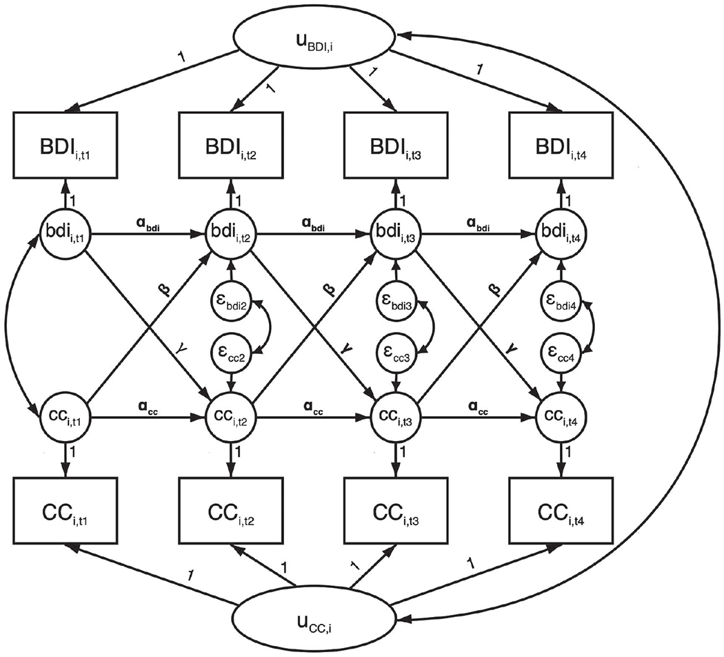
Note. Observed variables (boxes) are separated into latent between-person variables (u_BDI,i and u_CC,i) and within-person deviation scores (small circles, bdi_i,t and cc_i,t). Auto- (α_bdi and α_cc) and cross-lagged (β and γ) regressions are estimated among within-person deviation scores. Between-person variables, and within-person variables at the same time-point, are allowed to correlate. BDI = Beck Depression Inventory; CC = cognitive change.

The Autoregressive Effect

In Figure 1, observed variables are written in capital letters, while latent within-patient deviation variables are written in lower-case letters. In Figure 2, we have taken the within-patient part of Figure 1 and split it up into four potential within-patient models, to clearly show the various components of the within-patient part of the model. Figure 2a shows within-patient depressive symptoms (bdi) session-by-session, with effects derived from our study example. The arrows, or paths, going from bdi₁ to bdi₂ to bdi₃, and so on, are called autoregressive effects. The autoregressive effects indicate the proportion of bdi variance that is carried forward to later measurement occasions, that is, how much of the session-to-session fluctuations in depression severity can be explained by knowing depression severity of the previous week. Conceptually, this can be understood as inertia, that is, the autoregressive paths indicate the extent to which depressive symptoms tend to linger on from one session to the next. The assumption when modeling autoregression is that depression severity at one time-point causes depression severity at the next time-point (Rabe-Hesketh & Skrondal, 2012). For instance, depressed individuals experience reduced motivation to engage in pleasurable activities, which maintains isolation and exacerbates low motivation (Carvalho & Hopko, 2011). Similarly, anxious individuals tend to avoid potentially stressful situations, which in turn may sustain symptomatology. A general equation for such an autoregressive process would be as follows: bdi_t = α × bdi_t−1 + ε_t.

Figure 2. Components of the Within-Patient Part of the Random Intercept Cross-Lagged Panel Model (RI-CLMP).

Note. Model (a) shows an autoregressive process in BDI, (b) adds predictor CC to arrive at a dynamic panel model, (c) adds feedback from BDI to CC, and (d) is a fully bivariate CLPM, including autoregression in CC. BDI = Beck Depression Inventory; CC = cognitive change; CLPM = cross-lagged panel model.

In this equation, α is the autoregression coefficient, and ε_t is the error term at time t (i.e., that part of the variation in bdi_t which cannot be explained by the autoregressive effect). To see how this model works, it is easier to look at the equations for each time-point separately. Thus, the equation for depression severity at Session 2 is bdi₂ = α × bdi₁ + ε₂. If α is equal to 1, all the severity from Session 1 (bdi₁) would be carried forward to Session 2 (bdi₂), indicating strong inertia of symptoms. Conversely, if α = 0, none of the depressive symptomatology from Session 1 would be carried forward to Session 2 (i.e., there would be just random fluctuations in bdi scores from one session to the next). In psychotherapy research, especially with weekly measures, variables (e.g., symptoms) tend to be relatively strongly correlated over time and thus autoregression coefficients usually range between 0 and 1. In the Fitzpatrick et al. (2020) study, autoregression for bdi was estimated to be .66, which indicates that 44% (.66²) of the variance in bdi at time t can be explained by the bdi scores at time t − 1.

Now consider ε₂, the error term for bdi₂. We are accustomed to thinking of error terms as capturing random noise (e.g., measurement error). However, in this model, ε₂ represents systematic changes from bdi₁ to bdi₂, that is, changes in depressive symptoms from Session 1 to Session 2 that cannot be explained by the autoregressive effect and are not due to measurement error.² If, for instance, ε₂ = 0, that means that bdi₂ only contains α × bdi₁, and thus the only difference between bdi₁ and bdi₂ is that the variance of bdi₂ compared to bdi₁ changes in proportion to α. The larger ε₂ is, the larger the difference between bdi₂ and bdi₁. Stated differently, the larger ε₂, the more of bdi₂ is made up of new information (i.e., systematic change) that was not carried forward from bdi₁. For this reason, the error terms in this model are often referred to as innovations (Schuurman et al., 2015) or impulses (Zyphur, Allison, et al., 2020). Thus, α and ε are, in a sense, opposites, with α representing stability and ε standing for innovation/instability.³

So far, we have only considered two data points. The model becomes more complex with the addition of further time points. When we add a third data point, the equation for bdi₃ is bdi₃ = α × bdi₂ + ε₃. The terms in the model (α and ε₃) have the same meaning as in the equation for bdi₂. Since bdi₂ = α × bdi₁ + ε₂, the contribution of bdi₁ is also included in the equation for bdi₃. This can be seen if we insert the equation for bdi₂ within the equation for bdi₃, that is, bdi₃ = α × (α × bdi₁ + ε₂) + ε₃. Thus, this equation shows that there is an indirect effect of bdi₁ on bdi₃. If we simplify the equation for bdi₃, we get bdi₃ = α² × bdi₁ + α × ε₂ + ε₃. Thus, the indirect effect of bdi₁ on bdi₃ is the product of the two path coefficients bdi₁ → bdi₂ and bdi₂ → bdi₃. If we go on in the same way, we will find that the effect of bdi₁ on bdi₄ will be α³ × bdi₁, and so on.⁴ Thus, this model is dynamic, in the sense that effects “travel along” in the system of equations. As long as α is <1.0 and >0, the indirect effect will diminish the further away two measurements are (cf. .66² = .33; .66³ = .29; .66⁴ = 0.19; etc.), and quite rapidly so as α approaches zero. In models that are more complex it can be difficult to trace the numerous indirect effects that make up the system. The importance of indirect effects will be shown later when discussing MLM, in which no indirect effects can be modeled.

Cross-Lagged Effects

Figure 2b demonstrates a dynamic panel model, commonly used in economics (Baltagi, 2013; Wooldridge, 2010). It extends the autoregressive model with the inclusion of the lagged predictor cc. This model includes a path from cc at time t − 1 to bdi at time t, while bdi is also predicted by its own prior lags (e.g., bdi at time t − 1) as previously. The path from cc at time t − 1 to bdi at time t models a presumed causal effect of cc on bdi at the next data point; and is usually referred to as a cross-lagged effect. In our example, this is the effect of changed negative cognitions in one session on depressive symptoms in the next. The lagging procedure accounts for temporal precedence of cc before bdi, a necessary condition for causal inference. The combination of the cross-lagged effect of cc and the autoregressive effect of bdi adjusts bdi at time t for potential confounding between cc_t−1 and bdi_t−1 on bdi_t. In addition, the inclusion of the autoregressive path bdi_t−1 → bdi_t allows to examine whether cc_t−1 predicts change in bdi from t − 1 to t (i.e., a systematic difference in bdi at t which cannot be explained by bdi at t − 1). The dynamic properties of the autoregressive model apply here as well: bdi₂ = α × bdi₁ + β × cc₁ + ε₂ and bdi₃ = α × bdi₂ + β × cc₂ + ε₃, thus bdi₃ = α × (α × bdi₁ + β × cc₁ + ε₂) + β × cc₂ + ε₂.

If we rearrange the equation: bdi₃ = α² × bdi₁ + α × β × cc₁ + α × ε₂ + β × cc₂ + ε₃, we see that it includes indirect effects from bdi₁ (α²) and cc₁ (α × β) to bdi₃. The size of the indirect cross-lagged effect is the product of α and β. This also means that even with only a single lagged effect of cc_t−1 on bdi_t, there are multiple effects of cc on bdi over time. For instance, we see from the above equation that bdi₃ is predicted by both β × cc₂ and α × β × cc₁. To get the total effect of cc on bdi₃, we sum the direct effect of cc₂ on bdi₃ (β) and the indirect effect of cc₁ on bdi₃ via bdi₂ (α × β). Thus, to be able to correctly estimate the total effects of candidate mechanisms like CC, it is important to take into account all the direct and indirect effects.

As long as α > 0, the total effect of cc on bdi will be larger than the direct effect of cc_t−1 on bdi_t (β). Additionally, as long as α < 1, the indirect effect will diminish with longer lags, since the effect of cc₁ on bdi₄ is α² × β × cc₁, and on bdi₅ it would be α³ × β × cc₁, and so on. In our example, since α = .66 and β = −.11, the indirect effect at two lags will be .66 × −.11 = −.07, while at three lags it will be .66² × −.11 = −.05, and so on. The smaller the autoregressive effect, the faster the indirect effect will approach zero. In our example, depression scores were relatively inert, meaning that the indirect effect of change in negative cognitions will remain longer throughout the following sessions. If the autoregressive effect of depression would have been zero, the effect of changing negative cognitions would have disappeared in the following session (i.e., at Lag 2).

Bidirectional Effects

It is a common phenomenon in psychotherapy mechanisms of change research that not only change in the mechanism itself leads to symptom change but these symptom changes may also result in changes in the mechanism. That is, the causal relationships between mechanisms and outcome variables are likely to be bidirectional. For instance, in our example, cc_t−1 predicts bdi_t (β) and bdi_t−1 also predicts cc_t (γ; the reverse causation effect; Figure 2c). In a bidirectional model, it may seem as if the coefficients are competing with each other, so that the effect of β is reduced by the presence of γ. Indeed, in some fields of research, for example, developmental psychology, the two (standardized) coefficients are compared and tested for “causal predominance,” to determine the “causal winner” (Rogosa, 1980). If one of these coefficients is substantially larger, the developmental process is interpreted as being more strongly driven by this variable rather than the other. Examples include the mutual influence of parent and child (Lytton, 1982), or the relationship between academic performance and self-concept (Skaalvik & Hagtvet, 1990). However, these assumptions do not necessarily apply to the study of therapeutic mechanisms of change, where predefined outcomes (usually a symptom measure) cannot be targeted directly. Instead, we test whether a candidate mechanism (e.g., cognitive change) can be targeted with a specific therapeutic intervention (e.g., Socratic questioning), which in turn impacts the outcome (e.g., depression severity).

In addition, depending on the signs of the β and γ coefficients, bidirectionality may either reduce or increase the longer-term indirect effect of the predictor on outcome. In our example, β and γ were of the same sign, which means that change in symptoms reinforces change in cognition. This results in a feedback loop in which more positive cognitions lead to less severe depressive symptoms, which in turn leads to even more positive cognitions, and so on.⁵ Reverse causation effects are often neglected because most studies are guided by a directional hypothesis and an a-priori definition of a predictor and an outcome (e.g., symptomatic change). Most regression-based models (including, e.g., multilevel/hierarchical linear models) do not allow simultaneous estimation of more than one causal direction at a time. However, ignoring the possibility of reverse causation (i.e., bdi → cc) may bias coefficient estimates, resulting in misestimates of long-run effects, in turn leading to erroneous conclusions for clinical practice.

Autoregression in the Predictor

From a clinical perspective, it is likely that not only outcome, but also mechanisms show some degree of inertia. Using our example, cognitive changes are likely to result in improved judgment and daily decision-making processes, thus reinforcing the changes in cognitions. Consider the fully cross-lagged model depicted in Figure 2d. In this model, there is also autoregression in cc (α_CC), with autoregression in bdi being notified as α_BDI. Autoregression in the predictor may seem unimportant when reverse causation is not a focus of interest. Indeed, the commonly used regression-based models (including MLM, see Part 2), ignore predictor autoregression. This approach introduces potential biases in both short- and long-term predictions from the model. We will explore this in the Part 3 simulations.

Part 2: Statistical Estimation of Cross Lagged Within-Patient Effects—SEM Versus MLM

In the last decades MLM has become the gold standard method for analyzing nested designs in psychotherapy research (e.g., within-patient repeated measures, nested within patients). It is thus natural that psychotherapy researchers often use MLM to estimate cross-lagged effects on a within-patient level. MLM is estimated with data in long format, that is, each repeated observation has its own row in the data file, and each variable has only one column. The previously introduced RI-CLPM, a structural equation model, is similar in many respects to an MLM but is estimated with data in wide format, with each patient in one row and each repeated observation in one column. In this part, we will first introduce the full RI-CLPM model (including both within- and between-patient levels). Then, we will compare this model with two commonly used MLMs using similar constraints to increase comparability.

The Random Intercept Cross-Lagged Panel Model

A bivariate, four-wave RI-CLPM is shown as a path diagram in Figure 2, and as equations in the online Supplemental Material. In this model, between- and within-patient variances for both predictor and outcome are separated by latent variable modeling. Random intercepts are latent variables that are used for capturing the between-patient means. In our example, these would be average depression severity and average CC, across all sessions for each patient. The random intercepts vary between, but not within, patients.⁶ Latent within-patient deviation variables are used for capturing the within-patient fluctuations over time. The CLPM described in Part 1, and shown in Figure 2d (which is identical to the within-patient part of Figure 1), is estimated among the latent within-patient deviation variables.

Using our example, the RI-CLPM assumes both direct effects of cc in each session on change in depression to the following session (cross-lagged effect), and indirect effects of cc on later depression via the autoregressive effect (bdi_t → bdi_t+1). Thus, the effect of changing cognitions in one session on depression severity in the following session is allowed to linger on for at least some time. In addition, the model takes into account potential feedback effects from depression back to cognitions, and inertia in ccs (autoregression in cc).

Estimating Cross-Lagged Effects Using Multilevel Modeling

In psychotherapy mechanisms of change research, MLMs are often used for estimating cross-lagged effects. However, this approach has several important shortcomings that many researchers are unaware of. In the following sections, we describe two widely used MLMs, and outline their shortcomings for the study of within-patient mechanism-outcome associations.

MLM 1: Lagged Time-Varying Covariate Model

In MLM, cross-lagged effects are typically estimated using a random intercept model with lagged and patient-mean centered X as predictor, as in the following equation⁷:

$${\text{BDI}}_{i,t}=\text{μ}+{\text{β}}_{\text{MLM}1}\times \left({\text{CC}}_{i,t-1}-{\overline{\mathrm{CC}}}_i\right)+u_i+{\text{ε}}_{i,t}.$$ (1)

In Equation (1), BDI_i,t is the observed BDI score for patient i at time t, μ is a fixed intercept which is constant across all patients and time-points, β_MLM1 is the cross-lagged effect of CC_i,t−1 on BDI_i,t. ${\overline{\mathrm{CC}}}_i$ is the patient i’s mean CC over all time-points, which is used for person-mean centering the predictor CC_i,t−1 so that it only includes time-specific deviations (i.e., within-patient variance). u_i is a random intercept, used to capture each patient’s mean BDI over all sessions, so that what is left is within-patient variance in BDI. Finally, ε_i,t is the model error term.

Superficially, this model looks similar to the RI-CLPM, in that it separates within- from between-patient variances and then estimates a cross-lagged effect on the within-patient level. However, and despite its wide use, there are several limitations to this approach. First, it does not allow to estimate autoregression in a straightforward manner while separating within- and between-person processes at the same time. If we simply take lag-1 of Y (i.e., Y_i,t−1) and include it as a covariate in the model, the between-patient part of Y is included on both sides of the equation. This generates correlation between the predictor and the random intercept (u_i) which is a violation of a model assumption and can lead to substantial bias. Even patient-mean centered $Y\left(Y_{i,t-1}-{\overline{Y}}_i\right)$ cannot be included as covariate, because that induces correlation with the model error term (ε_i,t), again violating a model assumption (Falkenström et al., 2017; Nickell, 1981). Still, in most of the applications in psychotherapy mechanisms of change research, previous outcome likely confound the relationship between the proposed mechanism and the outcome. Taking our example (Fitzpatrick et al., 2020), it is highly likely that BDI_t−1 acts as a confounder of the CC_t−1 → BDI_t relationship (Cole & Maxwell, 2003). It may be that the depression severity at time t that is predicted by CC at time t − 1, was already there at time t − 1, influencing both CC at time t and BDI at time t + 1. Thus, ignoring autoregression means ignoring an important and conceptually obvious potential confounder.

A second limitation of using MLM for CLPM data is that it is not possible to estimate bidirectional effects, since it is not possible to include effects of the dependent variable on future scores of a predictor variable. To address this issue, researchers often conduct separate MLMs; for example, one with the outcome as dependent variable and one with the mechanism as dependent variable. However, this approach is problematic since it assumes that the causal directional paths are completely independent of each other, which is unlikely.

MLM 2: Lagged Time-Varying Covariate With Autoregressive Residuals Model

In both MLM and SEM it is possible to estimate autoregression among model residuals rather than directly in the structural model. This model, commonly referred to in the MLM literature as the First-order autoregression [AR(1)] residual structure model, is often used in psychotherapy studies (e.g., Flückiger et al., 2020) to circumvent the problems associated with MLM 1 above. Similar to MLM 1, MLM 2 uses a random intercept specification to separate between-from within-level variances for the outcome variable (BDI in our example), and person-mean centering to achieve the same for the predictor (CC in our example). In addition, a systematic association between the residuals at one time-point and the following time-point are modeled. The overall equation for the basic two-level random intercept model with lag-1 autoregressive residuals is as follows (see also Figure S1 in the online Supplemental Material):

$${\text{BDI}}_{i,t}=\text{μ}+{\text{β}}_{\text{MLM}2}\times \left({\text{CC}}_{i,t-1}-{\overline{\text{CC}}}_i\right)+u_i+{\text{ε}}_{i,t}.$$ (2)

$${\text{ε}}_{i,t}={\text{α}}_{\text{MLM}2}\times {\text{ε}}_{i,t-1}+v_{i,t}.$$ (3)

Equation (2) is the same as for MLM 1. However, the addition of Equation (3) shows that an autoregressive effect, α_MLM2, is estimated among residuals (ε_i,t), rather than in the structural part of the model, as in the RI-CLPM. For instance, if we look at the equation for BDI_i,3, this is: ${\text{BDI}}_{i,3}=\text{μ}+{\text{β}}_{\text{MLM}1}\times \left({\text{CC}}_{i,2}-{\overline{\text{CC}}}_i\right)+{\mu }_i+{\text{ε}}_{i,3}$, and ε_i,3 = α_MLM2 × ε_i,2 + v_i,2.

Thus, in contrast to the dynamic models discussed previously, CC_i,1 is not included in the equation for BDI_i,3, since the only part of BDI_i,2 that is carried forward to BDI_i,3 is the part that is not explained by BD_i,1, that is, ε_i,2, and this is the same for all time points. This means that indirect effects of CC on BDI are not modeled, and the effect of CC_i,t−1 on BDI_i,t is assumed to disappear by the next occasion (t + 1). This assumption would imply that, for example, interventions leading to CCs only have effects on depression at the next measurement occasion, while any inertia in depression from session to session is entirely due to unmodeled factors. Within the context of mechanisms of change research in psychotherapy, this is a rather unrealistic assumption. Changes in cognitions are expected to be followed by positive experiences reinforcing the effects, resulting in positive feedback loops contributing to stability or further improvements in both cognitions and symptoms.

Some have argued that the AR(1) model is most suitable when the effect of X on Y is specified at the same timepoint, that is, X_t → Y_t (Asparouhov & Muthén, 2020). In such a model, it is not necessary to adjust the effect of X on Y for the prior value of Y (although obviously the model is highly limited for causal inference since the direction of influence needs to be argued purely on theoretical grounds). However, in lagged predictor models, it seems paramount to adjust for the possible confounding influence of the prior value of Y (Cole & Maxwell, 2003), which is not achieved in the residual autoregression model. Additionally, it seems implausible theoretically in most psychotherapy research applications that the effect of a mechanism would disappear instantly from one session to the next, while only the part of the outcome variable that is not predicted by X is carried forward to the next occasion. It is generally not possible to statistically compare the fit of the two models⁸ since they are based on different log-likelihoods (the log-likelihood in MLM is based on Y only, while in SEM it is based on both X and Y), to see which one fits the data best. In addition, we recommend considering theoretical reasons to choose the structural autoregression model over residual autoregression—at least in lagged predictor models.

Part 3: Simulation Study—Can MLM Reliably Estimate Cross-Lagged Effects?

To see whether the differences between MLM and SEM outlined above make any practical difference, we conducted a Monte Carlo simulation study to explore the performance of MLM for estimating cross-lagged effects in panel data. A simulation study enables the researcher to specify a causal structure for the population and generate datasets consisting of random draws from this population. One or more estimation models are applied to these datasets and estimates from each model are compared to the known population structure. In this way, the models’ performance under various conditions (e.g., different effect sizes, sample sizes, etc.) can be evaluated. We generated data to be in accordance with the RI-CLPM, since we wanted to see whether the simpler MLM models can recover—or at least approximate—the coefficients generated from the RI-CLPM. As outcome measures, we used coefficient bias (difference between true and estimated coefficient) and Type-I error, hypothesizing that (a) autoregression (in Y and/or X) and (b) bidirectionality/feedback effects in the true model (used for generating the data), would lead to biased results from MLM models.

Method

Data-Generating Model

Since our interest in this paper was in the specifications on the within-patient level, we generated between-patient data that would be consistent with both MLM and SEM. For instance, we generated the mean structures of both predictor and outcome variables to be stable over time, and then used model setups for both MLM and SEM that assume no mean change over time. As mentioned, the data was generated to be consistent with the RI-CLPM. To achieve this, we generated the data in two steps:

1. The within-person data was generated according to the following equations:

   $$Y_{i,t}={\text{α}}_Y\times Y_{i,t-1}+\text{β}\times X_{i,t-1}+{\text{ε}}_{Y_{i,t}},$$ (4)

   $$X_{i,t}={\text{α}}_X\times X_{i,t-1}+\text{γ}\times Y_{i,t-1}+{\text{ε}}_{X_{i,t}},$$ (5)

   and

   $$\text{Cov}({\text{ε}}_{Y_{i,t}},{\text{ε}}_{X_{i,t}})={\tau }_{YX}.$$ (6)

In Equations 4–6, the error terms for Y (ε_Yi,t) and X (ε_Xi,t) were generated from a normal distribution with variance adjusted so that the observed within-patient variances for Y and X at each time-point equaled 1.0. Coefficients for α, β, and γ can thus be interpreted as standardized within-patient effect sizes (Schuurman et al., 2016). We generated data sequentially, that is, first Y_i,1 and X_i,1, then Y_i,2 and X_i,2, and so on, using time-specific equations as in Part 1, to ensure that indirect effects would be properly included.

• 2.Two independent⁹ between-person variables, u_Yi and u_Xi, which were constant within individuals with variance = 1.0, were added to each Y_i,t and X_i,t, respectively. Total variance for Y and X was thus 2.0 at each time-point. The data was generated in R Version 3.6.2 (R Core Team, 2019).

Estimation Models

We compared the performance of four different models in recovering the true population cross-lagged coefficients:

1. RI-CLPM (see equations above), which was used as the “benchmark” against which to compare alternative models due to its fit with the specified population model.

2. MLM 1: Lagged time-varying covariate model with random intercept:

   $$Y_{i,t}=\text{μ}+{\text{β}}_{\text{MLM}1}\times \left(X_{i,t-1}-{\overline{X}}_i\right)+u_i+{\text{ε}}_{i,t}.$$
3. MLM 2: Lagged time-varying covariate model with random intercept and autoregressive residual structure:

   $$\begin{array}{c}{Y}_{i,t}=\text{μ}+{\text{β}}_{\text{MLM}2}\times \left(X_{i,t-1}-{\overline{X}}_i\right)+u_i+{\text{ε}}_{i,t}.\\ {\text{ε}}_{i,t}={\text{α}}_{\text{MLM}2}\times {\text{ε}}_{i,t-1}+v_{i,t}.\end{array}$$
4. MLM 3: Same as MLM 1 but with lagged and patient-mean centered Y added as covariate:

   $$\begin{array}{l}{Y}_{i,t}=\text{μ}+{\text{β}}_{\text{MLM}3}\times \left(X_{i,t-1}-{\overline{X}}_i\right)\\ +{\text{α}}_{\text{MLM}3}\times \left(Y_{i,t-1}-{\overline{Y}}_i\right)+u_i+{\text{ε}}_{i,t}.\end{array}$$

Target Coefficient

The target coefficient, that is, the coefficient that was to be evaluated, was the cross-lagged coefficient for the X_i,t−1 → Y_i,t path, that is, β. In psychotherapy research applications, this is usually the effect of the mechanism on the outcome variable at the subsequent time point.

Fixed Conditions

Fixed conditions are conditions that do not vary between experimental conditions. In preliminary simulations, we observed that the proportion of variance at within- and between-patient levels did not seem to influence the performance of our models, so we kept it constant and equal (i.e., 50% at within- and 50% at between-patient levels). In addition, we assumed stationarity of means, variances and covariances, that is, the means and variances are constant over time and covariances are equal for the same lag lengths. For instance, the covariance between t1 and t4 were the same as between t3 and t6, but the covariances between, for example, t1 and t2 were not the same as between t1 and t3. We generated time-balanced data, such that all patients had the same number of assessments, with no missing data.¹⁰

Experimental Conditions

We varied the following experimental conditions.

Autoregressive Coefficients.

Autoregressive coefficients (α_Y and α_X) varied between 0, .30, and .60, to enable us to evaluate whether the estimation models’ capacity to recover the true population value of β would depend on the presence and size of autoregression in X and/or Y. Since negative autoregression seems unlikely in psychotherapy research, we did not include any such condition.

Cross-Lagged Coefficients.

The cross-lagged coefficient β, the target coefficient, varied between 0, .20 and .40. The reverse cross-lagged effect, γ, varied between −.40 and .40, in steps of .20. This setup enabled us to evaluate the effect of ignoring γ when this effect varied both in size and sign (plus or minus) from β.

Error Variable Correlation.

The correlation between the errors of Y and X (σ_XY), typically referred to as co-movements (Zyphur, Allison, et al., 2020), was set to 0 or .40.

Sample Size.

The number of patients varied between 50, 100 and 200, to reflect realistic scenarios in psychotherapy research. In addition, we varied the number of repeated measurements, T, between 5, 10 and 15.

We tested a total of 2,430 experimental conditions (number of conditions per parameter: α_Y = 3, α_X = 3, β = 3, γ = 5, σ_XY = 2, N = 4, and T = 3). For each condition, 500 random samples were generated and analyzed.

Performance Measures

To quantify the amount of bias in estimates of β (coefficient bias) and Type-I error rate, we used two performance measures.

Mean Absolute Proportional Coefficient Bias.

Mean absolute proportional bias can be calculated as $\frac{\text{abs}(\overline{\widehat{\beta }}-\beta )}{\beta }$, that is, the mean estimate of β minus its true population value across the 500 replications, divided by the true population value. It is also of interest whether bias is generally positive, that is, coefficient estimates tend to be larger than the population value, or negative, that is, coefficient estimates tend to be smaller than the population value. Therefore, we also calculated raw bias $(\overline{\widehat{\beta }}-\beta )$, which can be used to determine how often bias is positive or negative.

Confidence Interval Coverage.

Confidence interval coverage concerns the proportion of replications in which the 95% confidence interval contains the true population coefficient. This was calculated by setting a variable to “1” each time $\overline{\widehat{\beta }}$ was within the confidence interval, and to “0” if not. Coverage was calculated as the proportion of ones across all replications. This proportion should be close to 95%, but preferably at least between 91% and 98% (Muthén & Muthén, 2002).

Observed Type-I Error Rate.

We set a variable to “1” each time the p value for the estimate of β was <.05, whereas if p ≥ .05 the same variable was set to “0.” The proportion of ones across all replications in which the true population coefficient was equal to zero represents the empirical Type-I error rate, that is, the number of times the statistical test indicated that the coefficient estimate was significantly different from zero when the population effect was in fact zero.

Software

The RI-CLPM was estimated using R package lavaan (Rosseel, 2012), while the MLM models were estimated using the nlme package (Pinheiro et al., 2021).

Results

Summary of Simulation Findings

As shown in Table 1, convergence rates were close to 100% for all models. As expected, coefficient bias was small for RI-CLPM; mean absolute bias was0.73% (SD = 1.00). For MLM 1 and MLM 2, mean absolute bias was around 25% (MLM 1 = 26.6%, SD = 26.4%, MLM 2 = 24.9%, SD = 22.7%) while MLM 3 was slightly less biased (M = 19.5%, SD = 22.0%). Mean observed Type-I error rate (which should be close to 5%) for the RI-CLPM was 2.7% (SD = 0.8%), while for MLM 1 it was 26.1% (SD = 36.2%), for MLM-2 it was 8.1% (SD = 16.2%) and for MLM 3 it was 15.9% (SD = 24.9%). All MLM models had minimal bias when α_Y, α_X, γ and σ_XY were all zero, as expected since when these effects are absent, the MLM models, which are unable to explicitly take these effects into account, are consistent with the data. The number of participants did not affect bias for any of the MLM models, while for the RI-CLPM larger N was related to less bias.

Table 1.

Summary of Simulation Results

Model	RI-CLPM	MLM 1	MLM 2	MLM 3
Convergence	99.2%	100.0%	99.4%	100.0%
Proportional bias, M (SD)	0.7 (1.0)%	26.6 (26.4)%	24.9 (22.7)%	19.47 (22.0)%
Range	0.0%–12.2%	0.0%–190.1%	0.0%–191.4%	0.0%–172.2%
Type-I error rate, M (SD)	2.7 (0.8)%	26.1 (36.2)%	8.1 (16.2)%	15.9 (24.9)%
Range	0.6%–5.8%	0.0%–100.0%	0.0%–97.8%	0.0%–99.8%

Note. RI-CLPM = random intercept cross-lagged panel model; MLM = multilevel models.

RI-CLPM

Results showed that the RI-CLPM was, on average, unbiased. However, the maximum absolute coefficient bias was 12.20%, which is above the usual recommendation of <5% (Muthén & Muthén, 2002). Data exploration showed that only 11 of the 1,620 conditions¹¹ had coefficient bias >5%. All except one had the smallest sample size used in our simulation (N = 50 and T = 5), while one had N = 100 and T = 5. The Type-I error rate was small under almost all conditions (see Table 1).

MLM 1

MLM 1, which ignores dynamics completely, was strongly biased and had Type-I error rates much higher than the nominal 5% (see Table 1). The distribution of positive and negative bias was almost symmetric; 51.81% of the conditions generated positive and 48.19% generated negative bias. To illustrate, the maximum negative bias was found for the condition with N = 50, T = 5, β = .20, α_Y = .00, α_X = .60, γ = .40 and σ_XY = .40. The bias for this condition was −.38, with the result that the estimated coefficient was −.18, that is, almost the same size as the population coefficient (.20) but in the opposite direction. Moreover, in 64.0% of the 500 simulated samples the coefficient was statistically significant in the wrong direction, and in none of the samples was it significant in the correct direction. In the other end, the maximum positive bias was for N = 200, T = 15, β = .40, α_Y = .60, α_X = .60, γ = .00 and σ_XY = .40. Bias for this condition was .27, so that the estimated coefficient was .67 instead of .40. This effect was statistically significant in 100% of the simulated samples, but in none of the samples the true coefficient (.40) was even included in the estimated confidence interval.

Starting with a baseline model in which α_Y = 0, α_X = 0, γ = 0, and σ_XY = 0, which had minimal bias (M = 0.65%, SD = 0.54%), an increase of α_Y to .30 (all else being equal) led to an increase in average proportional coefficient bias to 5.54% (SD = 2.85%). However, increasing α_X to .30 from the baseline model did not, on its own, increase bias much (mean bias = 0.78%, SD = 0.95), while an increase in γ to .20 led to a mean bias of 8.02% (SD = 4.70%). Finally, when σ_XY was increased to .40, coefficient bias increased to 20.98% (SD = 14.37%). Although increasing α_X on its own led to minimal bias, it was associated with bias when combined with other parameters. For instance, the combination of α_X = .30 and σ_XY = .40 led to a bias of 29.58% (SD = 20.89%).

Finally, we compared bias at different numbers of repeated measurements. For this, we set all parameters to non-zero values; specifically, we set α_Y = .30, α_X = .30, γ = .20, and σ_XY = .40. For MLM 1, it turned out that proportional bias was smallest for T = 10 (M = 11.81%, SD = 4.05%), with T = 5 and T = 15 having higher proportional bias (T = 5: M = 36.20%, SD = 12.15%, T = 15: M = 28.16%, SD = 8.63%). This confusing result was explained when we looked at raw bias, which was negative when T = 5 (M = −0.09, SD = 0.01), and then increasing so that at T = 10 it was 0.03 (SD = 0.003) and at T = 15 it was 0.07 (SD = 0.01). Thus, it appears that with larger T, bias got more positive, while for small T it was negative. Therefore, in this model bias was relatively small when T = 10, but that may differ depending on other factors.

MLM 2

For MLM 2, 73.05% of conditions generated negative bias. The largest negative bias was for the same condition as for MLM 1: N = 50, T = 5, β = .20, α_Y = .00, α_X = .60, γ = .40 and σ_XY = .40. The bias was also very similar to MLM 1, −.38, so that the estimate was −.18 when the true value was .20. Also, very similarly to MLM 1, in 61.6% of the 500 simulated samples the coefficient was statistically significant in the wrong direction, and in none of the samples was it significant in the correct direction. Maximum positive bias was for N = 200, T = 5, β = .00, α_Y = .30, α_X = .60, γ = −.40 and σ_XY = .00. Bias for this condition was .18, so that the estimated coefficient on average was .18 when it should be zero. The estimate was statistically significant in 93.6% of the generated samples (i.e., a Type-I error rate of 93.6%).

Explorations of simulation results showed a similar pattern as for MLM 1. Again, a baseline model in which α_Y = 0, α_X = 0, γ = 0, and σ_XY = 0 had minimal bias (M = 0.66%, SD = 0.55%), an increase of α_Y to .30 led to an increase in average proportional coefficient bias to 10.27% (SD = 1.17%). Also, like for MLM 1, increasing α_X to .30 from the baseline model did not increase bias much (mean bias = 0.81%, SD = 0.98%), while an increase in γ to .20 led to a mean bias of 8.19% (SD = 4.84%). Finally, when σ_XY was increased to .40, coefficient bias increased to 23.02% (SD = 15.13%). Although increasing α_X on its own led to minimal bias, it was associated with bias when combined with other parameters, for example, when α_X = .30 and σ_XY = .40, bias was 29.58% (SD = 20.89%).

Bias at different numbers of repeated measurements was again tested by setting all parameters to non-zero values (α_Y = .30, α_X = .30, γ = .20, and σ_XY = .40). For MLM 2, proportional bias was largest for T = 5 (M = 53.43%, SD = 17.97%), and decreasing with increasing T so that at T = 10 it was 28.11% (SD = 8.87%) and at T = 15 it was 19.38% (SD = 5.96%).

Bias in Estimate of Autoregression.

Since autoregression is estimated in MLM 2, albeit among residuals rather than in the structural part of the model, we tested whether the estimated AR(1) coefficient resembles the true autoregressive effect. On average, the AR(1) coefficient captured the true effect well (mean bias = 1.63%). However, there was variation (SD = 3.67%), with the largest negative bias being −8.91% and the largest positive bias being 23.18%.

MLM 3

Compared to MLM 1 and 2, MLM 3 was on average slightly less biased. This is surprising, given that its bias has been well-documented (Nickell, 1981). However, while autoregression bias is well-known, the bias of β has been less well described. One explanation why MLM 3 had comparably less bias of β compared to MLM 1 and 2, despite the known bias when including a lagged dependent variable as predictor is that the correlation between X_t−1 and Y_t−1 is not taken into account in MLM 1 or MLM 2 while in MLM 3 it is (since both are included as regressors). If there is a correlation between lagged Y and lagged X, and there is non-zero autoregression, lagged Y acts as a confounder of the X → Y effect. In neither MLM 1 nor 2 is lagged Y included in the structural part of the model, so the confounding influence of lagged Y is not adjusted for. However, in MLM 3 lagged Y is included in the structural part of the model, so despite other problematic consequences of this due to the resulting correlation between X and the model error term (Nickell, 1981), the confounding influence might be at least partly adjusted for.

For MLM 3, negative and positive bias was about evenly distributed (49.59% positive and 50.41% negative bias). We found the largest negative bias for the same condition as for MLM 1 and 2: N = 50, T = 5, β = .20, α_Y = .00, α_X = .60, γ = .40 and σ_XY = .40. The bias was slightly smaller than from MLM 1 and 2, −.34, so that the estimate was −.14 when the true value was .20. However, the proportion of significant estimates in the wrong direction was slightly larger than in MLM 1 and 2, with 73.0% statistically significant coefficients in the wrong direction. In only 0.2% of the samples was the coefficient statistically significant in the correct direction. Maximum positive bias was for N = 50, T = 5, β = .00, α_Y = .30, α_X = .60, γ = −.40 and σ_XY = .40. Bias for this condition was .24, so that the estimated average coefficient was .24 when it should be zero. The estimate was statistically significant in 56.4% of the generated samples (i.e., a Type-I error rate of 56.4%).

Explorations of simulation results showed a different pattern from MLM 1 and 2. For MLM 3, the baseline model in which α_Y = 0, α_X = 0, γ = 0, and σ_XY = 0 had slightly more bias than for MLM 1 and 2 (M = 2.20%, SD = 2.16%), although most of the conditions with this model still had bias within an acceptable range (maximum bias = 6.29%). However, increasing α_Y to .30 only increased bias to 4.05% (SD = 4.04%). Moreover, increasing α_X to .30 from the baseline model decreased proportional bias slightly (mean bias = 1.52%, SD = 0.87%), and when σ_XY was increased to .40, coefficient bias seemed unchanged from the baseline (M = 2.27%, SD = 2.40%). The factor that increased bias the most was γ, which when increased to .20 led to a mean bias of 12.86% (SD = 9.02%).

Bias at different numbers of repeated measurements was tested in the same way as for MLM 1 and 2. Proportional bias was largest for T = 5 (M = 30.75%, SD = 9.48%), and decreasing with increasing T so that at T = 10 it was 11.02% (SD 4.51%) and at T = 15 it was 6.56% (SD = 3.14%).

Discussion of Simulation Results

The cause of bias in MLM 1 and 2 seems to be the correlation between X_t and Y_t, which is not modeled in MLM 1 and MLM 2. Specifically, even if the co-movement (σ_XY) is zero, the dynamics of the CLPM means that X_t and Y_t will become correlated over time. For instance, when there is autoregression in X in combination with non-zero β, X_t−1 will be included in both X_t and Y_t, meaning that X_t and Y_t will be correlated.¹² This explains many of the problems with MLM 1 and MLM 2. The issue with MLM 3 is different from MLM 1 and MLM 2. To test this, we re-ran our simulations without any between-patient variance in X and Y, using a single-level version of MLM 3 (i.e., ordinary least squares (OLS) with uncentered X_t−1 and Y_t−1 as regressors). This time estimates of β were unbiased across all conditions. Thus, the problem of MLM 3 can be fully explained by dynamic panel bias due to the violation of the regressor-error independence assumption of this model (Falkenström et al., 2017).

Simulation Using Coefficients From Published Psychotherapy Study

Using the coefficient estimates from our example study in Part 1 on changing cognition on next-session depression level as population values, we generated 1,000 samples on which we applied MLM 1–3. Using the same N (126) and T (16) as in the original study, we found that all models resulted in substantial negative bias for the cross-lagged coefficient (MLM 1 = −27.61%, MLM 2 = −25.85%, MLM 3 = −9.43%). We also ran separate simulations with fewer repeated measurements (T), since psychotherapy research is often based on shorter T than 16. With T = 10, MLM 1 resulted in −41.10% bias, MLM 2 in −30.25%, and MLM 3 in −18.06%. When T = 5, proportional bias was as large as −53.04% for MLM 1, −34.95% for MLM 2, and −39.76% for MLM 3. Thus, if the researchers had used MLMs on their data, they would have concluded that the effect of changing cognition on next-session depression level was substantially smaller than the effect they found using an SEM based approach. Thus, if we assume that the effects found in the study are the true effects, they would have risked a Type-II error (false negative) or at least concluding that the effect was substantially smaller than it actually was.

Discussion

The study of mechanisms of change in psychotherapy using panel data, with repeated measurements over the course of treatment, requires modeling complex relationships between predictors and outcomes using advanced statistical approaches. These approaches warrant careful attention to model specification to avoid biased estimates leading to erroneous conclusions. This is important since mechanisms research is aimed to guide the development of therapeutic interventions for psychological distress.

In Part 1, we highlighted the importance of dynamics in terms of the combination of cross-lagged effects of the predictor on outcome and autoregressive effects in outcome and predictor variables leading to complex indirect effects over time. We also described the importance of accounting for bidirectional effects. In Part 2, we introduced the RI-CLPM model, which is suited for estimation of these effects due to its flexibility in accounting for both autoregression, bidirectionality and between-person differences at the same time. We also described commonly used MLMs and presented their limitations in terms of the estimation of CLPM dynamics.

In Part 3, we explored the results of using MLMs for dynamic panel data in a simulation study. Our results showed that on average, estimating within-patient cross-lagged effects using MLM frameworks introduced significant bias and erroneous results if bidirectionality and/or autoregression were present. Our findings suggest that estimates from these models may under certain conditions be statistically significant in the wrong direction. In addition, the Type-I error rate was extremely high in some of the conditions. Using our example (Fitzpatrick et al., 2020), we found that the MLMs yielded substantially smaller effects of CC on depression severity at the next session than the SEM based approach used by the authors.

Our results show that the MLM 3 model, in which lagged Y is included as a covariate to adjust for autoregression, was the least biased of the three MLMs tested, despite the well-known bias of this model (Nickell, 1981). We have previously warned psychotherapy researchers against the use of this model (Falkenström et al., 2017). Although our simulations confirm that such warnings are warranted, this model still seems preferable over MLM 1 and MLM 2 where autoregression is completely ignored (MLM 1) or estimated among the residuals (MLM 2). The most likely explanation why MLM 3 had comparably less bias compared to MLM 1 and MLM 2 is that non-zero autoregression in Y in combination with non-zero correlation between lagged Y and lagged X (i.e., non-zero σ_XY), means that lagged Y acts as a confounder of the X → Y effect. For instance, depression severity at session t is likely to be related to negative cognitions in the same session, and it is also likely to predict depression severity at session t + 1. Thus, depression severity at session t is a confounder of the effect of negative cognitions on depression severity at session t + 1. In neither MLM 1 nor MLM 2 is lagged Y included in the structural part of the model, so the confounding influence of lagged Y is not adjusted for. However, in MLM 3 lagged Y is included in the structural part of the model, so despite other problematic consequences of this due to the resulting correlation between X and the model error term (Nickell, 1981), the confounding influence will (to some extent at least) be adjusted for.

In the worst-case scenarios of our simulation study, albeit still using plausible conditions for psychotherapy research, the estimated coefficients were statistically significant in the opposite direction from the population effects in a large proportion of the simulated samples. This is clearly a highly troubling finding. Still, a quick look at the literature on mechanisms of change in psychotherapy shows that many studies use MLM 1–MLM 3 instead of CLPM (e.g., references, see Introduction). Based on clinical literature, we believe that it is highly likely that true models underlying psychotherapy process-outcome relations are characterized by dynamic effects (i.e., autoregressive and bidirectional effects). In the example of negative cognitions and depression severity, we can assume that a patient’s depression severity at a certain time-point is not independent of their depression severity in a previous time point, since depression is an enduring and persistent condition. Moreover, we know that cognitions, emotions, and behavior influence each other. For instance, distorted cognitions like “I am a failure” are expected to result in feelings of sadness and withdrawal behavior. Withdrawal behavior in turn leads to persistence of negative cognitions and avoidance. Statistically, these feedback loops can be modeled with bidirectional effects. In that sense, models like the RI-CLPM that take dynamics like autoregressive and bi-directional effects into account are preferable to simpler unidirectional and/or static models.

An often-purported advantage contended by users of MLM is their flexibility to incorporate additional levels of analysis. For psychotherapy research, the most prominent such level is that of the therapists (e.g., Baldwin & Imel, 2013). Higher levels can be incorporated using multilevel SEM, although these require very large samples. However, modeling higher levels is not necessary (and can even be detrimental) for the proper estimation of within-patient associations (Falkenström et al., 2020a).

Limitations

Our study has several important limitations. First, our simulation analyses ignore several issues that may be common in real data, such as non-stationarity (changing means, variances and patterns of covariance over time), unbalanced data (different numbers of sessions for different patients), missing data, varying effects among patients (random coefficients), and different variances for different patients or at different time-points (heteroskedasticity). However, all of this was the same for MLM and SEM, and it seems likely that introducing these additional complications would only increase the risks of bias presented in our study. Second, we made several necessary assumptions on the expected effect sizes and data generation processes for simulation purposes. While these are in line with published literature in the field, our results are limited by these assumptions and future research may be needed to expand findings to other possible conditions.

Our recommendation to refrain from MLM for mechanisms of change research applies primarily to panel data with T = 3 to T = 15 measurement occasions. Increasing the number of measurement points resulted in reduced bias in all three MLMs, with especially notable improvement for MLM 3 (lagged Y as covariate). For instance, with 15 repeated measures, MLM 3 had an average proportional bias of around 10%. Interestingly, the number of patients (N) did not affect bias magnitude in any of the models.

An alternative model for longer time-series data which we did not discuss in this paper is the dynamic structural equation model (DSEM; Asparouhov et al., 2018). DSEM is an extension of MLM allowing for dynamic predictions over time (similar to the RI-CLPM) by applying Bayesian procedures. Although a promising alternative to regression-based MLM, DSEM is intended for longer time-series and for that reason it cannot properly deal with panel data such as the ones discussed in our paper when the number of repeated measures is small (Schultzberg & Muthén, 2018).

Finally, there may be circumstances in which estimating autoregression among residuals, or not estimating bidirectional effects, is justified. In addition, SEM requires careful model specification and increases the risks of estimation errors, especially in small samples and/or complex models, common in psychotherapy research. When datasets include many repeated measures and few individuals, SEM estimation becomes challenging, and models often do not converge.

Conclusion

In summary, for the study of mechanisms of change we recommend using fully dynamic/bidirectional CLPM models in a SEM framework rather than static/unidirectional MLMs. We are not saying that SEM is always preferable to MLM, but in the context of session-by-session studies of psychotherapy mechanisms of change the fully cross-lagged model seems more realistic than the more constrained MLM models. Even with long time-series, it seems highly unrealistic to assume a priori no autoregression in X and no effect of Y on X at future time-points. Future research can expand our line of inquiry by focusing on more complex models including growth in the repeated measures, cross-lagged effects varying over time or across individuals, or cross-level interactions.

What is the public health significance of this article?

We describe the differences between multilevel and structural equation modeling in the study of mechanisms of change in psychotherapy research. We argue that the common application of multilevel modeling assumes that there is no within-patient inertia in predictor or outcome variable, and the outcome variable does not impact the predictor, both of which seem highly unrealistic in psychotherapy research. Moreover, we demonstrate that violations of these assumptions may lead to severe bias in estimated coefficients, resulting in inaccurate recommendations for clinical practice. Thus, we recommend researchers to use structural equation modeling to estimate the effects of proposed change mechanisms over time.

References

- Allison PD, Williams R, & Moral-Benito E (2017). Maximum likelihood for cross-lagged panel models with fixed effects. Socius: Sociological Research for a Dynamic World, 3, 1–17. 10.1177/2378023117710578 [DOI] [Google Scholar]
- Asparouhov T, Hamaker EL, & Muthén B (2018). Dynamic structural equation models. Structural Equation Modeling: A Multidisciplinary Journal, 25(3), 359–388. 10.1080/10705511.2017.1406803 [DOI] [Google Scholar]
- Asparouhov T, & Muthén B (2020). Comparison of models for the analysis of intensive longitudinal data. Structural Equation Modeling, 27(2), 275–297. 10.1080/10705511.2019.1626733 [DOI] [Google Scholar]
- Baldwin SA, & Imel ZE (2013). Therapist effects: Findings and methods. In Lambert MJ (Ed.), Bergin and Garfield’s handbook of psychotherapy and behavior change (6th ed., pp. 258–297). Wiley. [Google Scholar]
- Baltagi BH (2013). Econometric analysis of panel data. Wiley. [Google Scholar]
- Beck AT, Ward CH, Mendelson M, Mock J, & Erbaugh J (1961). An inventory for measuring depression. Archives of General Psychiatry, 4, 561–571. 10.1001/archpsyc.1961.01710120031004 [DOI] [PubMed] [Google Scholar]
- Braun JD, Strunk DR, Sasso KE, & Cooper AA (2015). Therapist use of Socratic questioning predicts session-to-session symptom change in cognitive therapy for depression. Behaviour Research and Therapy, 70, 32–37. 10.1016/j.brat.2015.05.004 [DOI] [PMC free article] [PubMed] [Google Scholar]
- Carvalho JP, & Hopko DR (2011). Behavioral theory of depression: Reinforcement as a mediating variable between avoidance and depression. Journal of Behavior Therapy and Experimental Psychiatry, 42(2), 154–162. 10.1016/j.jbtep.2010.10.001 [DOI] [PubMed] [Google Scholar]
- Chen R, Rafaeli E, Ziv-Beiman S, Bar-Kalifa E, Solomonov N, Barber JP, Peri T, & Atzil-Slonim D (2020). Therapeutic technique diversity is linked to quality of working alliance and client functioning following alliance ruptures. Journal of Consulting and Clinical Psychology, 88(9), 844–858. 10.1037/ccp0000490 [DOI] [PubMed] [Google Scholar]
- Cole DA, & Maxwell SE (2003). Testing mediational models with longitudinal data: Questions and tips in the use of structural equation modeling. Journal of Abnormal Psychology, 112(4), 558–577. 10.1037/0021-843X.112.4.558 [DOI] [PubMed] [Google Scholar]
- Conklin LR, & Strunk DR (2015). A session-to-session examination of homework engagement in cognitive therapy for depression: Do patients experience immediate benefits? Behaviour Research and Therapy, 72, 56–62. 10.1016/j.brat.2015.06.011 [DOI] [PMC free article] [PubMed] [Google Scholar]
- Curran PJ, & Bauer DJ (2011). The disaggregation of within-person and between-person effects in longitudinal models of change. Annual Review of Psychology, 62, 583–619. 10.1146/annurev.psych.093008.100356 [DOI] [PMC free article] [PubMed] [Google Scholar]
- Curran PJ, Howard AL, Bainter SA, Lane ST, & McGinley JS (2014). The separation of between-person and within-person components of individual change over time: A latent curve model with structured residuals. Journal of Consulting and Clinical Psychology, 82(5), 879–894. 10.1037/a0035297 [DOI] [PMC free article] [PubMed] [Google Scholar]
- Falkenstrӧm F, Finkel S, Sandell R, Rubel JA, & Holmqvist R (2017). Dynamic models of individual change in psychotherapy process research. Journal of Consulting and Clinical Psychology, 85(6), 537–549. 10.1037/ccp0000203 [DOI] [PubMed] [Google Scholar]
- Falkenstrӧm F, Granstrӧm F, & Holmqvist R (2013). Therapeutic alliance predicts symptomatic improvement session by session. Journal of Counseling Psychology, 60(3), 317–328. 10.1037/a0032258 [DOI] [PubMed] [Google Scholar]
- Falkenstrӧm F, Solomonov N, & Rubel JA (2020a). Do therapist effects really impact estimates of within-patient mechanisms of change? A Monte Carlo simulation study. Psychotherapy Research, 30(7), 885–899. 10.1080/10503307.2020.1769875 [DOI] [PMC free article] [PubMed] [Google Scholar]
- Falkenstrӧm F, Solomonov N, & Rubel JA (2020b). Using time-lagged panel data analysis to study mechanisms of change in psychotherapy research: Methodological recommendations. Counselling & Psychotherapy Research, 20(3), 435–441. 10.1002/capr.12293 [DOI] [PMC free article] [PubMed] [Google Scholar]
- Fitzpatrick OM, Whelen ML, Falkenstrӧm F, & Strunk DR (2020). Who benefits the most from cognitive change in cognitive therapy of depression? A study of interpersonal factors. Journal of Consulting and Clinical Psychology, 88(2), 128–136. 10.1037/ccp0000463 [DOI] [PubMed] [Google Scholar]
- Flückiger C, Rubel J, Del Re AC, Horvath AO, Wampold BE, Crits-Christoph P, Atzil-Slonim D, Compare A, Falkenstrӧm F, Ekeblad A, Errazuriz P, Fisher H, Hoffart A, Huppert JD, Kivity Y, Kumar M, Lutz W, Muran JC, Strunk DR, … Barber JP (2020). The reciprocal relationship between alliance and early treatment symptoms: A two-stage individual participant data meta-analysis. Journal of Consulting and Clinical Psychology, 88(9), 829–843. 10.1037/ccp0000594 [DOI] [PubMed] [Google Scholar]
- Gómez Penedo JM, Babl A, Krieger T, Heinonen E, Flückiger C, & Grosse Holtforth M (2020). Interpersonal agency as predictor of the within-patient alliance effects on depression severity. Journal of Consulting and Clinical Psychology, 88(4), 338–349. 10.1037/ccp0000475 [DOI] [PubMed] [Google Scholar]
- Hamaker EL (2012). Why researchers should think “within-person”: A paradigmatic rationale. In Mehl MR & Conner TS (Eds.), Handbook of research methods for studying daily life (pp. 43–61). Guilford Press. [Google Scholar]
- Hamaker EL, Kuiper RM, & Grasman RPPP (2015). A critique of the cross-lagged panel model. Psychological Methods, 20(1), 102–116. 10.1037/a0038889 [DOI] [PubMed] [Google Scholar]
- Hamaker EL, & Muthén B (2020). The fixed versus random effects debate and how it relates to centering in multilevel modeling. Psychological Methods, 25(3), 365–379. 10.1037/met0000239 [DOI] [PubMed] [Google Scholar]
- Kline RB (2016). Principles and practice of structural equation modeling (4th ed.). Guilford Press. [Google Scholar]
- Lytton H (1982). Two-way influence processes between parents and child—When, where and how? Canadian Journal of Behavioural Science/Revue Canadienne des Sciences du Comportement, 14(4), 259–275. 10.1037/h0081272 [DOI] [Google Scholar]
- Mulder JD, & Hamaker EL (2021). Three extensions of the random intercept cross-lagged panel model. Structural Equation Modeling, 28(4), 638–648. 10.1080/10705511.2020.1784738 [DOI] [Google Scholar]
- Muthén LK, & Muthén BO (2002). How to use a Monte Carlo study to decide on sample size and determine power. Structural Equation Modeling, 9(4), 599–620. 10.1207/S15328007SEM0904_8 [DOI] [Google Scholar]
- Nickell S (1981). Biases in dynamic models with fixed effects. Econometrica, 49(6), 1417–1426. 10.2307/1911408 [DOI] [Google Scholar]
- Øktedalen T, Hoffart A, & Langkaas TF (2015). Trauma-related shame and guilt as time-varying predictors of posttraumatic stress disorder symptoms during imagery exposure and imagery rescripting—A randomized controlled trial. Psychotherapy Research, 25(5), 518–532. 10.1080/10503307.2014.917217 [DOI] [PubMed] [Google Scholar]
- Pinheiro J, Bates D, DebRoy S, Sarkar D, & R Core Team. (2021). nlme: Linear and nonlinear mixed effects models (R package Version 3.1-152) [Computer software]. https://CRAN.R-project.org/package=nlme
- Rabe-Hesketh S, & Skrondal A (2012). Multilevel and longitudinal modeling using Stata: Vol. I. Continuous responses (3rd ed.). Stata Press. [Google Scholar]
- R Core Team. (2019). R: A language and environment for statistical computing. R Foundation for Statistical Computing. [Google Scholar]
- Rogosa D (1980). A critique of cross-lagged correlation. Psychological Bulletin, 88(2), 245–258. 10.1037/0033-2909.88.2.245 [DOI] [Google Scholar]
- Rosseel Y (2012). lavaan: An R package for structural equation modeling. Journal of Statistical Software, 48(2), 1–36. 10.18637/jss.v048.i02 [DOI] [Google Scholar]
- Rubel JA, Bar-Kalifa E, Atzil-Slonim D, Schmidt S, & Lutz W (2018). Congruence of therapeutic bond perceptions and its relation to treatment outcome: Within- and between-dyad effects. Journal of Consulting and Clinical Psychology, 86(4), 341–353. 10.1037/ccp0000280 [DOI] [PubMed] [Google Scholar]
- Rubel JA, Rosenbaum D, & Lutz W (2017). Patients’ in-session experiences and symptom change: Session-to-session effects on a within- and between-patient level. Behaviour Research and Therapy, 90, 58–66. 10.1016/j.brat.2016.12.007 [DOI] [PubMed] [Google Scholar]
- Rubel JA, Zilcha-Mano S, Feils-Klaus V, & Lutz W (2018). Session-to-session effects of alliance ruptures in outpatient CBT: Within- and between-patient associations. Journal of Consulting and Clinical Psychology, 86(4), 354–366. 10.1037/ccp0000286 [DOI] [PubMed] [Google Scholar]
- Schultzberg M, & Muthén B (2018). Number of subjects and time points needed for multilevel time-series analysis: A simulation study of Dynamic Structural Equation Modeling. Structural Equation Modeling, 25(4), 495–515. 10.1080/10705511.2017.1392862 [DOI] [Google Scholar]
- Schuurman NK, Ferrer E, de Boer-Sonnenschein M, & Hamaker EL (2016). How to compare cross-lagged associations in a multilevel autoregressive model. Psychological Methods, 21(2), 206–221. 10.1037/met0000062 [DOI] [PubMed] [Google Scholar]
- Schuurman NK, Houtveen JH, & Hamaker EL (2015). Incorporating measurement error in n = 1 psychological autoregressive modeling. Frontiers in Psychology, 6, Article 1038. 10.3389/fpsyg.2015.01038 [DOI] [PMC free article] [PubMed] [Google Scholar]
- Skaalvik EM, & Hagtvet KA (1990). Academic achievement and self-concept: An analysis of causal predominance in a developmental perspective. Journal of Personality and Social Psychology, 58(2), 292–307. 10.1037/0022-3514.58.2.292 [DOI] [Google Scholar]
- Snijders TAB, & Bosker RJ (2012). Multilevel analysis: An introduction to basic and advanced multilevel modeling. Sage Publications. [Google Scholar]
- Wang LP, & Maxwell SE (2015). On disaggregating between-person and within-person effects with longitudinal data using multilevel models. Psychological Methods, 20(1), 63–83. 10.1037/met0000030 [DOI] [PubMed] [Google Scholar]
- Wooldridge JM (2010). Econometric analysis of cross-sectional and panel data (2nd ed.). MIT Press. [Google Scholar]
- Zilcha-Mano S, Dinger U, McCarthy KS, & Barber JP (2014). Does alliance predict symptoms throughout treatment, or is it the other way around? Journal of Consulting and Clinical Psychology, 82(6), 931–935. 10.1037/a0035141 [DOI] [PMC free article] [PubMed] [Google Scholar]
- Zilcha-Mano S, Muran JC, Hungr C, Eubanks CF, Safran JD, & Winston A (2016). The relationship between alliance and outcome: Analysis of a two-person perspective on alliance and session outcome. Journal of Consulting and Clinical Psychology, 84(6), 484–496. 10.1037/ccp0000058 [DOI] [PMC free article] [PubMed] [Google Scholar]
- Zyphur MJ, Allison PD, Tay L, Voelkle M, Preacher KJ, Zhang Z, Hamaker EL, Shamsollahi A, Pierides D, Koval P, & Diener E (2020). From data to causes I: Building a general cross-lagged panel model (GCLM). Organizational Research Methods, 23(4), 651–687. 10.1177/1094428119847278 [DOI] [Google Scholar]
- Zyphur MJ, Voelkle MC, Tay L, Allison PD, Preacher KJ, Zhang Z, Hamaker EL, Shamsollahi A, Pierides DC, Koval P, & Diener E (2020). From data to causes II: Comparing approaches to panel data analysis. Organizational Research Methods, 23(4), 688–716. 10.1177/1094428119847280 [DOI] [Google Scholar]
Associated Data
This section collects any data citations, data availability statements, or supplementary materials included in this article.