The nature of neural object representations during dynamic occlusion

Abstract

Objects disappearing briefly from sight due to occlusion is an inevitable occurrence in everyday life. Yet we generally have a strong experience that occluded objects continue to exist, despite the fact that they objectively disappear. This indicates that neural object representations must be maintained during dynamic occlusion. However, it is unclear what the nature of such representation is and in particular whether it is perceptual-like or more abstract, for example, reflecting limited features such as position or movement direction only. In this study, we address this question by examining how different object features such as object shape, luminance, and position are represented in the brain when a moving object is dynamically occluded. We apply multivariate decoding methods to Magnetoencephalography (MEG) data to track how object representations unfold over time. Our methods allow us to contrast the representations of multiple object features during occlusion and enable us to compare the neural responses evoked by visible and occluded objects. The results show that object position information is represented during occlusion to a limited extent while object identity features are not maintained through the period of occlusion. Together, this suggests that the nature of object representations during dynamic occlusion is different from visual representations during perception.

1. Introduction

Movement of observers and objects inevitably leads to brief interruptions of incoming visual information. Despite objectively disappearing, our perception is of an object that continues to exist behind the occluder (Michotte et al., 1964), briefly going out of sight during occlusion. This has been argued to be a distinct perceptual phenomenon from an object that goes out of existence (Gibson et al., 1969). For example, a bicycle that is temporarily occluded by a car goes out of sight. In comparison, a burst bubble visually ceases to exist. There is evidence that even infants perceive that objects persist during occlusion (e.g., Aguiar & Baillargeon, 1999; Baillargeon, 1993, 2008) suggesting that this feat is a fundamental part of understanding our visual world. However, it is unclear what the nature of the neural object representation during dynamic occlusion is. Is it detailed and “perception-like” with a distinctive representation of multiple object features such as shape, colour, and texture? Or is it a more abstract representation that contains information about general object features such as position and motion direction only? Learning about the nature of object representations during occlusion helps us understand how sensory gaps are filled to produce a seamless perception of the environment. Given the inherently dynamic nature of occlusion it is important to use a method with high temporal resolution. In the current study, we applied Multivariate Pattern Analyses (MVPA) to Magnetoencephalography (MEG) data to examine the nature of neural object representations when moving objects go out of sight during occlusion.

The nature of object representations during occlusion has been examined using a variety of approaches, with some evidence suggesting that the representation during occlusion is an abstract representation of the object’s position only (e.g., Pylyshyn, 1989, 2004; Scholl & Pylyshyn, 1999). For example, behavioural studies have shown that if a different object reappears after occlusion than the object that was shown pre-occlusion, the pre- and post-occlusion objects are perceived as the same object whose features have changed (Burke, 1952; Carey & Xu, 2001; Flombaum et al., 2004; Michotte et al., 1964). This suggests that object features such as colour and shape might not be a primary feature of the representation during occlusion. In contrast, the perception of object persistence through occlusion is interrupted when the object reappears with a delay or in an unexpected position (Burke, 1952; Flombaum et al., 2009; Flombaum & Scholl, 2006; Scholl, 2001, 2007; Scholl & Pylyshyn, 1999), suggesting that the object’s position over time is a critical feature of the object representation that is maintained during occlusion. Results from non-human primate electrophysiology and human neuroimaging studies also present direct evidence that position over time continues to be processed during occlusion. For example, in non-human primates, activity of motion sensitive neurons in the posterior parietal cortex (Assad & Maunsell, 1995; Eskandar & Assad, 1999) and the frontal eye fields (Barborica & Ferrera, 2003; Xiao et al., 2007) have been found to persist when an object is occluded. Similarly, regions of posterior parietal cortex in humans, which are associated with processing visual motion, have been shown to be active when a moving object is occluded (Olson et al., 2004; Shuwairi et al., 2007). Together, these findings suggest that the object representation during occlusion contains information about the object’s position over time which allows for extrapolation of motion paths.

Other studies, focussing on brain areas other than motion sensitive areas, suggest there might be a richer object representation during occlusion, containing information about object shape, category and identity. For example, in non-human primates, a small population of neurons in inferior temporal cortex contains information about stimulus identity during occlusion (Puneeth & Arun, 2016). In addition, these neurons show ‘surprise’ signals when a different object reappears after occlusion (Puneeth & Arun, 2016). Another population of neurons in the banks of the anterior superior temporal sulcus only responds when faces and bodies are dynamically occluded (Baker et al., 2001). As neurons in this area are typically associated with processing stimulus motion and form, this suggests an involvement in maintaining object identity representations during occlusion. Similarly, using functional magnetic resonance imaging (fMRI) in humans, there is evidence for object category-specific activation along the ventral visual stream when an object is occluded, suggesting that perceptual categories are maintained during occlusion (Hulme & Zeki, 2006). Finally, early visual cortex activation has been reported during dynamic occlusion. This activation corresponded to the occluded areas in the visual field, although this activation was not modulated by object shape (Erlikhman & Caplovitz, 2017). The data suggested that shape was represented in higher level areas such as the lateral occipital cortex (LOC), which has previously been associated with object processing (Grill-Spector et al., 1999; Halgren et al., 1999). However, as the temporal resolution of fMRI is poor, these responses may have been partially driven by pre-occlusion visual activation (Erlikhman & Caplovitz, 2017).

Since the temporal resolution of fMRI is low, it cannot capture the inherently dynamic nature of object representations when objects are temporarily occluded. Electrophysiological data from non-human primates are time-resolved, but these methods often require that brain regions are selected a priori, which makes it difficult to study representations of different object features that are represented in distinct cortical areas. Previous work on motion processing during occlusion has focussed on motion-selective cortical areas and work interested in object shape has focussed on shape-selective cortical areas (e.g., Assad & Maunsell, 1995; Puneeth & Arun, 2016). Thus, the nature of neural object representations during occlusion considering multiple features is still unclear.

The aim of the current work is to use MEG to enable a dynamic, temporally-specific analysis of the neural representations in the human brain during occlusion. In our experiment, participants saw an object moving in a circular trajectory on the screen. In some quadrants the object moved behind an occluder. The object identity (shape and luminance) varied across trials. While the object was moving on the screen, we recorded MEG data which was used to examine what type of information (e.g., shape, luminance, position) is represented in the neural signal at a given time and how the object representation unfolds when the object becomes dynamically occluded. If object representations during occlusion are abstract, only position information should be represented in the neural signal during occlusion. Alternatively, if object representations during occlusion are rich and “perception-like”, shape and luminance should be represented throughout occlusion in addition to position. In addition to the high temporal resolution afforded by MEG, pairing MEG with MVPA does not require a selection of specific brain areas or sensors, allowing us to capture the combination of different object features (such as motion and shape). Thus, the results of the current study provide a deeper understanding of the nature of object representations during dynamic occlusion and offer new insights into how these representations are maintained and modulated over time.

2. Method

To examine the nature of object representations during occlusion, we examined how object shape, luminance, and position information unfold over time. We recorded neural activity using MEG, while participants viewed an object moving on a circular trajectory going in and out of sight in different quadrants of the screen. We trained linear classifiers on the neural data to differentiate between different shapes, different luminance levels and different object positions at each timepoint. Together, these approaches allow us to investigate what type of information is represented when the object is both visible and invisible, and how the representation is maintained and modulated when the object is dynamically occluded.

Position representations might be influenced by predictability of the motion trajectory (Blom et al., 2020) and potential eye movements. Thus, we also recorded MEG data while participants viewed an object appearing in unpredictable positions around the circular trajectory to examine position information independent of predictable motion.

2.1. Participants

We collected data until we had usable datasets from 22 participants total. This sample size was based on a power analysis of pilot data (see Section 5.7). We planned to continue to collect data until we had evidence either for the null or the alternative hypothesis for at least 50% of the timepoints. We then planned to stop testing if the criterion was still not fulfilled after collecting twice the estimated sample (i.e., 44 participants). However, after 22 participants (5 male, 3 left-handed, mean age = 24.6 years), the data fulfilled the criterion for all analyses of interest.

We measured head position with three marker coils taped to the participant’s head. We planned to exclude participants whose cumulative head motion was more than two standard deviations larger than that of the entire group. However, we were unable to obtain continuous head motion data as the hardware receiving the sensor input was broken and interrupted MEG data collection. We therefore decided not to exclude participants based on motion. Two participants were excluded as they did not finish the whole experiment. Another two participants were excluded because of several interruptions in the MEG recordings that could not be resolved without technical support.¹

Participants were asked for consent following the rules of the National Institutes of Health (NIH) Institutional Review Board as part of the study protocol 93-M-0170 (NCT00001360).

2.2. Apparatus

MEG data was recorded at 1200 Hz using a CTF 275 MEG system (CTF Systems, Coquitlam, Canada) composed of a whole-head array of 275 radial 1st order gradiometer/SQUID channels housed in a magnetically shielded room (Vacuumschmelze, Hanau, Germany). Three of the sensors (MLF25, MRF43, and MRO13) are broken in our system, so we were not able to record from these sensors. Background noise was removed online using synthetic 3rd gradient balancing. We used MATLAB with Psychtoolbox (Brainard, 1997; Brainard & Pelli, 1997; Kleiner et al., 2007) to present the visual stimuli. To mark the relevant timepoints in each trial in real time, we used parallel port triggers and the signal of an optical sensor which detects light changes on the display and can thus be used to account for temporal delays between the computer and the projector. To record button-responses, a 4-Button diamond response box (Current Designs, Philadelphia, USA) was used. To track eye movement over the course of the experiment, we used an EyeLink 1000 Plus Eye-Tracking System (SR Research, Ottawa, Canada). Eye movements were mostly recorded from the left eye (for some participants we were only able to track the right) with a sampling rate of 1200 Hz.

2.3. Stimuli

We used two abstract shapes (inverted U and inverted T) that were presented at two different luminance levels (dark/black and light/white). In addition, there was a third shape that was a combination of the other two, but had black and white horizontal stripes. This third shape was used as a target stimulus (Figure 1A). The shapes were displayed on an unmarked circular trajectory with a radius of ~3° visual angle from the centre of the screen. We chose a circular trajectory for the object motion to ensure that the object is equidistant from the fovea at all times given differences in representations with eccentricity. All stimuli were presented at a distance of ~75cm on grey background and subtended ~1° visual angle. Throughout the experiment there was a white fixation dot presented centrally and participants were asked to fixate on it throughout the experiment.

Figure 1. Stimuli and experimental design.

(a) shows all the stimuli. (b) shows the sizes of the stimulus, fixation cross and radius of the (invisible) circular trajectory. (c) highlights the possible starting positions along the circular trajectory (blue starts). From the starting positions, the object can move clockwise or counter-clockwise (black arrows). The object is occluded in the first and the third quadrant (striped). Thus, the occluder position depends on the starting position. (d), (e), and (f) show example trials for the occlusion, disappearance, and unpredictable position runs, respectively. The colour indicates time: Blue highlights the positions of the object early in the trial whereas yellow shows positions later in the trial. On the right-hand side, the top panel shows the position at a given time and the bottom shows how much of the stimulus is visible at a given time. Please see video demonstrations for the true dynamic display in the supplementary files or here: https://osf.io/hc25w/

2.4. Procedure

Participants completed 6 experimental blocks each comprising a disappearance run (~3 minutes) followed by an unpredictable position run (~80 seconds with a break in the middle) and an occlusion run (~6 minutes). The run order within a block was fixed. During occlusion runs, the object moved on a smooth, circular, predictable trajectory and was occluded in two out of four quadrants (section 2.4.1). In the disappearance run, the object moved on the same circular trajectory but instead of being occluded, the object grew to full size at the start position, moved for one quadrant, and then shrank in size while remaining in the same position, until it fully disappeared (section 2.4.2). During unpredictable position runs, participants viewed a rapid presentation stream where the object appeared in unpredictable positions on the circular trajectory without predictable motion (section 2.4.3). These runs were used to train classification algorithms for position decoding (section 2.5.2). Figure 1 shows the different trial types and video demonstrations can be found on OSF: http://doi.org/10.17605/OSF.IO/HC25W

2.4.1. Occlusion runs

In the occlusion runs, participants were instructed to fixate centrally on a fixation dot while monitoring the shape that moved smoothly along the unmarked circular trajectory (Figure 1B). Initially, at the starting position for each trial, the stimulus was drawn behind an occluder and then appeared dynamically as it crossed into the first quadrant. It was fully visible in the first quadrant before it crossed into the second quadrant where it was dynamically occluded. It then gradually re-appeared and was visible again in the third quadrant. Finally, at the end of the trial, it dynamically disappeared again as it passed back into the fourth quadrant. Stimulus movement could start at one of four possible positions (45°, 135°, 225°, and 315°) and finished at the same position. From the starting position the stimulus could move around the trajectory in a clockwise or counter-clockwise direction. During the movement, the stimulus remained in each position on the trajectory for 33.3 ms before being shown in the subsequent position. The circular trajectory consisted of 64 possible positions. Stimulus identity, starting position, and movement direction were counterbalanced within each run. The occluders had the same colour as the background so the visual display during occlusion was identical across trials, regardless of the position of the occluders.

In total, there were 96 occlusion trials plus between 14 and 19 target trials (randomly sampled from a Gaussian distribution). On target trials, the striped target object appeared at three consecutive stimulus positions (100 ms total) in place of the stimulus. Participants were asked to press the response button as quickly as possible once they spotted the target stimulus. Feedback about whether a target was detected or missed was provided after each target trial. The target detection task was used to keep participants attentive and target trials were excluded from the analyses. Each occlusion run lasted approximately 6 minutes.

2.4.2. Disappearance runs

The disappearance runs were the same as the occlusion runs except for the following differences. First, the object did not gradually appear from behind an occluder, but it instead grew gradually in size before the motion started. Second, when the object touched the occluder in the second quadrant, it gradually shrank, inducing a perception of disappearance. Third, the object did not re-appear after it had disappeared and the trial ended after 1.2 seconds. Importantly, the speed of growing and shrinking of the object matched the speed at which it was occluded in the occlusion runs. Thus, the disappearance runs can serve as a control condition for the occlusion runs, to rule out that potential effects during occlusion are driven by the stimulus offsets or the time period when the object was visible. There were the same number of trials in the disappearance runs as the occlusion runs and the task was identical.

2.4.3. Unpredictable position runs

Participants also completed an unpredictable position run in which the stimuli were presented in a rapid stream at different positions around the circular path, but in random order. The unpredictable position presentations allow us to examine position information independent of motion. In addition, the use of the unpredictable position presentations allows us to isolate position effects from any influence of eye movements.

Participants were again instructed to fixate centrally while the stimuli were flashing around the circle. Each stimulus was shown for 33.3 ms with an inter-stimulus-interval of 100 ms. Participants saw two consecutive rapid streams of unpredictable position trials, each containing 256 stimulus presentations. In addition, either one, two or three striped target stimuli were shown to keep participants engaged. Participants were asked to press the response button as soon as they saw a target stimulus. Feedback about target detection accuracy and reaction time were provided to the participant at the end of each stream. The target presentations were not included in the analysis. As the stimulus presentation is very brief, we assume that the neural response of several stimulus presentations will overlap (Grootswagers, Robinson, & Carlson, 2019; Grootswagers, Robinson, Shatek, et al., 2019; Marti & Dehaene, 2017; Mohsenzadeh et al., 2018; Robinson et al., 2019). Thus, to ensure that the target presentations did not affect the data collected from the previous and following stimulus presentation, we included an additional seven filler stimulus presentations before and after the target presentation which were not analysed. In total there were 271 to 301 stimulus presentations (depending on the number of targets) in each unpredictable position stream, which took approximately 40 seconds to complete.

2.5. MEG analyses

2.5.1. Preprocessing

We followed a minimal pre-processing approach for the MEG dataset (as outlined here: Grootswagers et al., 2017). Using FieldTrip (Oostenveld et al., 2011), we downsampled the data to 240 Hz. We epoched the occlusion trials from −200 to 2000 ms, the disappearance trials from −200 to 1000 ms, and the unpredictable position presentations from 0 to 300 ms relative to stimulus onset. In the occlusion and disappearance runs, timepoint 0 reflects the time when the stimulus is first visible. For the unpredictable position presentations, the epochs contain the presentation of several stimulus onsets. Our pilot data, which were recorded on a different MEG system, used an online bandpass filter from 0.03 Hz to 200 Hz. To match this closely, we used a low-pass filter of 200 Hz. As high-pass filters are known to cause issues for multivariate time-series analyses (van Driel et al., 2021), we instead used robust linear detrending with trial masking combined with baseline correction. For two participants there were very short MEG artefacts (complete signal dropout lasting around 100 ms) which means we had to exclude one trial for each participant from the analysis².

2.5.2. Classification analyses

We used time-resolved multivariate analyses for our MEG data, which allowed us to test what type of information is represented in the neural signal while the objects are moving along the circular trajectory (Figure 2). We examined whether there is information about shape, luminance, and position while the object is fully visible, partially occluded, and fully occluded. Examining the time-course of the object feature representations in the signal provides a unique opportunity to track the maintenance and transition of object representations during dynamic occlusion. Each of the different analyses is laid out in detail below (Sections 2.5.2.1 – 2.5.2.3).

Figure 2. Classification across time.

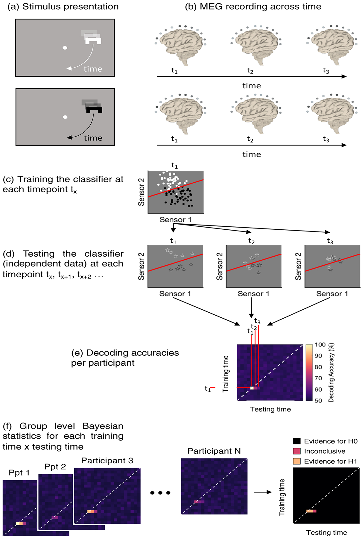
We recorded continuous MEG data while the stimulus was moving on the circular path around the fixation dot (a and b). At each timepoint, we extracted the activation pattern across all MEG channels (c, only two sensors shown for simplicity) and trained a classifier (red line) to distinguish between the different trial types (here black versus white). Then we extracted the sensor activation patterns for independent testing trials (cross-validation) and tested how often the classifier can predict the feature of interest correctly (d). We then used statistical tests to assess at which training- and testing-timepoint combinations the classifier can predict the feature of interest above chance (e). If there is above-chance decoding off the diagonal (white dashed line), information present in the signal at earlier timepoints is reactivated later. (f) shows how the different time-time matrices are combined in order to test for above-chance classification statistically.

We used the CoSMoMVPA toolbox (Oosterhof et al., 2016) to run the time-resolved multivariate analyses. We extracted patterns of brain activity across all 272 MEG sensors at each timepoint, separately for each participant. To distinguish between activation related to the condition of interest (e.g., stimulus shapes; Figure 2a & b), we trained a regularised linear discriminant analysis (LDA) classifier on all but one block of trials (Figure 2c) and then tested the classifier’s performance on the left-out block (independent data; Figure 2d). Above chance classification accuracy at a certain timepoint indicates that the neural data contains information about the different conditions. We used temporal-generalisation methods (Carlson et al., 2011; King & Dehaene, 2014) to examine whether there are recurrent activation patterns over time, that is, whether an activation pattern observed at one timepoint is observed again at a later timepoint. Generalisation off the diagonal in the temporal-generalisation matrix is driven by overlap in the activation pattern at two different timepoints, and therefore implies that the activation pattern recurred. Temporal-generalisation allows us to examine such potential overlaps in representation over time. For example, the shape representation may be similar when the object is visible and when it is occluded. To test this, we trained the classifier at one timepoint and tested it at all other timepoints in the timeseries. This approach results in time-time decoding matrices in which each cell corresponds to a classification accuracy at a unique training- and testing-timepoint combination (Figure 2e).

We also ran sensor-searchlight analyses (Carlson et al., 2019; Collins et al., 2018; Kaiser et al., 2016) to examine the spatial distribution of observed effects. For this analysis, we ran the same analyses as outlined above across small clusters of 9 MEG sensors and projected these back onto topographical plots. These topographical plots may show whether the effects are primarily driven by specific sensor clusters. For the shape and luminance decoding, we ran the sensor-searchlight for the diagonal of the time-time decoding matrices. For the position decoding, we ran the sensor-searchlight analysis for three testing timepoints which were selected based on the pilot data (80 ms, 120 ms, 160 ms). After training on each of these timepoints, we ran the sensor-searchlight across time for the occlusion and disappearance trials. We did not test any specific hypotheses with regard to the spatial distributions of the effects and therefore did not run any statistical tests on the results. Instead, the sensor-searchlight analyses are shown alongside the timecourse results which are the main focus of this study.

2.5.2.1. Shape representation

Decoding the object shape, we tested whether there is position-independent shape information in the neural signal during occlusion. Furthermore, we used temporal-generalisation methods to test whether the time-course of shape processing during occlusion is similar to shape processing of visible, moving objects.

To test for shape-specific information in the signal, we trained a classifier to distinguish between trials in which Shape 1 was shown from trials in which Shape 2 was shown. Then we tested whether the classifier could predict the shape that was shown for each trial in a set of left-out trials. Above chance decoding indicates that shape information is present in the neural signal, providing insights into the time-course of shape processing of moving objects that are not visible. We used an 18-fold cross-validation for all but two participants (due to excluding one trial for each, we ran those participants with a 17-fold cross-validation). Overall, there were six blocks of 96 trials each. Within each block, each unique trial combination (shape × luminance × starting position × movement direction) repeated three times. We trained the classifier on data from 544 trials, leaving out one set of the unique trials at a time (32 in total). We report the overall shape decoding accuracy as well as the accuracy for different starting positions and movement directions to assess whether shape representations were influenced by position. Above chance decoding accuracy means that there was an abstract shape representation in the signal at a given time.

Running the shape analysis on the occlusion trials allows us to compare shape activations before, during and after occlusion. If, for example, the shape representation evoked by the initial stimulus presentation pre-occlusion is similar to the shape representation post-occlusion, we should see above chance decoding off the diagonal of the temporal-generalisation matrix. That would suggest that there is evidence of recurring information at different timepoints (cf. King & Dehaene, 2014). Similarly, if shape representations are similar when the object is visible and when it is occluded, we should be able to cross-generalise between the timepoints of these different phases of the trial. Alternatively, above chance decoding on the diagonal indicates that a unique shape representation occurs at every phase of the trial. Thus, this analysis allows us to probe directly whether shape information during occlusion is perception-like.

Any shape-specific activation observed during occlusion might be driven by the time period prior to occlusion when the shape was visible. To test for this possibility, we ran the same analysis on the disappearance runs to see whether shape-specific activation in the absence of visual stimulation is unique to occlusion or whether it also occurs when an object disappears.

2.5.2.2. Luminance representation

We also tested whether luminance information is present in the neural signal during occlusion and whether the time-course of luminance processing during occlusion is similar to luminance processing of visible objects in motion. We ran the same analyses as the shape decoding analyses (2.5.2.1) but trained the classifier to distinguish between trials in which dark and light stimuli were shown. We ran this analysis in the same way as the shape decoding analysis with an 18-fold cross validation (17-fold for two participants), relying on the fact that the stimulus characteristics are counterbalanced within each block. In addition to overall decoding accuracy, we reported decoding accuracies for the different starting positions and motion directions. Timepoints with above chance decoding provide evidence for luminance information in the neural signal. This gives us the opportunity to test whether luminance information is present in the neural signal when objects are dynamically occluded. In addition, luminance-specific activations before, during and after occlusion can be compared in the same way as for shape decoding.

Again, to test whether luminance-specific activation during occlusion might be driven by the time period when the stimulus was visible, we ran the same analysis on the disappearance trials. This allows us to test whether luminance-specific activation in the absence of visual stimulation is unique to occlusion or whether it also occurs when an object disappears.

2.5.2.3. Position representation

We examined whether position information is represented in the neural signal during occlusion. The position analyses are not straightforward as the position and time are linked: If we look at trials where the object moved in clockwise and counter-clockwise directions separately, the object can only be in four possible positions at a given time. That means that a time-resolved decoding approach is restricted to a four-way classification problem. For the position analyses outlined below, we trained a classifier to use the MEG data to predict where the stimulus is, given four possible positions at a specific time.

Position within-decoding analysis³

For the position within-decoding analysis, we split the trials by movement direction (clockwise and counter-clockwise) and trained the classifier to distinguish the stimulus position at each timepoint. As there were four starting locations, the stimulus could be in one of four positions at each timepoint. We then ran the analysis in a four-way fashion, distinguishing between all possible positions at every timepoint. Above chance decoding in this analysis indicates that there is information about the quadrant in which the object is at a given time. In addition to decoding accuracies, we report confusion matrices for the diagonal of the time-time matrix, showing the error patterns of the predictions. Given that the occluder is the same colour as the background, above chance position decoding can only be driven by the perceived position of the object at a given timepoint. If we had chosen to make the occluder visible, we would not be able to disentangle whether we are decoding the position of the occluder or the position of the object at a given timepoint.

One drawback of the position within-decoding analysis is that it is susceptible to eye-movement artefacts. Tracking of the moving object or even consistent (micro-)saccades towards the object’s position can have an effect on the MEG signal (Quax et al., 2019). Above chance decoding of object position from the MEG signal could thus be (at least partially) driven by eye movements. Note that this issue is unique to the position decoding analysis, as the different shape and luminance conditions are not likely to cause different patterns of eye-movements. In addition, shape and luminance information were decoded across positions. To examine whether the position decoding effects could be driven by eye movements, we ran a control eye tracking analysis (see section 2.6 below). We also ran a cross-decoding analysis between the unpredictable position streams and the occlusion runs for position information, an analysis in which eye movements have much less potential influence.

Position cross-decoding analysis

For the position cross-decoding analysis, we used the unpredictable position streams to train the classifier to distinguish between brain activation patterns associated with the object being in a given position. We then tested whether the classifier, trained on the unpredictable position data, can reliably predict object position in the occlusion (and disappearance) trials. In the unpredictable position streams, consistent eye movements are unlikely because there was no way for the participant to predict where the stimulus would appear. In addition, eye movements have been shown to affect MEG data ~200ms after lateralised stimulus onset (Quax et al., 2019) which means that the brief presentation durations used in the unpredictable position streams (33 ms + 100 ms inter-stimulus-interval) are unlikely to lead to consistent eye movements.

As there is no predictable motion in these trials, the temporal dynamics of position information might be different in comparison to the occlusion trials. It is, for example, possible that position information is accessed earlier when an object follows a predictable motion path in comparison to when it appears in random positions. To capture these potentially different dynamics, we ran the position decoding analysis across time (temporal-generalisation). Since the object is moving in the occlusion trials, we were not able to assign a single position label to the entire trial but rather we broke each occlusion trial up into single presentation durations (33.3 ms each). We then merged the classification accuracies in each of these small epochs back together to cover the entire presentation duration of a single trial (−200 – 2000 ms). Note that at each timepoint in the occlusion trial, the stimulus can only be in one of four possible positions (chance decoding is 25%). To capture the error patterns, we report the confusion matrices using three different training timepoints (80 ms, 120 ms, and 160 ms) which were chosen based on the pilot data.

Both the position within-decoding and cross-decoding analyses provide novel information about the time-course of position processing for moving objects that are going through brief periods of occlusion. In addition, it is possible that the time-course of position processing is influenced by predictability. The position decoding analyses allow us to test this by comparing phases of the trial where stimulus position is predictable (i.e., post-occlusion) and when it is unpredictable (i.e., initial appearance of the stimulus). In addition, we are able to differentiate between position-specific activation when the object is invisible due to occlusion (i.e., the stimulus is out of sight) versus disappearance (i.e., the stimulus ceased to exist).

The key difference between the position within- and cross-decoding analyses outlined above is that in the within-decoding analysis, the classifier is trained and tested on the occlusion/disappearance trials, while in the cross-decoding analysis, the classifier is trained on the unpredictable position streams and tested on the occlusion/disappearance trials. The cross-decoding analysis aims to identify position information in the signal that is independent of motion or predictability and hence unlikely to be driven by eye movements. However, it is possible that the neural signature for stimuli with an immediate onset is very different from smoothly moving and predictable stimuli, making cross-generalisation between these two different trial types difficult. Therefore, both of these analyses are valuable in different ways and should be interpreted together.

2.6. Eye tracking analyses

Eye movements are a potential confound for the position within-decoding analysis. To test for an influence of eye movements, we ran the same position within-decoding analysis used for the MEG data on our eye tracking data. We trained the classifier to distinguish between the different positions at each timepoint but this time using only the X- and Y-coordinates of the eye tracking data. We used mutual information analyses (Quax et al., 2019) to examine at which timepoints eye movements are a potential problem for our MEG analyses. For the mutual information analysis, we determined which positions the classifier predicts at each timepoint in the occlusion trials when it is trained on the MEG data and the eye tracking data, and then tested whether there is mutual information between the eye tracking and the MEG data. Above-chance decoding at timepoints with mutual information have to be interpreted with caution.

2.7. Statistical inference

We used Bayes Factors (Dienes, 2011; Good, 1979; Kass & Raftery, 1995; Morey et al., 2016; Rouder et al., 2009; Wagenmakers, 2007) to determine the evidence for above-chance decoding (i.e., alternative hypothesis) and for chance decoding (i.e., null hypothesis) at every timepoint. We used a hybrid one-sided Bayesian test (Morey & Rouder, 2011), testing against a point-null of effect size 0 (chance decoding) that deems small positive effect sizes as irrelevant. We used a half-Cauchy prior for the alternative hypothesis with a default, medium width of $r=\frac{\sqrt{2}}{2}=0.707$. We defined the standardized effect sizes to occur under the alternative to be in a range between 0.5 to infinity, capturing directional (above chance) medium sized effects (Morey & Rouder, 2011). Additionally, we ran a robustness check, testing whether the observed effects remain when we choose a wide (r = 1) and ultrawide (r = √2 = 1.414) scale for the prior width. Our chosen prior distribution assumes that a wide range of effect sizes is possible but that medium effect sizes are more likely (Keysers et al., 2020). We used the Bayes Factor R package to calculate the BFs (Morey et al., 2015) implemented within Matlab (Teichmann, Moerel, et al., 2021).

Bayes Factors (BFs) that are smaller than 1 indicate that there is more evidence for the null hypothesis (chance and below-chance decoding) in the data than for the alternative hypothesis (above chance decoding), whereas BFs that are larger than 1 indicate that there is more evidence for the alternative hypothesis than for the null hypothesis (Dienes, 2011). Here, we used the BF cut-off of 6 and interpret this as substantial evidence for above chance decoding (Wetzels et al., 2011). BF smaller than 1/6 will be used as evidence for the null hypothesis which indicates that decoding is around chance.

In addition to decoding accuracies, we also looked at decoding latencies. To do this, we examined the time period of peak decoding by sub-selecting a different set of decoding timeseries from the participants 10,000 times and then calculated the 95% confidence interval for the peak latency. These bootstrapped peak confidence intervals for each phase of the trial (pre-occlusion, occlusion, and post-occlusion) give the opportunity to directly compare the time at which we can best decoding shape, luminance, and position.

2.8. Transparency and openness

The raw and preprocessed data for this study can be found on OpenNeuro (http://doi.org/doi:10.18112/openneuro.ds004011.v1.0.1). All analysis codes were uploaded to OSF (https://osf.io/hc25w/). The accepted stage 1 submission for this registered report can be found on OSF (https://osf.io/tp2ad).

2.9. Changes to the pre-registered study

1. We used a different MEG system for the pilot and for the main experiment. We made the following changes to the planned pre-processing of the MEG experiment data to match pre-processing as closely as possible to the pilot. The MEG system that was used for the pilot study automatically applied an online low-pass filter at 200 Hz. We applied a 200 Hz low-pass filter to the experiment data to keep this consistent with the pilot dataset. The pilot MEG system also applied an online high-pass filter. However, high-pass filtering can distort results in decoding studies (van Driel et al., 2021). To match the MEG data as closely as possible between the experiment and pilot, without relying on high-pass filtering, we used robust linear detrending with a baseline correction (see section 2.5.1).

2. We encountered the following problems during data collection. First, we were not able to use continuous head motion tracking due to broken hardware. Instead, we monitored participants closely and recorded coil positions after every run (see section 2.1). In addition, there were two instances of very brief (<100ms) MEG signal dropouts. We removed the two affected trials from the data analysis.

3. We made the following changes for clarity. First, we changed the labelling of the selected time window. In the pilot data, the stimulus did not emerge gradually so 0 ms referred to the trial start as well as the time that the stimulus first became visible. In the main experiment, we initially proposed to set 0 ms to the trial start. However, because the stimulus emerged gradually from behind an occluder, the object then became visible at ~200 ms. To match the convention of referring to the stimulus onset as 0 ms, we now refer to 0 ms when the stimulus first becomes visible. Note that the epoch is the same as proposed, only the label of 0 ms has changed for clarity (see section 2.5.1). In addition, we renamed the “quadrant analysis” to “position within-decoding”, to better clarify the difference with the “position cross-decoding” analysis (see section 2.5.2.3). Finally, we removed a sentence about regression analysis that was in the stage 1 manuscript by mistake.

4. In response to the reviewers’ comments, we added an eye tracking analysis using the X- and Y-coordinates from the unpredictable position runs to predict the responses during the occlusion and disappearance runs. This analysis was used to examine the potential effect eye movements could have on the position cross-decoding analysis.

3. Results

In this study, we used MVPA on MEG data to investigate whether object representations during occlusion are rich and perception-like or abstract. Our results show evidence for object shape, luminance, and position information when the object was visible. However, evidence for luminance and shape information was weak during occlusion, and position information was only maintained for the initial occlusion period. We outline the results for each analysis in detail below. As outlined in the methods section, we used Bayes Factors to statistically assess the decoding results. While we used three different common prior widths (medium, wide, ultrawide) to assess for robustness of our results, we here report only the BFs for the default, medium width prior, as the different prior widths did not affect the results. Bayes Factors for all analyses and prior widths can be found on OSF.

3.1. Shape representation

We examined the time-course of position-independent shape information before, during, and after occlusion (see Figure 3A, row 1). There was position-independent shape information before and after occlusion – when the object was visible. During occlusion, there was information about the object shape for some timepoints, but most timepoints showed evidence for the null hypothesis (i.e., chance decoding of shape). To assess whether shape representations were influenced by position, we determined the shape decoding separately for the different positions (i.e., different start positions and movement directions), and then averaged the decoding accuracies across the different positions. The results were similar to the position-independent shape decoding: There was some shape information before and after occlusion (see Figure 3A, row 2). Some timepoints showed evidence for position-dependent shape decoding during occlusion, although most timepoints showed evidence for the null hypothesis (i.e., chance decoding). The sensor searchlight analysis indicated that the shape decoding during the visible periods is mostly driven by posterior sensors.

Figure 3. Shape decoding results for the occlusion (A) and disappearance (B) conditions.

A) Shape decoding for the occlusion condition. Black dashed lines are used throughout to indicate the timepoints when the object is visible or invisible, with the object being partially visible in between these times. Row 1 shows the time-series of shape decoding along the diagonal (i.e., for the same training and test timepoint). Theoretical chance is 50% decoding accuracy. The black line shows the mean decoding accuracy over time (temporally smoothed with a kernel of 5 timepoints for plotting clarity only). Shaded error bars around the black line indicate the standard error of the mean. We calculated the bootstrapped peak times separately for the time windows before occlusion, during occlusion, and after occlusion. The 95% confidence intervals of the bootstrapped decoding peak times are the grey bars displayed below the decoding accuracies. We obtained time-varying topographies from the channel-searchlight analysis, and averaged across all timepoints before occlusion, during occlusion, and after occlusion. Bayes factors (BFs) over time are shown below the timecourse. BFs are plotted on a logarithmic scale for the decoding for each combination of training and test timepoints displayed in row 1. BFs supporting the alternative hypothesis are shown in red and BFs supporting the null hypothesis are shown in blue. Row 2 shows the position-dependent shape decoding over time for the same training and test timepoint, with the BFs shown below the timeseries. Plotting conventions are the same as in Row 1. Rows 3 and 4 show the results of the temporal-generalisation analysis. We trained a linear classifier on all timepoints of the occlusion trials in the training set and tested the classifier on all timepoints of separate occlusion trials in the test set. The colours represent the decoding accuracy for each combination of training and test timepoints, with the green colours indicating above chance decoding. The BF plotting conventions in Row 4 are the same as in rows 1 and 2. Together, rows 3 and 4 suggest that there is some evidence for shape information when the object is visible. There is only limited evidence for shape information in the signal when the object is occluded. B) The same analyses as in A are repeated for the disappearance condition. Note the time-course for this task is shorter, as the stimulus does not re-appear.

We used temporal-generalisation methods to determine whether the position-independent shape information was similar before, during and after occlusion (Figure 3A, row 3 shows decoding accuracies and row 4 shows Bayes Factors). The results show off-diagonal shape generalisation in decoding for the object before and after occlusion. This shows that the neural pattern evoked by the shape of the object is similar for these different points in time. The shape decoding during occlusion did not generalise to decoding before and after occlusion, suggesting the neural pattern during occlusion was different to that evoked by the shapes during perception.

Feature representations during occlusion could be driven by perpetuation of feature-specific activation during the time prior to occlusion, which would not be unique to occlusion. Our disappearance condition provides a control to test for occlusion-specific effects. We therefore repeated the same analyses described above for the disappearance condition. Overall, the results were very similar for the disappearance and occlusion condition. There was position-independent shape information before disappearance and weak evidence for shape decoding for some timepoints after the shape had disappeared, but most timepoints after disappearance supported the null hypothesis (see Figure 3B, row 1). We examined evidence of position-dependent shape information by determining shape decoding separately for the different positions and found that there was position-dependent shape information before the stimulus disappeared (see Figure 3A, row 2). In addition, there was evidence for position-dependent shape information after the stimulus disappeared for some timepoints. The temporal-generalisation data showed that visible position-independent shape information did not generalise to the time after the stimulus disappeared (see Figure 3B, rows 3 and 4).

3.2. Luminance representation

In addition to shape information, we examined whether there was luminance information in the signal. Overall, the signal for luminance decoding was stronger than that of shape (see Figure 4). We found evidence for position-independent and position-dependent luminance information before and after occlusion which was mostly driven by posterior sensors (see Figure 4, rows 1 and 2). In addition, there was some evidence for above chance position-independent luminance decoding during occlusion. In contrast, position-dependent luminance decoding was at chance during occlusion which may be due to the fact that fewer trials were used to train the position-dependent luminance classifier (see methods). The temporal-generalisation analyses showed that the position-independent shape information was similar before and after occlusion as indicated by off-diagonal generalisation of luminance decoding (Figure 4A, panel rows 3 and 4). However, the neural pattern evoked by the object luminance when the object was occluded did not generalise to when it was visible, indicating that there is a difference in luminance representation when the object is visible and invisible.

Figure 4. Luminance decoding results for the occlusion (A) and disappearance (B) conditions.

All plotting conventions are the same as in Figure 3. A) Luminance decoding for the occlusion condition. Row 1 shows the position-independent luminance decoding on the diagonal. Row 2 shows the position-dependent luminance decoding over time. Row 3 shows the temporal-generalisation for position-independent luminance decoding, and Row 4 shows the corresponding Bayes factors on a logarithmic scale. B) The same analyses were repeated for the disappearance condition.

We investigated whether luminance decoding during occlusion could be driven by lingering activation from the time prior to occlusion by repeating the analyses for the disappearance condition. We found evidence for luminance decoding when the object was visible (see Figure 4B, rows 1 and 2). In addition, there was evidence for luminance decoding after the object had disappeared, suggesting the luminance decoding found during occlusion might not be driven by the occlusion process, but rather by general offset effects. The temporal-generalisation showed no evidence for generalisation from when the stimulus was visible to when it was invisible (see Figure 4B, rows 3 and 4).

3.3. Position representation

3.3.1. Position within-decoding analysis

To investigate whether the position of the object is represented before, during, and after occlusion, we ran the position within-decoding analysis. We split the data by movement direction for this analysis, which means the object could be in one of four possible positions at any given time. For the occlusion task, there was information about the quadrant in the signal when the object was visible and invisible (Figure 5A, row 1). A sensor searchlight showed that the position decoding was mostly driven by posterior sensors (Figure 5A, row 1). Decoding accuracies were highest along the diagonal and during the visible period (before and after occlusion), but there was a clear spread to neighbouring timepoints (Figure 5A, rows 2 and 3). Position information did not generalise between the time before and after occlusion and showed below chance decoding, which would be expected because the object was always in a different quadrant before occlusion in comparison to after occlusion. We furthermore examined the classifier errors which could provide insight into which position is represented at a given time. Focusing on the diagonal of the temporal-generalisation matrix, we plotted the percentage of predictions for each quadrant at each timepoint. When the object was visible (before and after occlusion), the classifier was most likely to predict the correct quadrant and least likely to predict the opposite quadrant. During occlusion, this pattern of predictions remained (Figure 5A, row 4).

Figure 5. Position within-decoding results for the occlusion (A) and disappearance (B) condition.

All plotting conventions are the same as in Figure 3. A) Position decoding for the occlusion task. Row 1 shows time-series decoding along the diagonal along with BFs and time-varying topographies from the channel-searchlight analysis. We trained a linear classifier to distinguish between the object position in one of four possible quadrants. Therefore, theoretical chance is at 25%. Bootstrapped peak decoding time 95% confidence intervals are shown as grey bars above the topographies. Row 2 shows the temporal-generalisation for position decoding. The colours represent the decoding accuracy per combination of training and test timepoints. Green colours indicate above chance decoding. Row 3 shows the corresponding Bayes factors on a logarithmic scale, with BFs supporting the alternative hypothesis shown in red and BFs supporting the null hypothesis shown in blue. Row 4 shows the classifier predictions for the diagonal (i.e., same training and test timepoint). The classifier can predict the correct quadrant, previous or next quadrant, or the opposite quadrant. The colours show how often the classifier predicted each quadrant (theoretical chance is 25%). B) Same analyses described in A but for the disappearance condition.

We repeated these analyses for the disappearance condition to ascertain whether the position decoding during occlusion could be driven by lingering activation prior to occlusion. Overall, the results for the disappearance condition looked very similar to the occlusion condition. We found evidence for position decoding when the object was visible and after it had disappeared (see Figure 5B, row 1). The sensor searchlight showed that the posterior sensors contributed the most to the position decoding (Figure 5B, row 1). The decoding was highest along the diagonal, but spread to neighbouring timepoints (see Figure 5B, rows 2 and 3), mirroring the results found in the occlusion analysis. The diagonal predictions for the disappearance task showed that the classifier was most likely to predict the correct quadrant, and least likely to predict the opposite quadrant, both before and after the disappearance (Figure 5B, row 4). Overall, the high similarity between the position effects in the occlusion and disappearance conditions suggests that position information during invisible periods is not specific to occlusion. However, the disappearance condition may not be a reliable control for occlusion, as participants may be primed to see the object to re-appear after viewing many occlusion trials. In addition, the gradual nature of disappearance may strengthen the intuition that the object may re-appear. We further explore these caveats in the discussion (section 4.3).

3.3.2. Position cross-decoding analysis

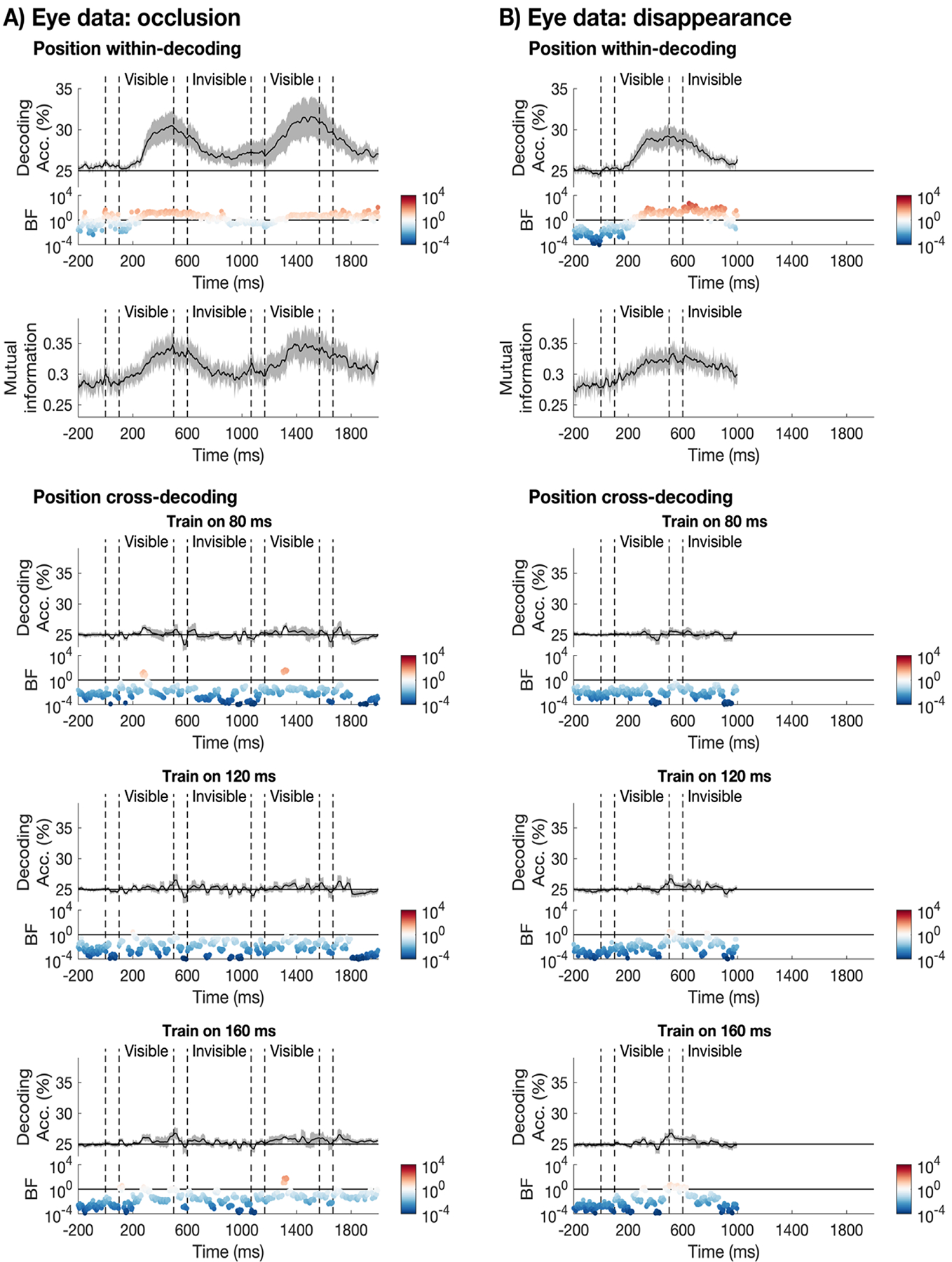
The position within-decoding results described above could be driven, at least in part, by eye movements. We therefore used a position cross-decoding analysis, where we trained the classifier on the unpredictable position streams to distinguish between possible object positions and tested the classifier on object position in the occlusion and disappearance trials. As stimulus location was unpredictable for the training dataset, any consistent eye movements in the test set cannot influence the decoding success. We ran this analysis separately for the two movement directions, which means that the object can be in four possible positions at a given time as there were four different starting positions. For the unpredictable position stream, the objects appeared in one of all 64 possible positions. To train the classifier at each timepoint, we selected unpredictable position trials where the object was in one of the four possible positions to match the test set. Thus, theoretical chance was at 25% as the classifier was trained and tested to distinguish four different positions at each timepoint. The results for the occlusion condition showed that there was information about the position when the object was visible (before and after occlusion; see Figure 6A, rows 1 and 2). There was evidence for position decoding when the object was occluded in the first 200 ms of the occlusion period, after which position decoding was at chance.

Figure 6. Position cross-decoding results for the occlusion (A) and disappearance (B) tasks.

All plotting conventions are the same as in Figure 3. A) Position cross-decoding for the occlusion task. Row 1 shows the temporal-generalisation for position decoding. We trained the classifier on unpredictable object position data and tested the classifier on object position in the occlusion trials. Theoretical chance is at 25%. Green colours indicate above chance decoding. Row 2 shows the corresponding Bayes factors on a logarithmic scale. Horizontal coloured dashed lines are used to indicate the training times of 80 ms (orange), 120 ms (red), and 160 ms (blue), for which we analysed the classifier predictions (see row 3–5). Row 3 shows the classifier predictions for a classifier trained on the unpredictable object position data at 80ms after stimulus onset. The colours show how often the classifier predicted each position (correct quadrant, previous or next quadrant, or the opposite quadrant). Theoretical chance is at 25%. Panel 4 shows the classifier predictions for a classifier trained at 120ms after stimulus onset, and panel 5 for a classifier trained at 160ms after stimulus onset. B) Same analyses described in A but for the disappearance condition.

To gain insight into the predictions of the classifier, we analysed the classifier predictions for classifiers trained at three specific timepoints (80 ms, 120 ms, and 160 ms) chosen based on the pilot data (see supplementary information). No clear patterns were apparent for the classifier predictions trained on data from 80 ms after stimulus onset (Figure 6A, row 3). However, an interesting pattern emerged for classifiers trained at 120 ms (Figure 6A, row 4) and 160 ms (Figure 6A, row 5) after stimulus onset. When the object was visible (before and after occlusion), the classifier was most likely to predict the correct quadrant and least likely to predict the opposite quadrant. However, after ~200 ms of occlusion, the classifier was most likely to predict the next quadrant. This suggests that instead of tracking the motion during occlusion, the position representation jumps ahead to the location where the object is expected to reappear.

To determine whether the position coding during occlusion could be driven by the time prior to occlusion, we repeated the analysis for the disappearance task. Overall, the results for the disappearance condition were very similar to the results of the occlusion condition. There was position coding when the object was visible and briefly after the disappearance (Figure 6B, rows 1 and 2), similar to the object coding during occlusion. The predictions showed no clear pattern for the classifier trained at 80 ms after stimulus onset (Figure 6B, row 3). However, the predictions for the classifiers trained at 120 ms (Figure 6B, row 4) and 160 ms (Figure 6B, row 5) showed a similar pattern to that found for the occlusion condition. When the object was visible, the classifier was most likely to predict the correct quadrant and least likely to predict the opposite quadrant. After the object had disappeared, the most likely prediction jumped from the correct quadrant to the next quadrant, where the object reappeared in the occlusion trials. This suggests implicit predictions of where the object reappears after occlusion might have persisted into the disappearance task, where the object did not reappear. We discuss this possibility in more detail in the discussion.

3.4. Eye tracking analyses

To test whether eye-movements were a potential confound for the quadrant position decoding analysis, we ran the same analysis on the eye tracking data. We trained the classifier to distinguish between the different positions at each timepoint using the X- and Y-coordinates of the eye tracking data. The results showed above chance decoding when the object was visible in the occlusion task (Figure 7A, row 1). In addition, there was evidence for above chance position decoding during occlusion. We also assessed whether there was mutual information between the eye tracking and the MEG data (Quax et al., 2019). The mutual information is shown in row 2 of Figure 7A, with mutual information values of zero indicating that the MEG signal and eye position are independent, and larger values indicating a greater relationship between them. There was mutual information between the eye tracking and the MEG data for the occlusion task. Running the position cross-decoding analysis on the X- and Y-coordinates of the eye tracking data showed that there is no reliable information about the object position in the unpredictable position eye tracking data (Figure 7A, rows 3–5). This highlights that the position-cross decoding analysis is unlikely to be biased by eye movements.

Figure 7. Eye tracking analyses.

All plotting conventions are the same as in Figure 3. A) Eye tracking analyses for the occlusion task. Row 1 shows the position within-decoding for the diagonal (i.e., training and testing on the same timepoint). Shaded error bars indicate the standard error of the mean. The mean decoding accuracy (black line) was temporally smoothed with a kernel of 5 timepoints for plotting clarity only. Bayes factors are shown on a logarithmic scale below the plot. BFs supporting the alternative hypothesis are shown in red and BFs supporting the null hypothesis are shown in blue. Row 2 shows the mutual information between the eye tracking and the MEG data. Plotting conventions are the same as in Panel 1. Row 3–5 show the position cross-decoding analysis based on the eye tracking data for the selected training timepoints (80 ms, 120 ms, 160 ms). The corresponding Bayes Factors are shown below each plot. B) Same analyses but for the disappearance condition.

We found similar results for the disappearance condition, there was evidence for above chance quadrant decoding using the eye tracking data, both when the object was visible and after it had disappeared (Figure 7B, row 1). In addition, there was mutual information between the eye tracking and the MEG data for the disappearance condition (Figure 7B, row 2). For the position cross-decoding analysis, we did not find reliable position information in the eye tracking data. Together, these results suggests that eye movements could have contributed to the position within-decoding analysis but not to the position cross-decoding. We therefore must interpret the results from the position within-decoding analysis with caution. We further consider the implications of this in the discussion.

3. Discussion

When an object briefly moves out of sight due to occlusion, we often have the impression that the object persists. The aim of the current study was to examine the nature of object representations during such dynamic occlusion events. Specifically, we tested whether the representation of objects during occlusion is feature-rich and perception-like or more abstract. Using sensor-based MEG classification analyses, when the object was visible, we could decode information from the neural signal about object shape, luminance, and position, albeit with stronger evidence for position than shape or luminance. During occlusion, position information was maintained in the initial period for ~200ms, but evidence for luminance and shape representation was weak to non-existent. This challenges the notion that there is a continued, feature-rich representation of object properties during periods of occlusion (cf. Gibson et al., 1969).

4.1. Maintained and updated position representations during occlusion

Resolving motion over periods of occlusion requires an integration of information over space and time. We showed that there is information about object position and object features in the neural signal while the object is visible before and after occlusion. Previous work has shown that the integration of visible motion trajectories before and after occlusion is so strong that slight inconsistencies between object features before and after occlusion are overruled if the timing and position of the object re-appearing is consistent (e.g., Burke, 1952; Carey & Xu, 2001; Flombaum et al., 2009; Yi et al., 2008). For example, when a differently coloured object reappears after occlusion at the right time and place, we tend to perceive the reappearing object to be the same object as that seen prior to occlusion just with a changed feature. This indicates that we value spatiotemporal consistency higher than featural consistency, despite the fact natural objects typically do not change colour or shape. Our results show that position information is present in the signal before and after occlusion, presumably allowing for the integration between visible motion trajectories bridging the occlusion period.

During occlusion, position information was maintained to a certain degree but after an initial period, predictions about the next visible position dominated. Previous work on visible motion has shown that predictions of motion trajectories are always taking place (Blom et al., 2020), potentially to account for the delay between a visual event happening in the external world and our internal perception of that event (Hogendoorn, 2021). Predicting or extrapolating motion trajectories ahead of time has been shown to extend into perceptual gaps such as eyeblinks (Maus et al., 2020) and the retinal blind spot (Maus & Nijhawan, 2008; Shi & Nijhawan, 2012). Similarly, our data show that position information is represented in the initial occlusion period, indicating that motion information is extrapolated into the perceptual gap caused by occlusion. After this initial period of occlusion, we found no reliable position information when using a cross-generalisation approach, training the classifier on trials from the unpredictable position stream where stimuli were visible. Looking at the predictions in the cases of misclassification showed that the later timepoints during occlusion carry information about the location where the object will re-appear after occlusion. Thus, these results show that there is accurate motion extrapolation into the initial period of occlusion with an abrupt change in prediction to the leading quadrant where the object is expected to become visible again.

In contrast to the cross-classification approach, there was evidence for position information throughout the occlusion period when training and testing the classifier on the occlusion trials. One possible explanation for this difference is that eye movements contributed to the above-chance classification in this within-classification position analysis. The mutual information analysis indeed showed that there was mutual information between the MEG data and the eye tracking data. However, it is also possible the mutual information between the MEG data and eye data reflected the expectation of the position of the occluded object. In particular, the position cross decoding analysis, which is highly unlikely to be influenced by eye movements, shows that there are strong predictions about the object’s reappearance position post-occlusion. Thus, if both the eye tracking and MEG data carry information about the reappearance position, the mutual information analysis would pick on this commonality. In line with this interpretation, we found that posterior sensors are the main contributor to the above-chance classification, which is not consistent with eye movements alone driving the above-chance classification (we would expect frontal sensors to be primarily recording eye movement signals). Another possible explanation for the difference between the position within-decoding and position cross-decoding results is that the signal evoked by visible motion is different to that of invisible or imagined motion. Previous work has shown that imagined motion evokes a temporally diffuse signal while visible motion is temporally more aligned (Robinson et al., 2021). Thus, it seems likely that representations during the later stages of occlusion are maintained in a different way, making it challenging to pick up on meaningful information with a cross-classification approach.

4.2. Limited evidence for object identity feature representation during occlusion

In addition to examining position information, we investigated the representation of object identity features (luminance and shape) and found little to no evidence that these features are maintained during occlusion. When the object was visible, there was some evidence for shape and luminance information in the neural signal, however, evidence was weaker in comparison to position information. Additionally, we were able to cross-generalise from pre-occlusion to post-occlusion timepoints highlighting that the position-independent representations of object identity before and after occlusion are similar. During occlusion, object feature information was limited and if present, temporally diffuse. We could not successfully cross-generalise from the times when the stimulus was visible to the times when the object was occluded, which could mean that the representation of object identity through occlusion is not perception-like. However, we must be careful with this interpretation as the evidence for object feature information was relatively weak even during the visible period, making the lack of effects during occlusion difficult to interpret. Visible stimuli usually evoke stronger and more temporally-aligned signal than imagined or internally-generated signals (e.g., Robinson et al., 2021; Teichmann et al., 2019; Teichmann, Grootswagers, et al., 2021). Here, however, the evidence for shape and luminance representation for visible moving stimuli in the periphery were already weak. A likely explanation for unreliable representations of visible stimuli in the periphery is cortical magnification. Specifically, we would expect to see weaker signals in response to stimuli presented in the periphery in comparison to stimuli presented at the fovea, as the receptive field size increases. A stimulus presented in the periphery engages a smaller cortical portion which, in turn, means we would need a finer scale to record distinguishable patterns of activity for peripheral stimulus presentation versus foveal presentation. It is also possible that the representation of object features during occlusion depends on task demands. In our initial pilot (see supplementary materials), we found that participants were able to report whether an object that reappeared after occlusion was the same or different. This indicates that information about the object identity must be retained to some extent. In fact, the data collected while participants focus on the object identity feature show above-chance decoding during occlusion for object shape. In the current experiment, we focussed on the “automatic” aspect of occlusion and not attention or working memory. Therefore, we used a task that did not require maintenance of the stimulus features. Given the results, it seems that shape and luminance are not automatically maintained in a perception-like fashion during occlusion. A possible explanation for the lack of evidence is that there is no need to automatically maintain all features of an object while it is out of sight, as identity features tend to remain unchanged. Building on the idea that visual perception is serially dependent (cf. Fischer & Whitney, 2014), it may be that the representation of identity features during occlusion is paused and then biased towards the last visible information prior to the gap. In contrast to object identity features, position information changes through the period of occlusion, thus updating information is required to make accurate predictions.

4.3. Caveats and future directions

All effects we observed were highly similar for the occlusion and the disappearance condition. While this could challenge the notion that “going out of sight” is fundamentally different from “ceasing to exist” (Gibson et al., 1969), the disappearance condition may be limited in serving as a reliable control for occlusion. First and foremost, it seems likely that participants were primed to expect the object to reappear, as it did in half of the experiment. Examining the position predictions right after the disappearance supports this idea, showing that there is an abrupt change from motion extrapolation to an expectancy of the object to reappear in the following quadrant. Second, the gradual nature of disappearance was chosen to match the occlusion and disappearance conditions closely, as we know that visual offset effects can be strong (Carlson et al., 2011). However, gradual offsets make it more likely that an object continues to exist while sudden offsets overwrite extrapolated motion trajectories (Blom et al., 2020; Hogendoorn, 2020; Maus & Nijhawan, 2006, 2009; Nijhawan, 2002, 2008). Thus, it is possible that the controlling the gradual nature artificially created the similarity between occlusion and disappearance conditions. Lastly, it is possible that the difference between shrinking and gradually moving behind an occluder was perceptually not large enough. It was important for participants to fixate so that potential eye movement effects did not overpower small neural signals. However, fixating also meant that the object appeared in the periphery, which might have made the difference between occlusion versus brief period of shrinking for disappearance less obvious. Thus, in the future it would be useful to contrast gradual occlusion events with sudden offsets.

In the current experiment, we asked participants to maintain fixation throughout the task. However, fixating centrally while an object moves in the periphery does not reflect natural vision. In everyday life, eye movements may be critical to fill in lacking visual information during occlusion. Future work could investigate to what extent eye movements contribute to the maintenance of occluded visual information. Another potential avenue for future work could be to investigate object representations through different types of perceptual gaps. For example, internally-driven events such as eyeblinks and saccades occur frequently and also interrupt visual information reaching the brain (Teichmann, Edwards, et al., 2021). It would be interesting to examine whether dynamic visual input is resolved in the same way through these types of perceptual gaps.

4.4. Conclusion

Overall, our findings suggest that information that changes over the occlusion period, such as position information, is maintained and updated to some extent before prediction for the next visual event occurs. For object features that do not typically change, such as luminance and shape, there is less evidence for automatic maintenance through occlusion. In conclusion, these results challenge the idea that the representation of visual information during periods of occlusion is rich and perception-like and contribute to understanding how the visual system bridges perceptual gaps.

References

- Aguiar A, & Baillargeon R (1999). 2.5-month-old infants’ reasoning about when objects should and should not be occluded. Cognitive Psychology, 39(2), 116–157. [DOI] [PubMed] [Google Scholar]
- Assad JA, & Maunsell JH (1995). Neuronal correlates of inferred motion in primate posterior parietal cortex. Nature, 373(6514), 518–521. [DOI] [PubMed] [Google Scholar]
- Baillargeon R (1993). The object concept revisited: New directions in the investigation of infants’ physical knowledge. Visual Perception and Cognition in Infancy, 23, 265–315. [Google Scholar]
- Baillargeon R (2008). Innate ideas revisited: For a principle of persistence in infants’ physical reasoning. Perspectives on Psychological Science. [DOI] [PMC free article] [PubMed] [Google Scholar]
- Baker C, Keysers C, Jellema T, Wicker B, & Perrett D (2001). Neuronal representation of disappearing and hidden objects in temporal cortex of the macaque. Experimental Brain Research, 140(3), 375–381. [DOI] [PubMed] [Google Scholar]
- Barborica A, & Ferrera VP (2003). Estimating invisible target speed from neuronal activity in monkey frontal eye field. Nature Neuroscience, 6(1), 66–74. [DOI] [PubMed] [Google Scholar]
- Blom T, Feuerriegel D, Johnson P, Bode S, & Hogendoorn H (2020). Predictions drive neural representations of visual events ahead of incoming sensory information. Proceedings of the National Academy of Sciences, 117(13), 7510–7515. [DOI] [PMC free article] [PubMed] [Google Scholar]
- Burke L (1952). On the tunnel effect. Quarterly Journal of Experimental Psychology, 4(3), 121–138. [Google Scholar]
- Carey S, & Xu F (2001). Infants’ knowledge of objects: Beyond object files and object tracking. Cognition, 80(1–2), 179–213. [DOI] [PubMed] [Google Scholar]
- Carlson TA, Grootswagers T, & Robinson AK (2019). An introduction to time-resolved decoding analysis for M/EEG. ArXiv Preprint ArXiv:1905.04820. [Google Scholar]
- Carlson TA, Hogendoorn H, Kanai R, Mesik J, & Turret J (2011). High temporal resolution decoding of object position and category. Journal of Vision, 11(10), 9–9. [DOI] [PubMed] [Google Scholar]
- Cohen MA, Botch TL, & Robertson CE (2020). The limits of color awareness during active, real-world vision. Proceedings of the National Academy of Sciences. [DOI] [PMC free article] [PubMed] [Google Scholar]
- Collins E, Robinson AK, & Behrmann M (2018). Distinct neural processes for the perception of familiar versus unfamiliar faces along the visual hierarchy revealed by EEG. NeuroImage, 181, 120–131. [DOI] [PMC free article] [PubMed] [Google Scholar]
- Dienes Z (2011). Bayesian versus orthodox statistics: Which side are you on? Perspectives on Psychological Science, 6(3), 274–290. [DOI] [PubMed] [Google Scholar]
- Erlikhman G, & Caplovitz GP (2017). Decoding information about dynamically occluded objects in visual cortex. NeuroImage, 146, 778–788. [DOI] [PMC free article] [PubMed] [Google Scholar]
- Eskandar EN, & Assad JA (1999). Dissociation of visual, motor and predictive signals in parietal cortex during visual guidance. Nature Neuroscience, 2(1), 88–93. [DOI] [PubMed] [Google Scholar]
- Fischer J, & Whitney D (2014). Serial dependence in visual perception. Nature Neuroscience, 17(5), 738–743. [DOI] [PMC free article] [PubMed] [Google Scholar]
- Flombaum JI, Kundey SM, Santos LR, & Scholl BJ (2004). Dynamic object individuation in rhesus macaques: A study of the tunnel effect. Psychological Science, 15(12), 795–800. [DOI] [PubMed] [Google Scholar]
- Flombaum JI, & Scholl BJ (2006). A temporal same-object advantage in the tunnel effect: Facilitated change detection for persisting objects. Journal of Experimental Psychology: Human Perception and Performance, 32(4), 840. [DOI] [PubMed] [Google Scholar]
- Flombaum JI, Scholl BJ, & Santos LR (2009). Spatiotemporal priority as a fundamental principle of object persistence. The Origins of Object Knowledge, 135–164. [Google Scholar]
- Gibson JJ, Kaplan GA, Reynolds HN, & Wheeler K (1969). The change from visible to invisible. Perception & Psychophysics, 5(2), 113–116. [Google Scholar]
- Good IJ (1979). Studies in the history of probability and statistics. XXXVII AM Turing’s statistical work in World War II. Biometrika, 393–396. [Google Scholar]
- Grill-Spector K, Kushnir T, Edelman S, Avidan G, Itzchak Y, & Malach R (1999). Differential processing of objects under various viewing conditions in the human lateral occipital complex. Neuron, 24(1), 187–203. [DOI] [PubMed] [Google Scholar]
- Grootswagers T, Robinson AK, & Carlson TA (2019). The representational dynamics of visual objects in rapid serial visual processing streams. NeuroImage, 188, 668–679. [DOI] [PubMed] [Google Scholar]
- Grootswagers T, Robinson AK, Shatek SM, & Carlson TA (2019). Untangling featural and conceptual object representations. BioRxiv, 607499. 10.1101/607499 [DOI] [PubMed] [Google Scholar]
- Grootswagers T, Wardle SG, & Carlson TA (2017). Decoding Dynamic Brain Patterns from Evoked Responses: A Tutorial on Multivariate Pattern Analysis Applied to Time Series Neuroimaging Data. Journal of Cognitive Neuroscience, 29(4), 677–697. 10.1162/jocn_a_01068 [DOI] [PubMed] [Google Scholar]
- Halgren E, Dale AM, Sereno MI, Tootell RB, Marinkovic K, & Rosen BR (1999). Location of human face-selective cortex with respect to retinotopic areas. Human Brain Mapping, 7(1), 29–37. [DOI] [PMC free article] [PubMed] [Google Scholar]
- Hermann K, Rosenthal I, Singh S, Pantazis D, & Conway B (2020). Temporal dynamics of the neural mechanisms for encoding hue and luminance contrast uncovered by magnetoencephalography. BioRxiv. [Google Scholar]
- Hogendoorn H (2020). Motion Extrapolation in Visual Processing: Lessons from 25 Years of Flash-Lag Debate. Journal of Neuroscience, 40(30), 5698–5705. [DOI] [PMC free article] [PubMed] [Google Scholar]
- Hogendoorn H (2021). Perception in real-time: Predicting the present, reconstructing the past. Trends in Cognitive Sciences. [DOI] [PubMed] [Google Scholar]
- Hulme OJ, & Zeki S (2006). The sightless view: Neural correlates of occluded objects. Cerebral Cortex, 17(5), 1197–1205. [DOI] [PubMed] [Google Scholar]
- Kaiser D, Oosterhof NN, & Peelen MV (2016). The neural dynamics of attentional selection in natural scenes. Journal of Neuroscience, 36(41), 10522–10528. [DOI] [PMC free article] [PubMed] [Google Scholar]
- Kass RE, & Raftery AE (1995). Bayes factors. Journal of the American Statistical Association, 90(430), 773–795. [Google Scholar]
- Keysers C, Gazzola V, & Wagenmakers E-J (2020). Using Bayes factor hypothesis testing in neuroscience to establish evidence of absence. Nature Neuroscience, 23(7), 788–799. [DOI] [PMC free article] [PubMed] [Google Scholar]
- King JR, & Dehaene S (2014). Characterizing the dynamics of mental representations: The temporal generalization method. Trends in Cognitive Sciences, 18(4), 203–210. 10.1016/j.tics.2014.01.002 [DOI] [PMC free article] [PubMed] [Google Scholar]
- Marti S, & Dehaene S (2017). Discrete and continuous mechanisms of temporal selection in rapid visual streams. Nature Communications, 8(1), 1955. [DOI] [PMC free article] [PubMed] [Google Scholar]
- Maus GW, Goh HL, & Lisi M (2020). Perceiving locations of moving objects across eye blinks. Psychological Science. [DOI] [PubMed] [Google Scholar]
- Maus GW, & Nijhawan R (2006). Forward displacements of fading objects in motion: The role of transient signals in perceiving position. Vision Research, 46(26), 4375–4381. [DOI] [PubMed] [Google Scholar]
- Maus GW, & Nijhawan R (2008). Motion Extrapolation Into the Blind Spot. Psychological Science, 19(11), 1087–1091. 10.1111/j.1467-9280.2008.02205.x [DOI] [PubMed] [Google Scholar]
- Maus GW, & Nijhawan R (2009). Going, going, gone: Localizing abrupt offsets of moving objects. Journal of Experimental Psychology: Human Perception and Performance, 35(3), 611. [DOI] [PubMed] [Google Scholar]
- Michotte A, Thine GO, & Crabbé G (1964). Les complements amodaux des structures perceptives. Institut de psychologie de l’Université de Louvain. [Google Scholar]
- Mohsenzadeh Y, Qin S, Cichy RM, & Pantazis D (2018). Ultra-Rapid serial visual presentation reveals dynamics of feedforward and feedback processes in the ventral visual pathway. ELife, 7, e36329. 10.7554/eLife.36329 [DOI] [PMC free article] [PubMed] [Google Scholar]
- Morey RD, Romeijn J-W, & Rouder JN (2016). The philosophy of Bayes factors and the quantification of statistical evidence. Journal of Mathematical Psychology, 72, 6–18. [Google Scholar]
- Morey RD, & Rouder JN (2011). Bayes factor approaches for testing interval null hypotheses. Psychological Methods, 16(4), 406. [DOI] [PubMed] [Google Scholar]
- Morey RD, Rouder JN, Jamil T, & Morey MRD (2015). Package ‘bayesfactor’. URLh Http://Cran/r-Projectorg/Web/Packages/BayesFactor/BayesFactorPdfi (Accessed 1006 15). [Google Scholar]
- Nijhawan R (2002). Neural delays, visual motion and the flash-lag effect. Trends in Cognitive Sciences, 6(9), 387–393. [DOI] [PubMed] [Google Scholar]
- Nijhawan R (2008). Visual prediction: Psychophysics and neurophysiology of compensation for time delays. Behavioral and Brain Sciences, 31(2), 179. [DOI] [PubMed] [Google Scholar]
- Olson IR, Gatenby JC, Leung H-C, Skudlarski P, & Gore JC (2004). Neuronal representation of occluded objects in the human brain. Neuropsychologia, 42(1), 95–104. [DOI] [PubMed] [Google Scholar]
- Puneeth NC, & Arun SP (2016). A neural substrate for object permanence in monkey inferotemporal cortex. Scientific Reports, 6(1), 1–11. [DOI] [PMC free article] [PubMed] [Google Scholar]
- Pylyshyn Z (1989). The role of location indexes in spatial perception: A sketch of the FINST spatial-index model. Cognition, 32(1), 65–97. [DOI] [PubMed] [Google Scholar]
- Pylyshyn Z (2004). Some puzzling findings in multiple object tracking: I. Tracking without keeping track of object identities. Visual Cognition, 11(7), 801–822. [Google Scholar]
- Quax SC, Dijkstra N, van Staveren MJ, Bosch SE, & van Gerven MA (2019). Eye movements explain decodability during perception and cued attention in MEG. Neuroimage, 195, 444–453. [DOI] [PubMed] [Google Scholar]
- Robinson AK, Grootswagers T, & Carlson TA (2019). The influence of image masking on object representations during rapid serial visual presentation. NeuroImage, 197, 224–231. 10.1016/j.neuroimage.2019.04.050 [DOI] [PubMed] [Google Scholar]
- Robinson AK, Grootswagers T, Shatek SM, Gerboni J, Holcombe A, & Carlson TA (2021). Overlapping neural representations for the position of visible and imagined objects. Neurons, Behavior, Data Analysis, and Theory, 4(1), 1–28. 10.51628/001c.19129 [DOI] [Google Scholar]
- Rouder JN, Speckman PL, Sun D, Morey RD, & Iverson G (2009). Bayesian t tests for accepting and rejecting the null hypothesis. Psychonomic Bulletin & Review, 16(2), 225–237. [DOI] [PubMed] [Google Scholar]
- Scholl BJ (2001). Spatiotemporal priority and object identity. [Google Scholar]
- Scholl BJ (2007). Object persistence in philosophy and psychology. Mind & Language, 22(5), 563–591. [Google Scholar]
- Scholl BJ, & Pylyshyn ZW (1999). Tracking Multiple Items Through Occlusion: Clues to Visual Objecthood. Cognitive Psychology, 38(2), 259–290. [DOI] [PubMed] [Google Scholar]
- Shi Z, & Nijhawan R (2012). Motion extrapolation in the central fovea. PloS One, 7(3), e33651. [DOI] [PMC free article] [PubMed] [Google Scholar]
- Shuwairi SM, Curtis CE, & Johnson SP (2007). Neural substrates of dynamic object occlusion. Journal of Cognitive Neuroscience, 19(8), 1275–1285. [DOI] [PMC free article] [PubMed] [Google Scholar]
- Teichmann L, Edwards G, & Baker CI (2021). Resolving visual motion through perceptual gaps. Trends in Cognitive Sciences, 25(11), 978–991. [DOI] [PMC free article] [PubMed] [Google Scholar]
- Teichmann L, Grootswagers T, Carlson T, & Rich AN (2019). Seeing versus knowing: The temporal dynamics of real and implied colour processing in the human brain. NeuroImage, 200, 373. [DOI] [PubMed] [Google Scholar]
- Teichmann L, Grootswagers T, Moerel D, Carlson TA, & Rich AN (2021). Temporal dissociation of neural activity underlying synesthetic and perceptual colors. Proceedings of the National Academy of Sciences, 118(6), e2020434118. 10.1073/pnas.2020434118 [DOI] [PMC free article] [PubMed] [Google Scholar]
- Teichmann L, Moerel D, Baker C, & Grootswagers T (2021). An empirically-driven guide on using Bayes Factors for M/EEG decoding. BioRxiv. [Google Scholar]
- Teichmann L, Quek GL, Robinson AK, Grootswagers T, Carlson TA, & Rich AN (2020). The influence of object-colour knowledge on emerging object representations in the brain. Journal of Neuroscience. [DOI] [PMC free article] [PubMed] [Google Scholar]
- van Driel J, Olivers CN, & Fahrenfort JJ (2021). High-pass filtering artifacts in multivariate classification of neural time series data. Journal of Neuroscience Methods, 352, 109080. [DOI] [PubMed] [Google Scholar]
- Wagenmakers E-J (2007). A practical solution to the pervasive problems ofp values. Psychonomic Bulletin & Review, 14(5), 779–804. [DOI] [PubMed] [Google Scholar]
- Wetzels R, Matzke D, Lee MD, Rouder JN, Iverson GJ, & Wagenmakers E-J (2011). Statistical evidence in experimental psychology: An empirical comparison using 855 t tests. Perspectives on Psychological Science, 6(3), 291–298. [DOI] [PubMed] [Google Scholar]
- Whyte CJ, Robinson A, Grootswagers T, Hogendoorn H, & Carlson T (2020). Decoding Predictions and Violations of Object Position and Category in Time-resolved EEG. BioRxiv. [Google Scholar]
- Xiao Q, Barborica A, & Ferrera VP (2007). Modulation of visual responses in macaque frontal eye field during covert tracking of invisible targets. Cerebral Cortex, 17(4), 918–928. [DOI] [PubMed] [Google Scholar]
- Yi D-J, Turk-Browne NB, Flombaum JI, Kim M-S, Scholl BJ, & Chun MM (2008). Spatiotemporal object continuity in human ventral visual cortex. Proceedings of the National Academy of Sciences, 105(26), 8840–8845. [DOI] [PMC free article] [PubMed] [Google Scholar]
Associated Data
This section collects any data citations, data availability statements, or supplementary materials included in this article.