Bias field correction in hyperpolarized ¹²⁹Xe ventilation MRI using templates derived by RF-depolarization mapping

Abstract

Purpose:

To correct for RF inhomogeneity for in vivo ¹²⁹Xe ventilation MRI using flip-angle mapping enabled by randomized 3D radial acquisitions. To extend this RF-depolarization mapping approach to create a flip-angle map template applicable to arbitrary acquisition strategies, and to compare these approaches to conventional bias field correction.

Methods:

RF-depolarization mapping was evaluated first in digital simulations and then in 51 subjects who had undergone radial ¹²⁹Xe ventilation MRI in the supine position at 3T (views = 3600; samples/view = 128; TR/TE = 4.5/0.45 ms; flip angle = 1.5; FOV = 40 cm). The images were corrected using newly developed RF-depolarization and templated-based methods and the resulting quantitative ventilation metrics (mean, coefficient of variation, and gradient) were compared to those resulting from N4ITK correction.

Results:

RF-depolarization and template-based mapping methods yielded a pattern of RF-inhomogeneity consistent with the expected variation based on coil architecture. The resulting corrected images were visually similar, but meaningfully distinct from those generated using standard N4ITK correction. The N4ITK algorithm eliminated the physiologically expected anterior–posterior gradient (−0.04 ± 1.56%/cm, P < 0.001). These 2 newly introduced methods of RF-depolarization and template correction retained the physiologically expected anterior–posterior ventilation gradient in healthy subjects (2.77 ± 2.09%/cm and 2.01 ± 2.73%/cm, respectively).

Conclusions:

Randomized 3D ¹²⁹Xe MRI ventilation acquisitions can inherently be corrected for bias field, and this technique can be extended to create flip angle templates capable of correcting images from a given coil regardless of acquisition strategy. These methods may be more favorable than the de facto standard N4ITK because they can remove undesirable heterogeneity caused by RF effects while retaining results from known physiology.

1 |. INTRODUCTION

Hyperpolarized ¹²⁹Xe magnetic resonance imaging (¹²⁹Xe MRI) enables regional assessment of ventilation and its response to therapy in numerous adult and pediatric diseases.^{1–5 129}Xe ventilation MRI can be quantified regionally by a variety of approaches, including linear binning, k-means classification,⁶ and convolutional neural networks⁷ to characterize aspects of the ventilation distribution. However, one challenge to accurately quantifying such images is separating physiologically driven signal variation and B₁-inhomogeneity-induced signal variation. Such B₁ non-uniformity affects both transmit and receive sensitivities, which combine to create a distortion known as bias field; it can potentially be corrected by both prospective and retrospective correction techniques.⁸ Prospective bias field correction strategies, which include the double flip-angle method for $B_1^{+}$ mapping,^9,10 often require multiple scans or may require sacrificing resolution to limit the scan duration to a single breath-hold.

Given the limitations of prospective approaches, bias field correction of ¹²⁹Xe ventilation MRI has generally been performed retrospectively on a single ventilation scan using the publicly available N4ITK package.¹¹ This is a variant of the original nonparametric non-uniform normalization (N3) algorithm¹² has become the de-facto standard owing to its ease of implementation and ability to automatically correct for bias field. N4ITK retrospectively calculates a smoothly varying bias field by iteratively sharpening the high-frequency content of the intensity distribution; it thereby attributes all low-frequency intensity variation to the bias field. However, N4ITK was originally developed to correct the bias field in anatomic imaging in organs such as the brain, where the distribution of signal intensities is well understood. By contrast, the distribution of ventilation in the lung reflects a function that is known to be heterogeneous because of gravity-induced inhomogeneities,¹³ the underlying structure of the lung,¹⁴ and obstructive disease.¹⁵ Therefore, functional lung images have remained particularly challenging to correct, with persistent uncertainties remaining regarding how to prioritize removing bias field non-uniformities while preserving those non-uniformities that are physiologically driven. To this end, Roach et al¹⁶ recently demonstrated that different bias field correction methods can significantly affect the quantitative analysis of ¹²⁹Xe ventilation MRI across pulmonary diseases.

Here, we demonstrate the construction of a bias field template for a particular coil configuration that can be applied retrospectively to ventilation images regardless of acquisition strategy. We do so in a 2-step fashion, building on the recently introduced method of Niedbalski et al¹⁷ who demonstrated multi-key reconstruction of randomized 3D radial image acquisitions (“RF depolarization mapping”). First, we extend this framework to estimate regional B₁-inhomogeneity, and thereby bias field, from a single radial ventilation acquisition. Next, we present a method for using a larger set of such B₁-inhomogeneity maps to construct a generalized flip angle map template,¹⁸ thereby enabling bias field correction for a given coil configuration regardless of whether or not the image was acquired using a 3D radial sequence.^19,20

2 |. THEORY

2.1 |. RF-depolarization mapping

Randomized radial sampling of hyperpolarized ¹²⁹Xe provides a straightforward means to map local flip angles. First, radial sampling permits the center point of k-space, k₀, to be sampled at every repetition time T_R, therefore, providing a direct measure of the decaying longitudinal hyperpolarized magnetization. Specifically, the longitudinal hyperpolarized magnetization remaining after the nth RF pulse of a flip angle α is given by

$$M_z(n)=M_z(0){\left[\text{cos}(\alpha )\text{\hspace{0.17em}exp}\left(-\frac{T_R}{T_1}\right)\right]}^{n-1},$$ (1)

where M_z(0) is the starting magnetization, T₁ is the ¹²⁹Xe longitudinal relaxation time from factors other than RF pulsing, and T_R is the repetition between each RF pulse. This, in turn, causes the signal intensity at position (r) in the field of view contributed by the nth RF pulse to be

$$S_n(r)=M_z(0)\text{\hspace{0.17em}sin}(\alpha (r)){\left[\text{cos}(\alpha (r))\text{\hspace{0.17em}exp}\left(-\frac{T_R}{T_1}\right)\right]}^{n-1}.$$ (2)

When the radial views are acquired randomly, the image data can be split into and reconstructed as 2 temporal halves S₁(r) and S₂(r). As established by Niedbalski,¹⁷ these 2 halves are then divided to extract the spatially varying decay term,

$$C_1(r)\equiv \text{cos}(\alpha (r))\text{\hspace{0.17em}exp}\left(-\frac{T_R}{T_1}\right)={\left(\frac{S_2(r)}{S_1(r)}\right)}^{2/n},$$ (3)

where n is the total number of views acquired. This equation can be solved to directly determine the flip angle map,

$$\alpha (r)=\text{arccos}\left(e^{\frac{T_R}{T_1}}\times {\left(\frac{S_2(r)}{S_1(r)}\right)}^{2/n}\right).$$ (4)

For most acquisitions, T_R ≪ T₁, allowing this exponential to be approximated as unity. The resulting flip angle map can subsequently be used to generate the corresponding bias field, which depends doubly on B₁, both through its effect on flip angle and also through its impact on receive sensitivity. By the reciprocity principle,^21,22 the flip angle map can, therefore, be used to calculate the bias field. Therefore, in aggregate, 3 multiplicative non-uniformities contribute to bias field in a T_x/R_x surface coil configuration: transmit sensitivity, receive sensitivity, and non-uniform magnetization decay. Therefore, the bias field affecting the voxel at position (r) is given by

$$B_{\text{bias }}(r)\propto \alpha (r)\text{\hspace{0.17em}sin}(\alpha (r))\frac{1-C_1{(r)}^n}{1-C_1(r)}.$$ (5)

Unlike the case for flip angle mapping, T₁ effects cannot be ignored in the bias field calculation owing to the T₁ dependence of the C₁ term. Longitudinal relaxation can only be ignored if T₁ ≫ n × T_R, a condition that can be made rigorously true in a phantom, but is not met within the lung where paramagnetic oxygen induces a relaxation time that is on the order of the acquisition duration.^23,24 We, therefore, introduce a method to estimate T₁ as detailed in subsequent sections. Furthermore, although T₁ can be weakly spatially varying,²⁵ we assume it to be a constant. Once the bias field has been calculated, it is normalized to a mean value of 1 and smoothed with an approximating B-spline.²⁶ The resulting field B_bias (r) is then used to transform the original intensity distribution S(r) into the true regional signal distribution S_corrected(r) from the original S(r) as

$$S_{\text{corrected }}(r)=S(r)/B_{\text{bias }}(r).$$ (6)

The complete RF-depolarization mapping approach is summarized in Figure 1.

FIGURE 1.

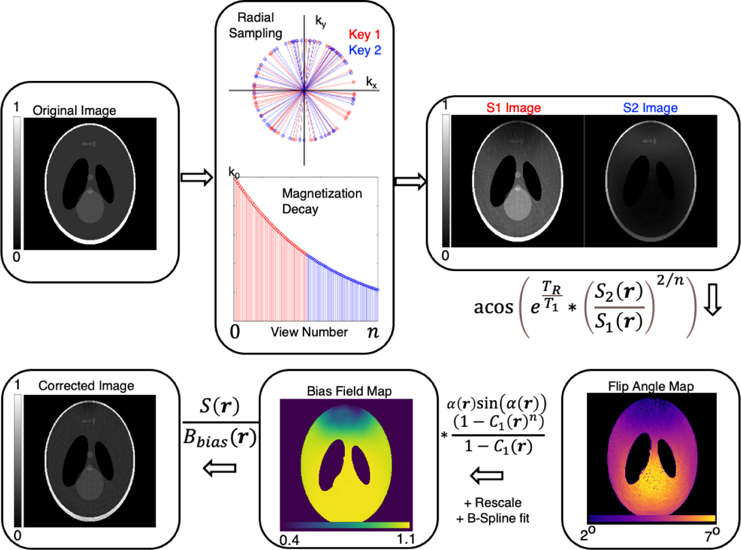
Overview of RF-depolarization mapping using a Shepp-Logan phantom and simulated RF inhomogeneity. The randomly acquired radial views are divided into first and second-half temporal subdivisions and reconstructed separately. The ratio of the two is taken to calculate a flip angle map, which in turn is used to calculate a bias field map. This map is then divided into the fully sampled, but uncorrected image to generate a final bias-corrected image

2.2 |. Template-based correction

Depolarization maps from a cohort of subjects can be subsequently combined to generate a single template flip angle map. This, in combination with knowledge of the point in the trajectory at which a sequence samples the center of k-space, can be used to generate a bias field map for an arbitrary acquisition. The approach is described in Figure 2, which begins with a first depolarization-derived flip angle map to seed the template α_template(r). It is associated with a corresponding thoracic cavity mask m_template(r), to which subsequent flip angle maps and their associated thoracic cavity masks are then rigidly registered. Because the flip angle map is typically slowly spatially varying and fixed for a given coil configuration, registered flip angle maps can then be averaged together to create a final α_template(r).

FIGURE 2.

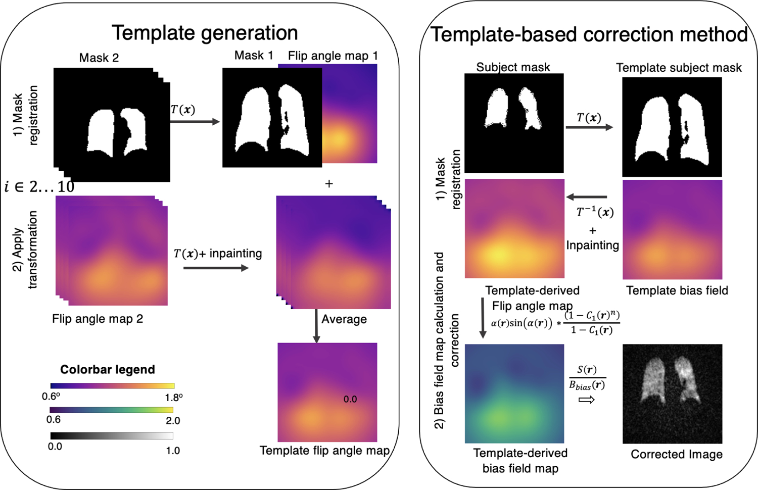
(Left) Process of generating a flip angle mask illustrated with 2 subjects for simplicity. The target mask 1, is arbitrarily chosen as the reference frame to which all others are volumetrically registered. The same registration required to align the subject masks is applied to align the measured flip angle maps. Each registered flip angle map is then inpainted to smooth out any edge effects and averaged into the broader template map. (Right) Illustration of template-based bias field correction. First, the template mask is registered to the subject mask, and the same transformation is then applied to the flip angle template. Inpainting is used to fill in dark boundary areas at the boundary caused by the transformed volume moving partially out of the FOV. The bias field map is calculated using Equation (9). Upon normalization to create the relative template-derived bias field map, the corrected image can be calculated using Equation (10)

Such a template can then be used to correct the images of any desired subject by first registering its template mask to that of the subject,

$$m_{\text{template }}(r)=m_{\text{subject }}(T(r)),$$ (7)

where T(r) is the mapping function determined by the registration process. The inverse of T(r) is then applied to the flip angle map template to transform it into subject’s image space,

$${\alpha }_{\text{subject }}(r)={\alpha }_{\text{template }}\left(T^{-1}(r)\right).$$ (8)

The resulting flip angle map once adjusted to the specific subject, α_subject(r), is then transformed into a bias field map for radial or Cartesian acquisitions using

$$B_{\text{bias,subject }}(r)\propto \{\begin{array}{cc}{\alpha }_{\text{subject }}(r)\text{sin}\left({\alpha }_{\text{subject }}(r)\right)\frac{1-C_1{(r)}^n}{1-C_1(r)}& \text{ Radial }\\ {\alpha }_{\text{subject }}(r)\text{sin}\left({\alpha }_{\text{subject }}(r)\right)C_1^{n_0}& \text{ Cartesian }\end{array}.$$ (9)

It is important to note that for multi-slice, Cartesian imaging, the image SNR is proportional to the signal at the n₀-th excitation, representing the central line of k-space. With this estimate of the bias field, its inverse is applied to the subject’s uncorrected signal distribution S(r),

$$S_{\text{corrected }}(r)=S(r)/B_{\text{bias,subject }}(r),$$ (10)

to yield S_corrected(r), is the bias-field corrected image; the process is graphically depicted in Figure 2.

3 |. METHODS

3.1 |. Simulations

To illustrate the principles of using RF-depolarization for bias-field mapping, simulations were performed using a uniform cylindrical phantom in a field of view that was parsed into a 128 × 128 × 128 matrix. The digital structure was Fourier-transformed to generate k-space data, which was radially sampled and subjected to inhomogeneous RF-induced magnetization decay by imposing a flip angle map regionally varying between 0.5° and 0.8°. The simulation was conducted first in the absence of longitudinal relaxation (T₁ = ∞) and then for representative O₂ concentrations (detailed in the next section) that might be encountered in vivo (T₁ = 10 s in the extreme limit of a patient receiving supplemental oxygen, T₁ = 40 s and in the limit of one with small lung volume, inhaling a large volume of anoxic gas). The digital phantom was radially sampled with 10 000 radial spokes (128 points/spoke), using a 3D randomized Halton spiral pattern²⁷ for a total of a simulated 10 s scan duration (T_R = 0.1 ms). Note, that the digital T_R was adjusted to 0.1 ms to preserve the same relationship between O₂-induced T₁ and scan duration as for in vivo imaging. Images were reconstructed using a conjugate-gradient non-uniform fast Fourier transform (NUFFT) technique²⁸ with an optimized iterative density compensation method.²⁹ The RF-depolarization map was generated as described above and converted to a bias field estimate that was used to recover the corrected image.

3.2 |. In vivo imaging

3D radial ventilation MRI was available for use from 51 subjects (18 healthy, 11 interstitial lung disease, 2 lung transplant, 2 chronic obstructive pulmonary disease [COPD], 11 being evaluated for pulmonary hypertension, 7 radiation therapy) who had undergone imaging in the supine position at 3T (Siemens Magnetom Trio Scanner VB19 - Siemens Healthineers, Erlangen, Germany) using the following parameters: TR/TE = 4.5/0.45 ms; flip angle = 1.5; FOV = 40 cm views = 3600; samples/view = 128. Images were acquired using a quadrature flexible ¹²⁹Xe chest coil (Clinical MR Solutions, Shadybrook, WI). This widely used coil is optimal for patient comfort, but exhibits signal deficits resulting from the cut-outs that accommodate the patient’s arms. Each image acquisition had an image SNR >8 determined using the equation below for magnitude reconstruction,

$$\text{SNR}=\frac{{\text{Mean}}_{\text{signal }}}{\text{ Median }\left({\text{Std}}_{\text{noise per cube }}\right)}\times 0.66,$$ (11)

where Std_{noise per cube} is the average standard deviation of 8 × 8 × 8 cubes inside the thoracic cavity.³⁰

The protocol was approved by the Institutional Review Board of Duke University Medical Center (Durham, NC). The 3D volumes were acquired using a randomized 3D Halton spiral radial sequence and the 2 keys were reconstructed to a Cartesian 128 × 128 × 128 matrix using a kernel sharpness of 0.16. This resulted in images with low-resolution, but high-SNR to achieve a smoothly varying flip angle map. Subsequently, the entire dataset was reconstructed again using a sharpness of 0.32 to provide a higher resolution image for visualizing regional ventilation.

To test the template correction approach on a more standard Cartesian acquisition,²⁷ it was also used to correct a representative 2D gradient-echo (GRE) ventilation image acquired with bandwidth = 170 Hz/pixel, FOV = 38.4 × 36 cm, flip angle = 10°, TR/TE = 7.65/3 ms, and resolution = 4 × 4 × 12 (mm³).

3.3 |. T₁ estimation

RF-depolarization mapping used an estimated ¹²⁹Xe T₁ in the lung that was assumed, based on prior studies, to be dominated by paramagnetic oxygen.³¹ For ¹²⁹Xe-O₂ collisions at 37°C body temperature, ¹²⁹Xe relaxation is approximately linear with O₂ partial pressure $P_{O_2}$³²

$$\frac{1}{T_1}=0.421{\text{s}}^{-1}\cdot {\text{atm}}^{-1}{P}_{O_2}.$$ (12)

$P_{O_2}$ was assumed to be 104 mm Hg³³ or 0.137 atm at end-expiration (functional residual capacity [FRC]) before subjects inhaled an anoxic dose volume of V_dose, therefore, further diluting the oxygen partial pressure to,

$$P_{O_2}=0.137\text{atm}\cdot \frac{\text{FRC}}{\text{FRC}+V_{\text{dose }}}.$$ (13)

This dilution value was calculated for each subject individually, either from measured FRC, if available, or an estimated value if not. For healthy subjects, FRC was estimated using the equation recommended by the European Respiratory Society,³⁴ which for patients with lung disease was scaled down by the ratio of measured versus predicted forced vital capacity.³⁵ For a typical subject with FRC = 3 L, inhaling a 1-L dose, the partial pressure of oxygen after dose inhalation would be ¾ of that at FRC or ~0.1 atm, yielding a T₁ of ~24 s. Note, that although T₁ can vary somewhat across the lung,^31,36 we have assumed it to be constant here; the impact of this assumption is discussed later.

Once an RF-depolarization map had been calculated using a subject-specific T₁ estimate, it was then smoothed with an approximating B-spline²⁶ (spline order = 3; number of levels = 4 × 4 × 4; number of control points = 4 × 4 × 4) and then used to correct the image.

3.4 |. Template-based correction

The flip angle map template was generated using RF-depolarization maps from a subset of n = 10 randomly selected subjects (Figure 2) who had undergone 3D radial ¹²⁹Xe ventilation MRI. Beyond this sample size, addition of each new map to the template changed the sum-of-squares difference from the prior iteration by <1%. For each subject, the thoracic cavity mask was registered using Advanced Normalization Tools³⁷ to a common coordinate system (Mutual Information metric, gradient step = 0.1, 4 resolution levels with 100 × 50 × 25 × 10 iterations per level using shrink factors of 8 × 4 × 2 × 1) and the corresponding transformations were applied to the subject’s RF-depolarization derived flip-angle map. After the transformation and in-painting,³⁸ the flip angle maps were averaged to form a template. The flip angle map template was then registered to the thoracic cavity of the subject whose scan was to be corrected.

3.5 |. Image display and statistical analysis

Ventilation images were rescaled by the top (99th) percentile of intensities and displayed in grayscale.³⁹ All maps were displayed using perceptually uniform sequential colormaps in which the flip angle map, with units of degrees, was displayed with the Magma colormap and the associated bias field (rescaled to a mean value of 1) was displayed using the Viridis colormap. For each of the estimation methods, the resulting bias field was quantified by its range and standard deviation. Similarly, for each of the 3 bias field correction methods, the resulting ventilation distributions were characterized by their mean and coefficient of variation. The spatial variation of corrected ventilation was then analyzed by linear regression of the average intensity as a function of position and rescaled by global average intensity to determine both posterior–anterior and superior–inferior gradients. Overall differences in bias field metrics and imaging metrics were tested for statistical differences using a repeated-measures ANOVA, whereas individual differences were compared using a one-way analysis of variance with a Tukey’s honestly significant difference test. All data and image analyses were completed in MATLAB (The MathWorks, Natick, MA).

4 |. RESULTS

4.1 |. Phantom simulations

Figure 3 depicts the key steps and outcomes of bias field correction using RF-depolarization mapping in a homogeneous digital phantom. The uncorrected reconstruction demonstrates the signal intensity variation that was caused by the application of the deliberately inhomogeneous flip angle map. Here, the upper left quadrant of the image exhibits lower signal intensity, driven by the lower simulated flip angle in that region. Conversely, the lower right quadrant exhibits higher image intensity, driven by the larger simulated flip angle in that region. These effects can be separated by using 2 key images S₁ and S₂ to produce a depolarization map where regions with greater/lower coil sensitivity experience more/less decay as manifested in the S₁/S₂ ratio. The depolarization map is transformed into a flip angle map through Equation (4), and subsequently a bias field map through Equation (5). The bias field map is then used to correct the image using Equation (6) and recovers a homogeneous image as evidenced by the resulting line profile.

FIGURE 3.

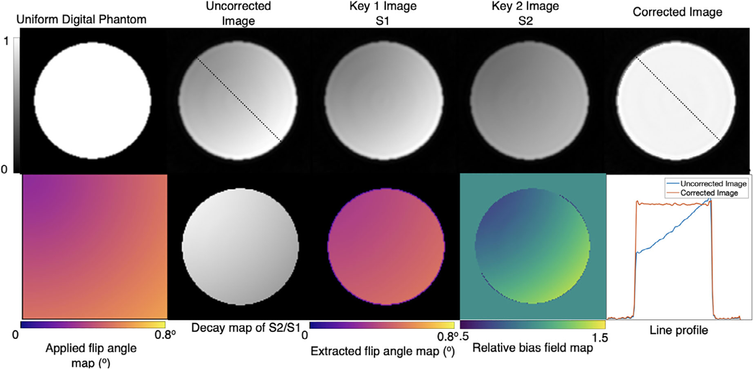
Digital simulation of RF-depolarization mapping of a uniform cylindrical phantom. A simulated B₁ inhomogeneity is applied using the flip angle map, resulting in non-uniform signal intensity variation in the uncorrected reconstruction. Using the 2 keys, a flip angle map is recovered and transformed into a relative bias field map, which when divided into the uncorrected image accurately recovers the underlying uniform signal distribution. The line profiles from the traces in columns 2 and 5 show the effects of the non-uniform flip angle and its successful correction

Figure 4 illustrates the importance of including relaxation effects beyond those caused by RF pulsing by simulating the effects of different global T₁ values on the ability to recover the homogenous line profile. As T₁ becomes shorter, the amount of signal intensity variation imposed by the simulated flip angle map increases across the digital phantom, despite the recovered flip angle map matching that of the one applied. These effects are most readily seen in the bias field map, where the intensity variation imposed by B₁ inhomogeneity is further accentuated by the shorter T₁ because of its influence on the C₁ term in Equation (5). Therefore, if one incorrectly assumes that T₁ = ∞, or is practically very long, this causes the recovered image to remain inhomogeneous, as shown in column 4. For the case of T₁ = 10 s, leaving out T₁ correction results in a negligible bias field removal and, therefore, minimal alteration to the original uncorrected image; this remains relatively true even for T₁ = 40 s. However, when the correct simulated T₁ is used to calculate the bias field map, the homogeneous image and flat line profiles are recovered as in columns 5 and 6.

FIGURE 4.

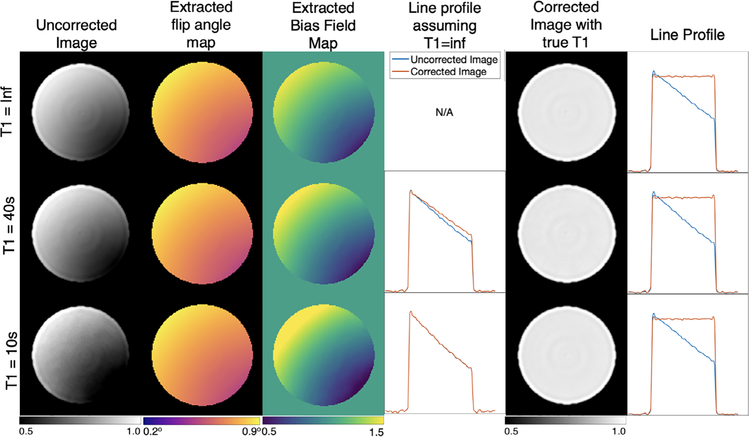
Digital phantom simulation with additional longitudinal relaxation values of T₁ = 10 s and 40 s. Note, that incorrectly assuming infinite T₁ results in an inadequate correction when T₁= 40 s, and a nearly absent one for the T₁=10 s scenario (column 4). However, once an appropriate T₁ value is included, the uniform phantom is recovered in all cases (column 6)

4.2 |. In vivo imaging

In humans, the imaging time becomes comparable to the ¹²⁹Xe T₁, which must therefore be appropriately estimated to correctly separate the RF-induced and T₁-induced depolarization. In our cohort of subjects, using their individual values of FRC (2.98L ± 0.88) and anoxic dose volumes delivered (0.89L ± 0.19), the averaged O₂-induced longitudinal relaxation time was estimated to be to be T₁ = 22.8s ± 2.0. For each subject, estimated T₁ was incorporated to generate a subject-specific bias-field and bias-corrected images. Figure 5 shows an example of a healthy subject’s uncorrected image, which exhibits both high intensities in the right middle lobe and a signal drop-off in the lung apex. This signal deficit is a known effect attributed to the cut-outs for the patient’s arms in the flexible coil architecture. This stands in contrast to birdcage coil designs that offer better B₁-homogeneity, but reduced patient comfort. For this subject, the extracted mean flip angle was 1.18° ± 0.14, corresponding to a ~ 24% variability across the map. When combined with this subject’s estimated T₁ of 21 s, it yielded a bias field map with 32% variation. In this example, the bias field was ~0.8 in the low-intensity apex, versus ~1.3 in the right mid-lung hotspot. On dividing out the bias field, the resulting corrected images showed a pronounced visual change in the rescaled ventilation with the apex signal; it increases from 0.22 to 0.28 in the lung apex, while decreasing from 0.49 to 0.34 in the base.

FIGURE 5.

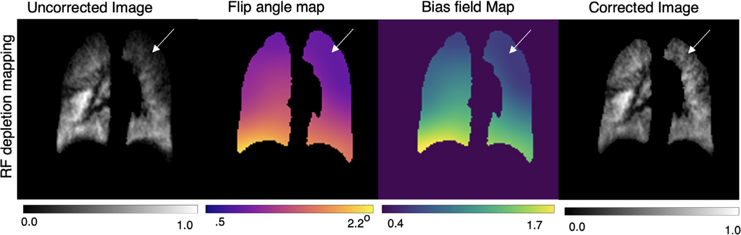
Bias field correction of a healthy subject imaged with 3D radial ¹²⁹Xe MRI using RF-depolarization mapping. Inhomogeneous signal intensity is visually apparent in the apex of the lung (arrows), where low signal is likely because of the arm cutouts in the surface chest coil. Application of the bias field correction recovers the signal in this area

Figure 6 shows a second subject in which we compare the results of bias field correction using the RF-depolarization, template, and N4ITK-based approaches. For RF-depolarization mapping, the recovered flip angle map ranged from 1.10° ± 0.26, and relative bias field ranged from 0.92 ± 0.25. The template-based method recovered a flip angle map ranging from 1.00° ± 0.16, and a relative bias field that ranged from 0.84 ± 0.21. The template-corrected image is visually similar to the one resulting from direct RF-depolarization mapping, with increased intensity at the lung apex after correction. Interestingly, the bias field resulting from depolarization mapping in this subject suggests a higher coil sensitivity near the diaphragm of the right lung. However, such enhanced sensitivity is not seen in the template derived bias field. This difference is possibly caused by motion near the diaphragm during the breath-hold. Such motion breaks the assumption that the gas distribution remains static during imaging and, therefore, has the potential to overestimate the bias field. Finally, the bottom row shows the effect of the N4ITK algorithm that returned a significantly higher relative bias field of 0.95 ± 0.17. Interestingly, the N4ITK method recovers similar spatial features of lower sensitivity at the lung apex, but differs slightly in magnitude at that location, yielding a smaller correction.

FIGURE 6.

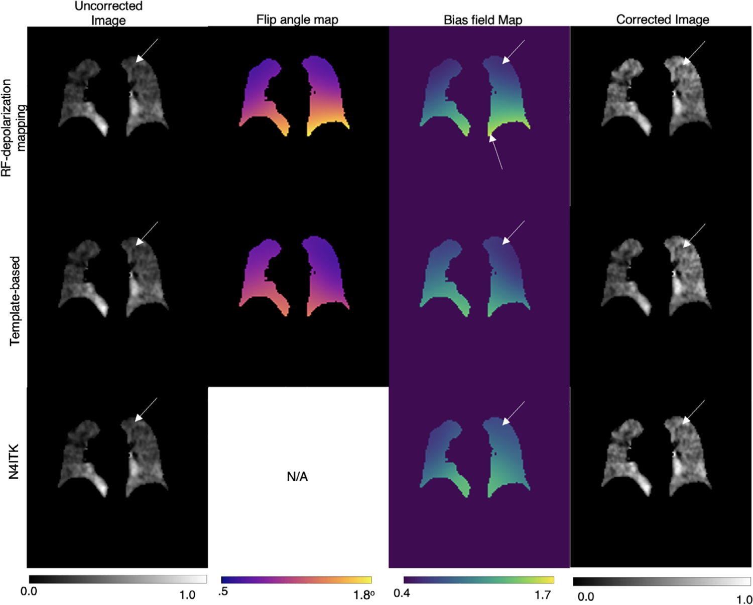
Visual comparisons of bias field correction methods on an NSIP subject with no significant ventilation defects. The flip angle map derived from direct RF-depolarization mapping and that derived from template-based estimation are similar in range, with both methods correcting for the low coil sensitivity in the lung apex. Although N4ITK exhibits a similar spatial pattern, the magnitude of the bias field is visually higher in the lung apex compared to the other 2 methods, resulting in a slightly milder correction there

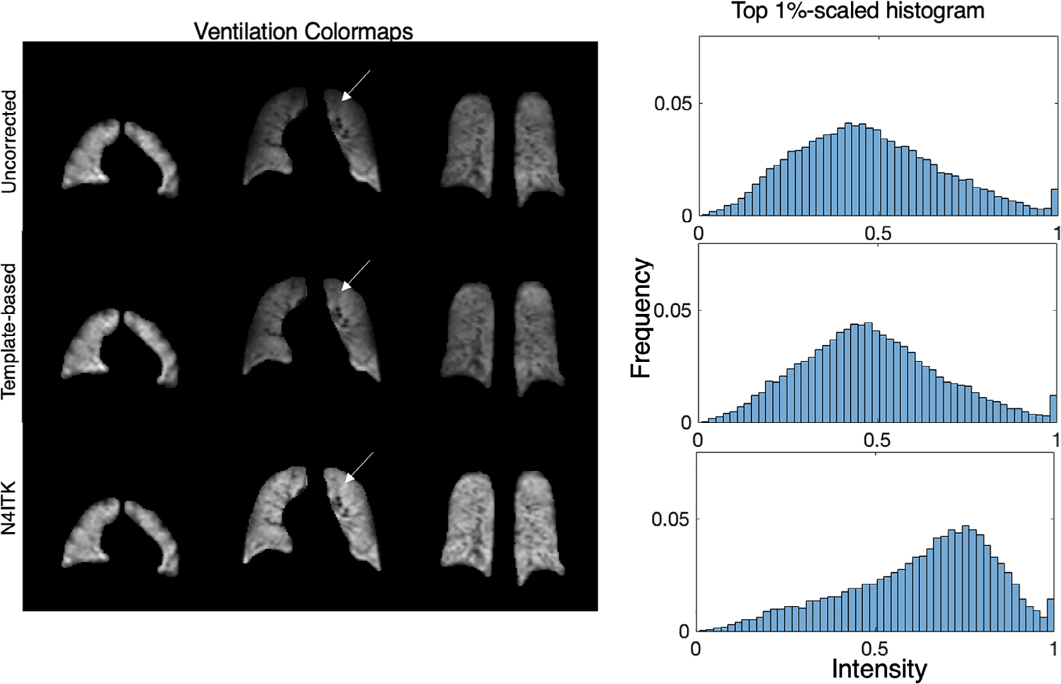
Figure 7 shows multiple slices from a single subject comparing uncorrected, depolarization-based, template-based, and N4ITK methods of bias field correction. The images are displayed using the established ventilation binning color scale to highlight differences between the methods. Note, that all maps are using binning thresholds derived from a healthy cohort originally corrected using the N4ITK method.³⁹ The uncorrected image panel demonstrates signal intensity increasing in both the anterior to posterior and superior to inferior directions. The low signal in the apex of the lung is highlighted by the orange and red color and transitions to green and blue toward the lung base. On application of the RF-depolarization-derived bias field correction, the colormap preserves these features, but the relative intensity in the lung apex and parts of the middle coronal slice has been increased. This is also seen after applying the template-based correction, suggesting that this approach similarly characterizes both the degree of variation and its distribution. However, the N4ITK bias field correction completely removes the perceived signal inhomogeneity, showing only “normal” ventilation with these default thresholds. Shown to the right of these corrected images are the top-percentile rescaled signal distribution histograms. Here, we see that both depolarization- and template-based correction methods affect the histogram modestly, whereas N4ITK shifts the histogram quite dramatically from its uncorrected mean of ~0.3 to a value of ~0.5. Note, although depolarization and template-based corrections largely preserve the histogram shape, they nonetheless reduce inhomogeneity in the colormap.

FIGURE 7.

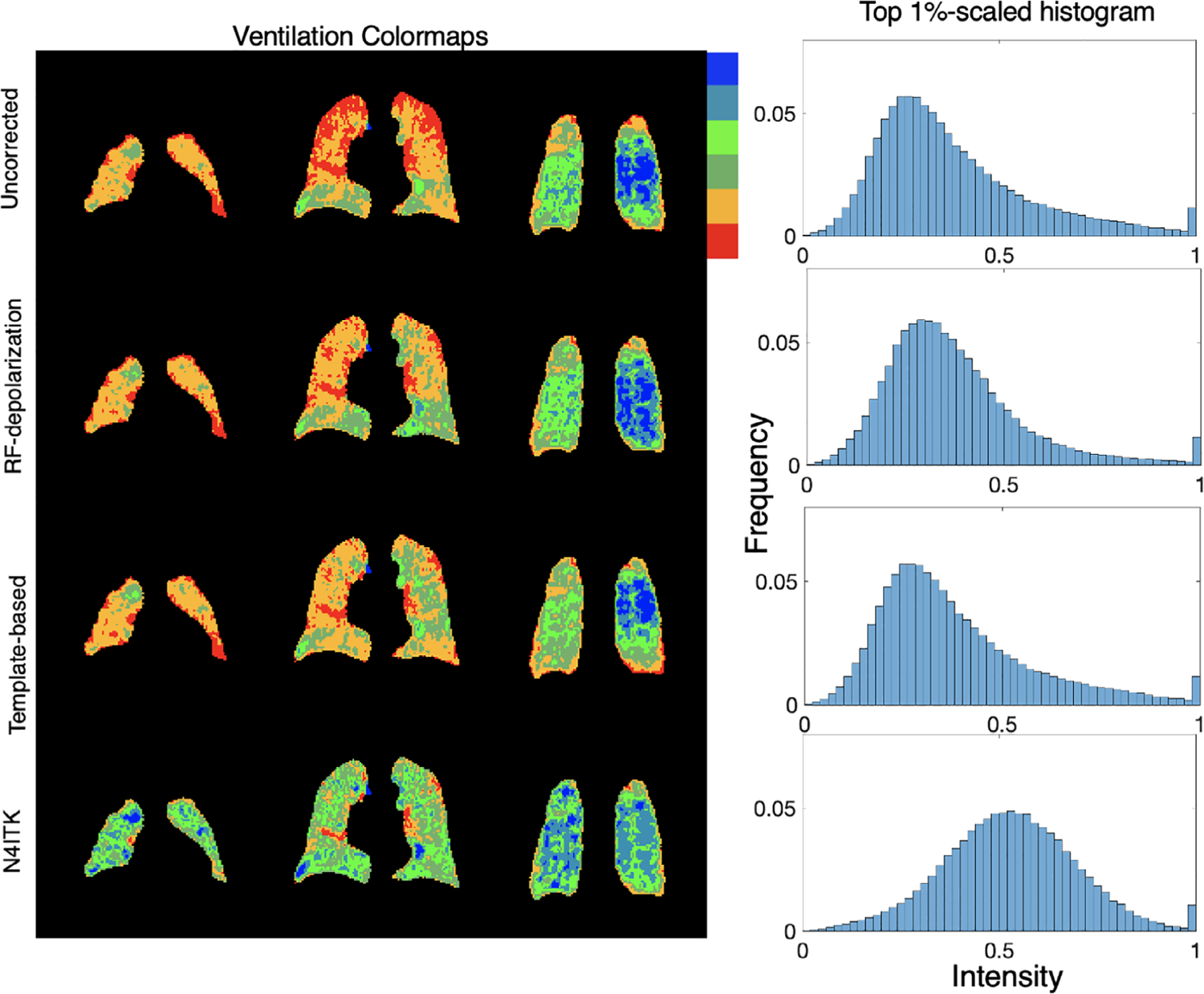
Comparison of 3D radial ventilation maps and histograms resulting from using each of the 3 correction approaches. RF-depolarization mapping and template-based methods achieve similar levels of correction while minimally shifting the histogram mean. By contrast, direct application of N4ITK confers a more aggressive correction that significantly shifts the overall histogram to higher intensities. Note, that all color maps are depicted using binning thresholds derived from the original N4ITK corrected cohort they are intended only to visualize differences, not to indicate what is “normal”

These observations in Figure 7 are seen on a cohort-wise basis in Figure 8 where the ventilation distribution mean after N4ITK correction is significantly higher than the other 3 methods (P < 0.001 for each comparison). The figure also shows that all 3 approaches reduce the amount of intensity variation across the image as measured by the coefficient of variation (RF-depolarization: P = 0.044, template: P = 0.012, N4ITK: P < 0.001). However, N4ITK yields image distributions with the lowest coefficient of variation (P < 0.001), whereas RF-depolarization and template-based correction produce ventilation distributions that do not significantly differ from one another (P = 0.99). None of the 3 methods exhibit significant differences from one another in the 90th-10th percentile range (P = 0.18) and standard deviation (P = 0.31).

FIGURE 8.

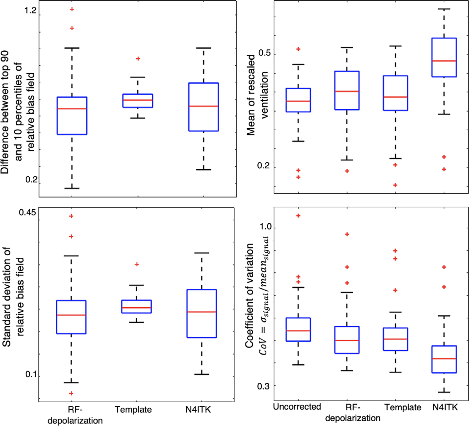
Quantitative comparison of derived bias fields (left) and ventilation distributions (right) across the entire cohort. There was no significant difference between the top 90—top 10 percentile difference or overall standard deviation across any of the bias field maps. However, for the resulting ventilation maps, the N4ITK algorithm significantly shifts the mean of the rescaled distribution to a higher value (P < 0.001). Moreover, all the correction methods significantly decrease the coefficient of variation of the resulting ventilation distribution (RF-depolarization: P = 0.044, template: P = 0.012, N4ITK: P < 0.001)

Figure 9 illustrates the anterior–posterior and superior–inferior gradients in the corrected ¹²⁹Xe signal distributions for healthy subjects. It shows both the line profiles for an individual representative subject as well as the population mean gradient in these directions for each of the correction approaches. The line profiles show the uncorrected intensity distribution to have a strong anterior–posterior gradient, which is somewhat moderated by both the depolarization- and template-based corrections. However, this gradient is eliminated by the N4ITK algorithm. In the superior–inferior direction, the uncorrected image again exhibits a strong gradient, which this time is largely, although not completely, eliminated by all 3 correction approaches. In aggregate, the uncorrected images exhibited a positive anterior–posterior gradient of 2.23 ± 2.95%/cm, which was only very slightly moderated by the RF depolarization, and template-based corrections to 2.77 ± 2.09%/cm and 2.01 ± 2.73%/cm, respectively. In contrast, this gradient was completely removed by the N4ITK algorithm (P <0.002) to −0.04 ± 1.58%/cm. In the superior–inferior direction, only the uncorrected image exhibited a significant positive intensity gradient of 3.35 ± 2.05%/cm, whereas the RF depolarization, template, and N4ITK corrected images had their gradients diminished to 0.17 ± 2.65, −0.78 ± 2.14, and 0.60 ± 0.91%/cm, respectively (P < 0.001 for each comparison).

FIGURE 9.

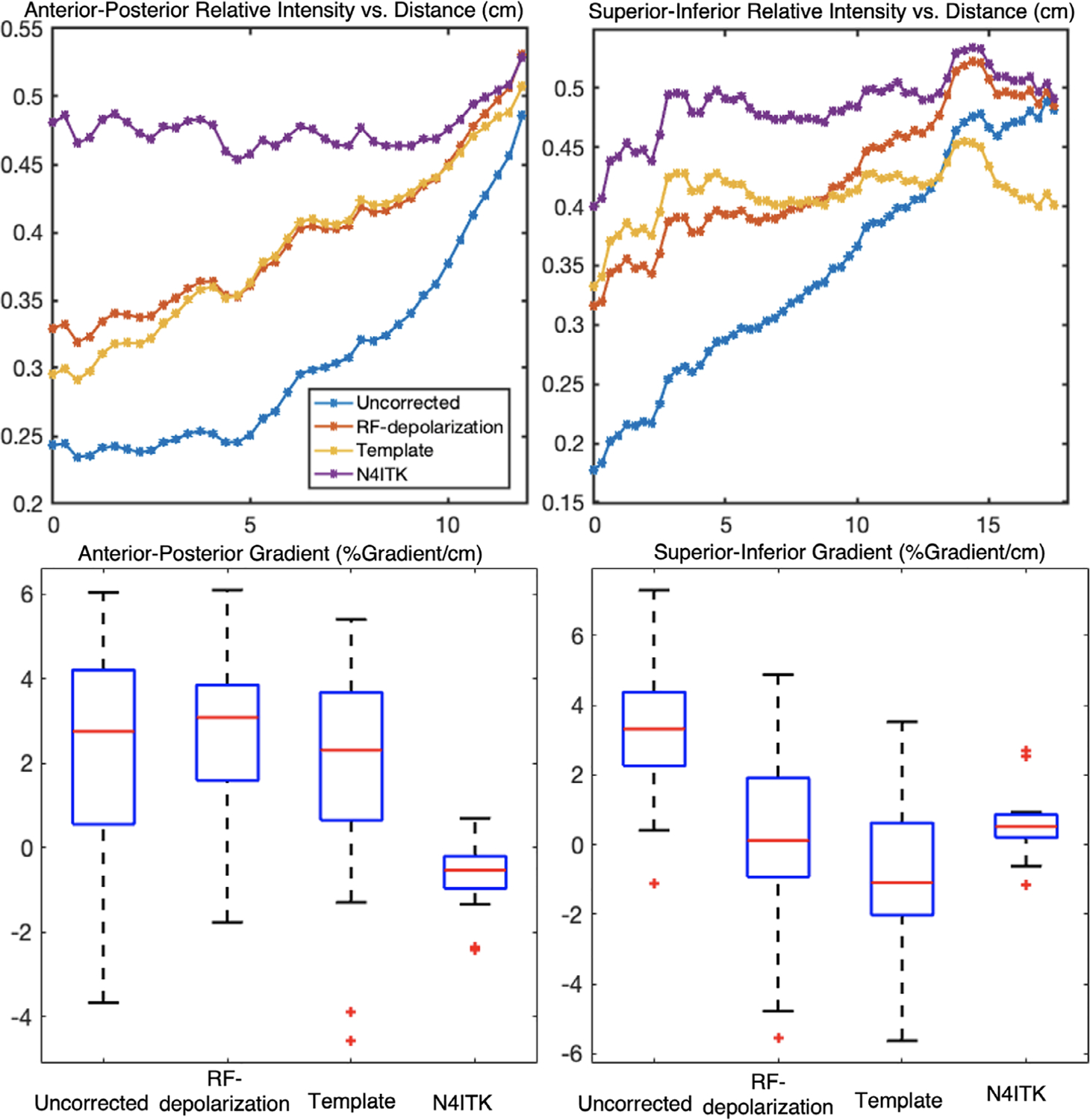
Top: line profile showing ventilation gradients in a representative healthy subject in the anterior–posterior and superior–inferior directions. Bottom: gradients (%gradient/cm) of healthy subjects (n = 18) in the cohort in the anterior–posterior and superior–inferior direction. In the anterior–posterior direction, both the depolarization and template-based correction methods preserved the gravitational gradient, whereas N4ITK eliminated this gradient entirely (P < 0.001). By contrast, gradients in the superior–inferior direction were significantly removed by each of the methods compared to the uncorrected image (P < 0.001)

Figure 10 demonstrates the extension of using the flip angle map template to correct a more commonly used 2D GRE image from a healthy subject. The images are displayed in grayscale to highlight the subtle differences of each method. To enable this correction, the anisotropic mask from the 2D GRE multi-slice image was first resampled and registered to the spatially isotropic 3D flip angle map template. After using this to calculate the subject’s specific flip angle map in the isotropic resolution, it was transformed back to its original 2D resolution and used for slice-by-slice calculation of the bias field. Applying this correction demonstrates that the mean of the rescaled ventilation distribution was only slightly affected using the template-based bias field from 0.47 to 0.48, whereas N4ITK significantly shifted the mean to 0.69.

FIGURE 10.

Comparison of bias field correction using the template-based approach versus N4ITK on 2D GRE images of a healthy subject. A flip angle map was created registering 2D anisotropic masks to the 3D isotropic mask of the template, applying the approach in Figure 2, rescaling the flip angle map to have a mean of the prescribed 10°, and applying Equation (9) for Cartesian-based bias field correction. Bias field correction using the template did not significantly shift the ventilation distribution mean (0.47 to 0.48), whereas N4ITK significantly shifted the distribution to have a mean of 0.69. The signal inhomogeneity in the superior–inferior is reduced, whereas the high signal in the anterior is preserved

5 |. DISCUSSION

Through digital simulations with deliberate application of an inhomogeneous B₁, we first demonstrated that a randomized radial MRI acquisition combined with the depolarization mapping method can robustly recover the underlying homogenous signal. However, these simulations further demonstrated that for typically expected in vivo conditions, ¹²⁹Xe T₁ relaxation cannot be neglected and must be correctly estimated to recover the underlying signal distribution. If T₁ is underestimated, inhomogeneity will be insufficiently removed. However, because it is impossible to distinguish the effects of longitudinal relaxation versus RF pulsing on the measured hyperpolarized magnetization decay, T₁ must be estimated based on expected O₂ partial pressures. For the subjects in our cohort, the mean T₁ ~22 s agreed well with the value of ~20 s estimated by Mugler et al.²³ It is noteworthy that in patients with lung disease, T₁ could be lower in regions of poor gas exchange where O₂ is extracted more slowly from airspaces. The $P_{O_2}$ mapping studies of Miller et al,²⁴ resulted in an estimated $P_{O_2}$ of ~85 mm Hg for healthy subjects and ~80 mm Hg for diseased subjects, which according to Equation (12), translates to T₁ = 21 and T₁ = 23s, respectively. However, higher $P_{O_2}$ could be found in patients receiving supplemental oxygen during MRI, which Miller showed to be ~120 mm Hg $P_{O_2}$. In our cohort of subjects, the standard deviation of T₁ was small (σ = 2 s, range = 20–27 s) that suggests it may be possible to simply use average a population-wide average T₁ = 22.8 s to generate bias fields. Preliminary analysis shows that such an assumption is benign and does not significantly affect VDP, ventilation gradients, and mean ventilation. This simplifying assumption avoids the need to estimate T₁ on for individual subjects, but must be revisited for those where extreme T₁ values (high or low) are considered to be a possibility. Moreover, although concerns regarding accurate estimation of O₂-induced T₁ are valid for RF-depolarization mapping of individual subjects, these effects are mitigated by averaging across multiple subjects in the template-based method.

With an estimated T₁ value in hand and local flip angle calculated by depolarization mapping, a final bias field map representing total signal attenuation can be extracted for individual subjects. Moreover, these individual flip angle maps can be registered to a common space and formed into a template that can be used to calculate the bias field map for arbitrary pulse sequences beyond the randomized 3D radial acquisition.

Our study revealed that both RF depolarization and template-based correction provide a much less aggressive correction than the commonly used N4ITK method. This is evident in the starkly larger shift N4ITK confers to the rescaled intensity histograms, as well as the significantly reduced coefficient of variation seen in the corrected image. Moreover, the bias field estimated from N4ITK had different spatial features compared to RF depolarization and template-based approaches. Among the most striking features were the effects the various correction methods exerted on the anterior–posterior intensity gradients. Specifically, both the RF depolarization and template-based corrections preserved an anterior–posterior intensity gradient of ~2%/cm in healthy subjects, whereas it was eliminated by N4ITK correction. In contrast, all 3 correction methods reduced inhomogeneity in the superior–inferior direction, which is largely dominated by coil design rather than physiology. Taken together, these findings suggest that N4ITK is applying an overly harsh correction. This is not entirely unexpected given that, by definition, it seeks to reduce all smooth and slowly varying intensities. Therefore, it will eliminate true physiological gradients such as the well-known effects of gravity on ventilation in the supine lung that occur on this spatial scale. In aggregate, our results suggest that the proposed methods successfully eliminate the non-physiologic superior–inferior gradients caused by RF inhomogeneity, but do so while preserving the well-known functional gravitational gradients.^13,40

Although this approach to bias field correction is encouraging, it is also necessary to understand the way it is affected by the propagation of uncertainty. Here, we use the methods of Costa et al,⁴¹ in combination with Equation (4) to identify the determinants of flip angle uncertainty σ_α,

$${\sigma }_{\alpha }=\frac{2C_1{\sigma }_s}{n{S}_1}\sqrt{\frac{\frac{1}{C_1^n}+1}{e^{-\frac{2T_R}{T_1}}-C_1^2}}.$$ (15)

Here, C₁ is defined in Equation (3), n is the number of radial views, σ_s is the noise in both key images, and S₁ is the total signal in key 1. It is possible to gain some intuition to this effect by assuming that T₁ ≫ n × T_R, in which case, the error term is largely dominated by the image SNR of S₁/σ_s, as well as the number of radial views, n. Using average values that are representative of this study, the estimated uncertainty in the derived flip angle at a given voxel is ~11%. However, this does not yet consider the smoothing that is applied in generating the bias field map. Considering a simplistic averaging the neighboring voxels, reduces the relative flip angle uncertainty by $\sqrt{27}\approx 5.2$ to ~2%. Propagating this further into Equation (9) for bias field reveals approximately a 22% error, but 4% in the above case of smoothing. For the case of 2D Cartesian images, there will be additional uncertainty caused by the error in registering the mask to the 3D flip angle template that will require more detailed investigations to reliably quantify. However, we note that for 2D imaging, even ~10° flip angles fall within reasonable application of the small-angle approximation, and, therefore, we can expect relatively similar uncertainties to apply in this correction scenario.

Although further work is needed, this approach suggests that a template-based approach may be the optimal way to correct bias field in ¹²⁹Xe ventilation MRI. We expect that for centers using the same coil architecture, the existing template and mask could be used regardless of scanner vendor. If different coil architecture is used, such as the homogeneous birdcage design, it would be necessary to acquire depolarization maps in 5–10 volunteers to build an appropriate flip angle template. With increasing confidence in the veracity of bias field corrections, the community would have the opportunity to more vigorously pursue biomarkers associated with aspects of the ventilation distribution beyond the well-known ventilation defect percentage. For example, recent work by Hahn et al⁴² has shown that high ventilation percentage is an intriguing biomarker of progression in fibrotic lung disease.

5.1 |. Study limitations and opportunities for refinement

Calculating the bias field via RF-depolarization mapping has several limitations. First, the method currently requires estimating the ¹²⁹Xe T₁ and assuming it to be uniform over the entire lung. We know this to be overly simplistic because studies have shown that T₁ can be heterogeneous, especially in subjects with disease.³⁶ One approach to improving the accuracy of the bias field measurement is to build templates using only healthy volunteers, in whom T₁ heterogeneity should be minimal. The approach could further be improved by incorporating a second scan to directly measure global T₁ rather than estimating it. Of note, dissemination of this approach for quantitative ventilation analysis would require re-analyzing previously published ventilation reference distributions to establish new binning thresholds.³⁹

Furthermore, the method assumes that the true flip angle map stays constant for a given coil configuration, therefore, ignoring effects such as coil shape, patient positions relative to the coil, and RF loading. This effect was investigated by using patient weight as a proxy for such effects and discovered that this had no correlation to either mean extracted flip angle (r² = 0.02) or flip angle map variation (r² = 0.02). This suggests that such patient-specific effects are likely to be minimal except perhaps in the most extreme cases of suboptimal coil shape.

Moreover, to translate the template to multiple acquisitions often acquired at different prescribed flip angles, we must assume that the coil behaves linearly. An additional assumption in using a flexible quadrature chest coil is that the 2 coil pairs are exactly in quadrature. If the RF fields per unit current of each coil pair are not orthogonal to one another, they can produce artifacts that are manifested by signal non-uniformity,⁴³ which is not accounted for in the model of RF-depolarization mapping.

Given that the proposed bias field correction methods preserve physiologic features such as gravitationally induced, heterogeneity, it is reasonable to speculate whether quantification calculation of metrics such as VDP, derived using linear binning techniques will require adjustment. Specifically, for 3D images, the ventilation distribution in posterior slices may be skewed toward a higher mean value than those in the anterior lung. We anticipate that once reference distributions have been updated with the proposed methods for bias field correction, this can be more thoroughly tested against expert reader assessments.⁴⁴

6 |. CONCLUSION

Here, we have demonstrated a means for mapping ¹²⁹Xe flip angle and bias field that can correct for RF inhomogeneity while leaving physiological gradients intact. This approach requires randomized 3D radial acquisitions, but has been extended to produce a flip angle map template that can be applied to arbitrary sequences. Both techniques demonstrate similar image corrections that better preserve physiologic gradients than what is obtained with retrospective correction techniques like N4ITK. Although accurately estimating the bias field for functional ¹²⁹Xe ventilation images remains challenging, the approach described here should provide a useful means to improve the precision with which this problem can be addressed. With improved and more repeatable bias field correction methods, it should be possible to provide an increasingly detailed assessment of the broader ventilation distribution beyond ventilation defects alone.

REFERENCES

- 1.Wang JM, Robertson SH, Wang Z, et al. Using hyperpolarized 129Xe MRI to quantify regional gas transfer in idiopathic pulmonary fibrosis. Thorax. 2018;73:21–28. [DOI] [PMC free article] [PubMed] [Google Scholar]
- 2.Virgincar RS, Cleveland ZI, Sivaram Kaushik S, et al. Quantitative analysis of hyperpolarized 129Xe ventilation imaging in healthy volunteers and subjects with chronic obstructive pulmonary disease. NMR Biomed. 2013;26:424–435. [DOI] [PMC free article] [PubMed] [Google Scholar]
- 3.Thomen RP, Walkup LL, Roach DJ, Cleveland ZI, Clancy JP, Woods JC. Hyperpolarized 129Xe for investigation of mild cystic fibrosis lung disease in pediatric patients. J Cyst Fibros. 2017;16:275–282. [DOI] [PMC free article] [PubMed] [Google Scholar]
- 4.Wang Z, Bier EA, Swaminathan A, et al. Diverse cardiopulmonary diseases are associated with distinct xenon magnetic resonance imaging signatures. Eur Respir J. 2019;54:1900831. [DOI] [PMC free article] [PubMed] [Google Scholar]
- 5.Svenningsen S, Kirby M, Starr D, et al. Hyperpolarized 3 He and 129Xe MRI: differences in asthma before bronchodilation. J Magn Reson Imaging. 2013;38:1521–1530. [DOI] [PubMed] [Google Scholar]
- 6.He M, Wang Z, Rankine L, et al. Generalized linear binning to compare hyperpolarized 129Xe ventilation maps derived from 3D radial gas exchange versus dedicated multislice gradient echo MRI. Acad Radiol. 2020;27:e193–e203. [DOI] [PMC free article] [PubMed] [Google Scholar]
- 7.Tustison NJ, Altes TA, Qing K, et al. Image- versus histogram-based considerations in semantic segmentation of pulmonary hyperpolarized gas images. Magn Reson Med. 2021;86:2822–2836. [DOI] [PubMed] [Google Scholar]
- 8.Song S, Zheng Y, He Y. A review of methods for bias correction in medical images. Biomed Eng Rev. 2017;3:1–10. [Google Scholar]
- 9.Mihara H, Iriguchi N, Ueno S. A method of RF inhomogeneity correction in MR imagingblower rtx 3090. Magn Reson Mater Phys Biol Med. 1998;7:115–120. [DOI] [PubMed] [Google Scholar]
- 10.Miller GW, Altes TA, Brookeman JR, De Lange EE, Mugler JP. Hyperpolarized 3He lung ventilation imaging with B1-inhomogeneity correction in a single breath-hold scan. Magn Reson Mater Phys Biol Med. 2004;16:218–226. [DOI] [PubMed] [Google Scholar]
- 11.Tustison NJ, Cook PA, Gee JC. N4ITK: improved N3 bias correction. IEEE Trans Med Imaging. 2011;29:1310–1320. [DOI] [PMC free article] [PubMed] [Google Scholar]
- 12.Sied JG, Zijdenbos AP, Evans AC. A nonparametric method for automatic correction of intensity nonuniformity in MRI data. IEEE Trans Med Imaging. 1998;17:87–97. [DOI] [PubMed] [Google Scholar]
- 13.Hopkins SR, Henderson AC, Levin DL, Yamada K, Buxton RB, Prisk GK. Vertical gradients in regional lung density and. Lung. 2008;103:240–248. [DOI] [PMC free article] [PubMed] [Google Scholar]
- 14.Galvin I, Drummond GB, Nirmalan M. Distribution of blood flow and ventilation in the lung: gravity is not the only factor. Br J Anaesth. 2007;98:420–428. [DOI] [PubMed] [Google Scholar]
- 15.Kern AL, Vogel-Claussen J. Hyperpolarized gas mri in pulmonology. Br J Radiol. 2018;91:20170647. [DOI] [PMC free article] [PubMed] [Google Scholar]
- 16.Roach DJ, Willmering MM, Plummer JW, et al. Hyperpolarized 129Xenon MRI ventilation defect quantification via thresholding and linear binning in multiple pulmonary diseases. Acad Radiol. 2022;29:S145–S155. [DOI] [PMC free article] [PubMed] [Google Scholar]
- 17.Niedbalski PJ, Willmering MM, Robertson SH, et al. Mapping and correcting hyperpolarized magnetization decay with radial keyhole imaging. Magn Reson Med. 2019;82:367–376. [DOI] [PMC free article] [PubMed] [Google Scholar]
- 18.Studholme C, Cardenas V, Song E, Ezekiel F, Maudsley A, Weiner M. Accurate template-based correction of brain MRI intensity distortion with application to dementia and aging. IEEE Trans Med Imaging. 2004;23:99–110. [DOI] [PMC free article] [PubMed] [Google Scholar]
- 19.Chen M, Doganay O, Matin T, et al. Delayed ventilation assessment using fast dynamic hyperpolarised Xenon-129 magnetic resonance imaging. Eur Radiol. 2020;30:1145–1155. [DOI] [PMC free article] [PubMed] [Google Scholar]
- 20.Willmering MM, Roach DJ, Kramer EL, Walkup LL, Cleveland ZI, Woods JC. Sensitive structural and functional measurements and 1-year pulmonary outcomes in pediatric cystic fibrosis. J Cyst Fibros. 2021;20:533–539. [DOI] [PMC free article] [PubMed] [Google Scholar]
- 21.Hoult DI, Richards RE. The signal-to-noise ratio of the nuclear magnetic resonance experiment. Ratio. 1976;85:71–85. [DOI] [PubMed] [Google Scholar]
- 22.Stumpf C, Malzacher M, Schmidt LP. Radio frequency modeling of receive coil arrays for magnetic resonance imaging. J. Imaging 2018;4:1–17. [Google Scholar]
- 23.Mugler JP, Altes TA. Hyperpolarized 129Xe MRI of the human lung. J Magn Reson Imaging. 2013;37:313–331. [DOI] [PMC free article] [PubMed] [Google Scholar]
- 24.Miller GW, Mugler JP, Altes TA, et al. Three-dimensional PO2 mapping of human lungs in a short breath hold using hyperpolarized xenon-129. Proc Int Soc Magn Reson Med. 2013;21:1448. [Google Scholar]
- 25.Stadler A, Jakob PM, Griswold M, Stiebellehner L, Barth M, Bankier AA. T1 mapping of the entire lung parenchyma: influence of respiratory phase and correlation to lung function test results in patients with diffuse lung disease. Magn Reson Med. 2008;59:96–101. [DOI] [PubMed] [Google Scholar]
- 26.Tustison NJ, Gee JC. N-D Ck B-Spline Scattered Data Approximation. The Insight Journal; 2006. 10.54294/0d55to [DOI] [Google Scholar]
- 27.Niedbalski PJ, Hall CS, Castro M, et al. Protocols for multi-site trials using hyperpolarized 129Xe MRI for imaging of ventilation, alveolar-airspace size, and gas exchange: a position paper from the 129Xe MRI clinical trials consortium. Magn Reson Med. 2021;86:2966–2986. [DOI] [PubMed] [Google Scholar]
- 28.Lin JM. Python non-uniform fast fourier transform (PyNUFFT): an accelerated non-cartesian MRI package on a heterogeneous platform (CPU/GPU). J Imaging. 2018;4:1–22. [Google Scholar]
- 29.Robertson SH, Virgincar RS, He M, Freeman MS, Kaushik SS, Driehuys B. Optimizing 3D noncartesian gridding reconstruction for hyperpolarized 129 Xe MRI-focus on preclinical applications. Concepts Magn Reson Part A. 2015; 44:190–202. [Google Scholar]
- 30.He M, Zha W, Leith R, Fain S, Driehuys B. A comparison of two hyperpolarized 129Xe MRI ventilation quantification pipelines: the effect of signal to noise ratio. Acad Radiol. 2019;26:949–959. [DOI] [PMC free article] [PubMed] [Google Scholar]
- 31.Deninger AJ, Eberle B, Ebert M, et al. Quantification of regional intrapulmonary oxygen partial pressure evolution during apnea by 3He MRI. J Magn Reson. 1999;141:207–216. [DOI] [PubMed] [Google Scholar]
- 32.Saam B. T1 relaxation of 129Xe and how to keep it long. New Dev NMR. 2015;2015:122–141. [Google Scholar]
- 33.Ortiz-Prado E, Dunn JF, Vasconez J, Castillo D, Viscor G. Partial pressure of oxygen in the human body: a general review. Am J Blood Res. 2019;9:1–14. [PMC free article] [PubMed] [Google Scholar]
- 34.Gommers D. Functional residual capacity and absolute lung volume. Curr Opin Crit Care. 2014;20:347–351. [DOI] [PubMed] [Google Scholar]
- 35.Cooper BG, Stocks J, Hall GL, et al. The global lung function initiative (GLI) network: bringing the world’s respiratory reference values together. Breathe. 2017;13:e56–e64. [DOI] [PMC free article] [PubMed] [Google Scholar]
- 36.Neemuchwala F, Ghadimi Mahani M, Pang Y, et al. Lung T1 mapping magnetic resonance imaging in the assessment of pulmonary disease in children with cystic fibrosis: a pilot study. Pediatr Radiol. 2020;50:923–934. [DOI] [PubMed] [Google Scholar]
- 37.Avants BB, Tustison NJ, Johnson H. Advanced Normalization Tools (ANTS); 2014.
- 38.Bertalmío M, Bertozzi AL, Sapiro G. Navier-stokes, fluid dynamics, and image and video inpainting. Proc IEEE Comput Soc Conf Comput Vis Pattern Recognit. 2001;1:355–362. [Google Scholar]
- 39.He M, Driehuys B, Que L, Yuh-Chin H. Using hyperpolarized 129Xe MRI to quantify the pulmonary ventilation distribution. Acad Radiol. 2016;23:1521–1531. [DOI] [PMC free article] [PubMed] [Google Scholar]
- 40.He M, Robertson SH, Kaushik SS, et al. Dose and pulse sequence considerations for hyperpolarized 129Xe ventilation MRI. Magn Reson Imaging. 2015;33:877–885. [DOI] [PMC free article] [PubMed] [Google Scholar]
- 41.Costa M, Niedbalski PJ, Willmering MM, Cleveland ZI. Optimized magnetization decay correction of hyperpolarized 129Xe ventilation images using. In: ISMRM; 2021:3795. [Google Scholar]
- 42.Hahn AD, Carey KJ, Sandbo ND, et al. Response of hyperpolarized 129Xe MRI measures of ventilation and gas-exchange to antifibrotic treatment in Idiopathic Pulmonary Fibrosis. In: ISMRM & SMRT; 15–50; 2021: 0591. [Google Scholar]
- 43.Redpath TW. Quadrature rf coil pairs. Magn Reson Med. 1986;3:118–119. [DOI] [PubMed] [Google Scholar]
- 44.Ebner L, He M, Virgincar RS, et al. Hyperpolarized 129Xenon magnetic resonance imaging to quantify regional ventilation differences in mild to moderate asthma. Invest Radiol. 2017;52:120–127. [DOI] [PMC free article] [PubMed] [Google Scholar]