Exact Analytical Form of Diatomic Molecular Orbitals

Abstract

We provide the exact analytical form of diatomic molecular orbitals, as given by the solutions of a single-electron diatomic molecule with arbitrary nuclear charges, using our recently developed method for solving Schrödinger equations. We claim that the best representation of the wave function is a factorized form including a power prefactor, an exponentially decaying term, a modulator function on the exponential, and additional factors accounting for nodal surfaces and the magnetic quantum number. Applying our method, we have identified unexpected extreme points along the potential energy curves, hence revealing the limitations of the well-known concepts of bonding and antibonding.

I. Introduction

Since the concept of orbital was proposed in the early days of quantum chemistry, this concept has been widely accepted by chemists as the most powerful theoretical tool to gain deep insight into chemical problems. Although orbitals are based on the independent single-electron picture, which is only an approximation to the correlated many-electron picture described by many-electron wave functions in atoms and molecules, their concise, intuitive, and visualizable features make them the most commonly used terminology in chemists’ routine discussions.

Among various orbitals introduced for different purposes, the most successful ones are undoubtedly the atomic orbitals (AOs) of hydrogenic systems. Rigorously defined as the solutions of a single-electron Schrödinger equation (SE) with spherical symmetry, each of these AOs can be analytically written as a product of a radial function and a spherical harmonic. For many-electron atoms with electron–electron interactions, although one cannot separate variables to deduce single-electron SEs, the clever idea of introducing electronic screening and effective nuclear charge has allowed a reduction to the hydrogenic picture where electrons fill into different energy levels.^1,2 The resulting AOs for many-electron atoms capture the essential physics and have achieved enormous success in explaining the electronic structure of elements in the periodic table.

Yet, chemistry deals with molecules. Apart from understanding AOs, perhaps even more important for chemists is to decipher the molecular orbitals (MOs). In contrast to atoms, molecules display much greater complexity in the presence of multiple electrons and nuclei. The idea of treating electron–electron interactions as an effective screening as used in atoms is not feasible for molecules due to the ambiguity of assigning effective nuclear charges. It turns out that a plausible way is to invoke a fictitious noninteracting system with an effective potential. The resulting MOs can be generated by solving the SE of that particular potential, either local or nonlocal, for example, as has been practiced by the Kohn–Sham density functional theory (KS-DFT)³ or the Hartree–Fock (HF) theory, giving rise to different MOs associated with different methods or different functional approximations in DFT. This ambiguity of MOs can be once again attributed to the attempt at using approximate orbitals to describe a correlated many-electron wave function.

Nevertheless, for single-electron molecules, MOs can be unambiguously defined. For diatomic molecules, in particular, these MOs are named σ, π, δ, etc., in analogy with the s, p, and d types for AOs, and have given tremendous inspiration to chemists. In fact, they have become the most essential part of modern chemistry textbooks.^1,2,4 In contrast to the s, p, and d orbitals whose analytical forms have been clarified, however, the exact analytical forms of MOs remain a challenge. For example, the MOs for the simplest molecular ion, H₂⁺, have been studied intensively, but their compact analytical forms are still elusive.⁵⁻¹⁹ Instead, these MOs are usually numerically represented as linear combinations of atomic orbitals (LCAOs).^20,21

In this paper, we show that we can do better than basis expansion by finding the exact analytical forms of all the MOs. In particular, we apply our recently developed method for solving SEs to single-electron diatomic molecules and derive the exact expressions for σ, π, δ orbitals and so on. For each MO, our formula is in an exactly factorized form, i.e., casting the wave function into a product of multiple factors resembling the exact formula of an AO. This is in contrast to the conventional LCAOs and other basis expansion methods that decompose the wave function into a sum of infinite terms. Our representation of MOs reveals their intrinsic analytical structure and furthermore has proven to have computational advantages, as shown in our recent work.²² Importantly, the newly obtained analytical form of MOs could give us new insight into the nature of chemical bonds.

II. Methods

We start by reviewing our newly proposed method for solving one-dimensional (1D) SEs, as has been implemented for finding the exact analytical solutions of 1D hydrogen atom and H₂⁺ with soft Coulomb potentials.^23,24 In particular, for a nicely behaved potential in 1D, by formulating the corresponding ground state wave function as ψ = Ce^β, we can transform the SE for ψ(x) into a Riccati equation²⁵ for , where energy enters as a parameter. In doing this, we reduce the second-order ordinary differential equation (ODE) into first-order at the sacrifice of linearity. The equation is then solved by expanding u into a Taylor series, which combined with the boundary conditions ultimately leads to an algebraic equation that determines the energy.^23,24 In this work, we extend our approach to real-world molecules in 3D. As will be shown, the increased dimensionality leads to an increase in the number of algebraic equations and unknown variables, yet the basic structure remains similar.

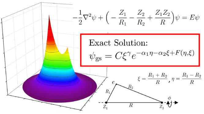
Without loss of generality, let us consider the generic single-electron diatomic molecular problem in atomic units:

1

Here R_i’s are the electron–nuclear distances, R is the nuclear separation, and Z_i’s are the nuclear charges (we assume Z₁ ≥ Z₂). Although eq 1 appears to be a coupled equation in terms of the three Cartesian coordinates, it has been shown to be separable in spheroidal coordinates (also called confocal elliptic coordinates).⁴⁻⁷ In particular, , , and ϕ is the angle of rotation of the electron about the z axis; see Figure 1 for an illustration. ξ and η are analogous to the radial distance r and the cosine of the polar angle θ in the spherical coordinate system; in the limit R → 0, ξ → 2r/R and η → cos θ. The wave function can be then factorized into ψ = M̃(η)Ñ(ξ)e^imϕ. Here, analogous to the hydrogen atom, the equation for ϕ is an eigenvalue equation, for which one can define a magnetic quantum number m = 0, ±1, ±2, ... characterizing the z component of the electronic orbital angular momentum. Differing from the hydrogen atom, here ξ and η do not obey eigenvalue equations; instead, they satisfy two decoupled ODEs with two undetermined separation constants:

2

3

Here Ẽ ≡ E – Z₁Z₂/R is the electronic energy, and à is related to the total angular momentum and the Runge–Lenz vector.²⁶⁻²⁹ Similar to eigenvalue equations, though, only when Ẽ and à take special values can eqs 2–3 have solutions. It is worth noticing that these ODEs have singularities at η = ±1 and ξ = 1, respectively, indicating that M̃(η) and Ñ(ξ) cannot be finitely differentiable at these boundary points. In light of this and inspired by previous works,^5,8,9 we make the following change of variables, M̃(η) = (1 – η²)^|m|/2M(η) and Ñ(ξ) = (ξ² – 1)^|m|/2N(ξ), which after straightforward derivation gives explicit equations for M(η) and N(ξ):

4

5

Here A = Ã + m(m + 1).

Figure 1.

Illustration of the spheroidal coordinates for a diatomic molecule with arbitrary nuclear charges. Here, by definition, ξ ≥ 1, −1 ≤ η ≤ 1, and 0 ≤ ϕ ≤ 2π.

To solve for the ground state, we apply our previous technique to eqs 4–5. As with the ground state of the hydrogen atom, here we assume that the wave function has an absence of nodal points and m = 0.³⁰ Then writing the wave function in exponential forms, M(η) = C₁e^β₁(η) and N(ξ) = C₂e^β₂(ξ), and denoting and , we deduce the following Riccati equations:

6

7

Equations 6–7 will be solved by performing Taylor expansions. To have a finite radius of convergence, it is preferable to transform ξ onto a finite interval [0,1) by introducing . The resulting ODE for q reads

8

We then expand u(η) and v(q) into Taylor series:

9

10

Here we assume that the validity of these expansions extends to the entire domain of η and q, i.e., the radius of convergence is greater than 1. This assumption is valid for most cases of interest but has exceptions, which will be discussed later. Comparing terms η and q order by order in eqs 6 and 8, we arrive at recursive relations for u_k’s and v_k’s, so that each u_k and v_k can be represented as a function of u₀, v₀, Ẽ, and A.

To determine these unknown variables, one has to invoke the boundary conditions. Assuming that the derivative terms in the ODEs are finite, one can readily find that they are eliminated at the boundary points η = ±1 and q = 0, 1; hence, eqs 6 and 8 reduce to four algebraic equations regarding u(±1), v(0), and v(1), which by eqs 9–10 can be further rewritten in terms of u_k’s and v_k’s. Therefore, we end up with four coupled algebraic equations for four unknowns, which can be solved by a multidimensional Newton’s iteration approach.^31,32 Here we note that physics guarantees the existence and uniqueness of the solution.

Once u₀, v₀, Ẽ, and A are obtained, all the u_k’s and v_k’s are readily accessible by the recursive relations. It follows that β₁ and β₂ can be obtained by explicit integration:

Here in eq 11, α₁ = −u₀ > 0, and . For heteronuclear cases, β₁ is dominated by −α₁η for large R; for homonuclear cases, α₁ is strictly zero, and β₁ reduces to F₁ for all R. In eq 12, α₂ = −∑_k = 0^∞v_k, γ = −∑_k = 0kv_k, and F₂(ξ) = ∑_k = 2^∞v_kh_k(ξ^–1) with . Using the boundary condition at ξ = 1, we can prove and , whose limiting behaviors for R → 0 (united atom) and R → ∞ have been analyzed accordingly.³²

The ground state wave function is then given by

13

where C = C₁C₂ is the normalization constant and F(η, ξ) = F₁(η) + F₂(ξ). Cast in an exactly factorized form, the wave function manifests its analytical structure in the most concise and informative manner, which is much more physically meaningful than an LCAO type of basis representation. Compared with the hydrogen atom, we recognize both familiar features and new structures. The primary similarity is in the exponential decay, where the analogous decay pattern in eq 13 is through e^–α₂ξ and the rate of decay is closely related to the energy. The major difference appears in the additional factors, among which we call special attention to F(η, ξ), which we define as the modulator function in the sense that it modulates the exponential decay. In contrast to the other terms in eq 13, F(η, ξ) can only be written as a series expression. Yet, it can have qualitatively different behavior for small and large nuclear separation and deserves some further discussion.

In particular, in deriving eq 13, our assumption about the Taylor expandability of u(η) and v(q) implies that they are free from singularities within the unit circle on the complex plane. It turns out, however, that the assumption for u(η) is violated for large R when Z₁ ≈ Z₂. Nevertheless, eq 13 can still hold in such cases if one modifies the definition of F₁. This can be achieved by moving the singularities outside the unit circle through a Mobius transformation; the resulting formula of F₁ can be found in the Supporting Information.³²

Importantly, the new analytical structures identified in eq 13 appear to be generally applicable to the ground solution of SEs for Coulomb systems, as they have been observed in our previous works on 1D model problems.^23,24 Moreover, the exact formula also sheds light on simple approximate formulas. In fact, one can achieve a high accuracy by approximating F(η, ξ) as simple elementary functions and parametrizing the variational wave function with as few as three parameters.³²

Our method for finding the exact ground state wave function can be extended to target all the excited states, for which one shall additionally factorize the nodal points, i.e., M(η) = C₁∏_l=1^L(η – a_l)e^β₁(η), N(ξ) = C₂∏_k=1(ξ – b_k)e^β₂(ξ). Here L and K are the number of nodes in M(η) and N(ξ), respectively; a_l and b_k denote the nodal positions. This is in the same spirit as our previous work on 1D model problems.²² Substituting the factorized formulas into eqs 4–5, we can derive analogous equations to 6 and 8, which again can be solved by Taylor expansion. It is worth mentioning that the K + L nodal points now become unknowns. Substituting each of these variables into the ODEs leads to a new algebraic equation, which along with the boundary conditions is sufficient to determine all the unknowns.³²

After repeating essentially the same steps for finding the ground state, we can deduce the exact formula for a generic eigenstate characterized by quantum numbers KLm as the following:

14

Here and . The formulas of F and α₁ are formally the same as those of the ground state, although u_k’s and v_k’s take different values. One can readily see that eq 14 reduces to eq 13 for the ground state (m = 0 without nodal points).

Equations 13–14 are the key results of this paper. In contrast to the wave function formulas proposed in the literature that involve an infinite summation as part of the factorization,^8,9eq 14 is an exact and complete factorization, elucidating the analytical structure as much as possible. For example, it clearly shows that the nodal surfaces of MOs are hyperboloids and ellipsoids with the nuclei as foci, validating the argument in the literature^6,7 by specifying the exact positions. As an additional remark, there have also been attempts at solving the H₂⁺ problem by transforming the SE into Riccati equations, such as the Riccati–Padé method (RPM).³³⁻³⁶ Yet, RPM uses the Padé approximation to represent u and v rather than targeting their exact formulas or the exact wave function. In addition, RPM gives no knowledge of the nodal points.

III. Results and Discussion

Next, we demonstrate the usefulness of our exact formulas by showing some intuitive examples. Starting with the H₂⁺ problem, we compute potential energy curves of representative low-lying states; see Figure 2. Here, instead of labeling states with (KLm), we use the united-atom designation,^9,10 with (nlm) based on the types of reduced AOs in the limit R → 0 . One can easily work out the relations n = K + L + m + 1 and l = L + m. As with AOs, s, p, d, ... are used to reflect the information on l; by contrast, σ, π, δ, ... are used to specify the value of m (corresponding to m = 0, 1, 2, ...), which also shows the types of MOs.

Figure 2.

Energy curves of representative states of H₂⁺, labeled by united atom designation. Curves in the energy range from −0.18 to −0.04 Hartree are shown in the main plot, while the lowest bonding and antibonding states are shown in the lower inset. Bonding/antibonding states are drawn in solid/dashed lines. Interestingly, the 4fσ state has a local minimum around 21 Bohr; and the 4dσ state has a local maximum around 44 Bohr (see the enlarged plot in the upper inset).

Chemists are used to characterizing MOs as bonding or antibonding by judging (i) whether a buildup of charge occurs at the bond midpoint^1,2,4 and (ii) whether the attractive forces between atoms are strengthened or weakened by occupying the MO.³⁷⁻³⁹ For H₂⁺, by (i) an MO with a mirror/nodal plane between the nuclei is a bonding/antibonding orbital; by (ii), a bonding state is supposed to produce an energy well, while an antibonding state shall monotonically decrease its energy upon dissociation.⁴ (i) and (ii) are consistently true for some lowest-lying states, such as the 1sσ and 3dσ states. However, by computing the exact energy curves to an extended range and to a high precision, we find that this is not generally true for other states. For example, Figure 3 shows that the 4fσ state, which is an antibonding state by (i), develops a local minimum at R ≈ 21 Bohr, while the 2sσ state, which is a bonding state by (i), is monotonically decreasing. Even more surprisingly, bonding states such as 4dσ can have a local maximum in the large-R region, corresponding to a transition state. In fact, such examples are widespread as shown in Table 1, where we have tabulated the positions and energies of extreme points along the energy curves of some low-lying states.

Figure 3.

(a) Energy curves of the 1sσ state for different Z₁, fixing Z₂ = 1. Energy at the dissociation limit of each curve has been set to zero. (b) Binding energy (energy difference between the dissociation limit and the minimum, if it exists) as a function of Z₁ and Z₂, could be negative. For the blank area, there exists no minimum in the energy curve.

Table 1. Extreme Points along Energy Curves of Representative Low-Lying States of H₂⁺, Including Minima and Maxima (If They Exist) Denoted as R_min and R_max, Respectively^a.

state	Rmin	Emin – ED	Rmax	Emax – ED
1sσ	2.0	–1.03 × 10–1
2pσ	12.5	–6.08 × 10–5
3dσ	8.8	–5.00 × 10–2
4fσ	20.9	–5.66 × 10–3
4dσ	17.8	–3.26 × 10–3	43.5	1.65 × 10–4
5gσ	23.9	–2.27 × 10–3
2pπ	7.9	–9.51 × 10–3	25.8	1.44 × 10–4

^aTheir energies, E_min and E_max, are shown relative to their respective dissociation limit E_D. Some states, such as 2sσ, 3pσ, and 3sσ, have neither maximum nor minimum and are not listed in the table. All values are in atomic units. Here we note that the shallow minimum of 2pσ has also been reported in ref (4).

From the LCAO perspective, a bonding/antibonding orbital has also been associated with a decrease/increase of energy relative to the separated atoms.^1,2 Yet, we find that this is not consistent with (i) either. For example, the 4fσ state at finite R, which is antibonding by (i), has an energy lower than its dissociation limit; see Figure 2.

For heteronuclear molecules, binding curves become more sophisticated. In Figure 3a, we compare ground state energy curves with different Z₁, fixing Z₂ = 1. As Z₁ increases, we see a weakened binding behavior. When Z₁ reaches 1.2, an obvious transition state emerges in the energy curve, separating the local minimum from the energetically more favorable dissociation limit. This minimum fades away when further increasing Z₁. If we allow Z₂ to change, all possible combinations of Z₁ and Z₂ that lead to a minimum (binding) encircle the colored region in Figure 3b.

These observations thus call into question the validity of traditional bonding vs antibonding concepts. Furthermore, as the interplay between the electronic energy Ẽ and the nuclear Coulomb repulsion yields energy curves with so many complicated features for systems as simple as single-electron diatomic molecules, one could likely find unexpected intermediates or transition states on the energy surfaces (particularly for excited states) of other molecules.

Besides accurate energies, perhaps more importantly, our formulas can accurately describe important features of MOs at a much lower computational cost. For example, eq 14 gives accurate hyperboloids (3dσ) and ellipsoids (2sσ) as nodal surfaces as shown in Figure 4a and b. By contrast, conventional basis expansion methods cannot capture the nodal shapes even qualitatively with commonly used basis sets; see Figure 4c and d. More demonstrations of the computational advantage of our method over conventional basis expansion can be found in the Supporting Information. Importantly, if we decompose MOs using LCAOs in the infinite separation limit, the resulting AOs are sp hybrids rather than pure 2s or 2p_z orbitals.³²

Figure 4.

Contour plots of wave functions with a nuclear separation of 14 Bohr: (a) 2sσ state by our method; (b) 3dσ state by our method; (c) 2sσ state by basis expansion; (d) 3dσ state by basis expansion. For (a) and (b), 80 nonzero u_k’s and 64 v_k’s are used. For (c) and (d), the basis set of aug-cc-pV5Z (160 basis functions) is used. Apparently, the basis expansion here gives qualitatively incorrect nodal surfaces.

The modulator function F is an essential term in our factorization. In Figure 5, we show that F for the ground state behaves qualitatively differently for small and large R, for homonuclear as well as heteronuclear cases. In the limit R → 0, in particular, F approaches a constant because the wave function reduces to the ground state of a hydrogenic atom, given by Ce^–α₂ξ. This is manifested in Figure 5a and c, where the overall scale is small. When R is large, however, F changes rapidly in the internuclear region; see Figure 5b and d. This shows that F can be used as an indicator for distinguishing compact from dissociated molecules, which is consistent with our observations for H₂⁺ in 1D,²⁴ and could be useful for tackling the delocalization error in density functional theories, particularly for improving the recently developed localized orbital scaling correction (LOSC) functional.⁴⁰⁻⁴⁵ Of particular interest is the behavior of F for heteronuclear cases such as HeH²⁺. For small R as in Figure 5c, F is smooth and delocalized over the two nuclei, resembling the united atom limit. For large R as in Figure 5d, interestingly, we find that F is localized around the lighter atom (hydrogen), although the wave function is localized near the heavier atom (helium).

Figure 5.

Modulator F shown as a function of x and z for the ground state of H₂⁺ (upper panels) and HeH²⁺ (lower panels). In (a) and (c), R = 0.5 Bohr; in (b) and (d), R = 5 Bohr. Here we present results in the circled rather than the squared region.

IV. Conclusions

In this paper, we have obtained the exact analytical forms of diatomic MOs, as given by the solutions of a single-electron SE for a diatomic molecule. We show that the best way of representing the ground MO is in our factorized form in eq 13 involving a power prefactor, an exponentially decaying term, and a modulator on the exponential, while the best way of representing excited state MOs involves additional factors accounting for the nodal surfaces and the magnetic quantum number as in eq 14. Our factorized formulas are formally intuitive and physically informative and unify the exact formulas of AOs and MOs. The usefulness of our exact formulas has been demonstrated in several aspects. Importantly, our new findings about bonding/antibonding MOs have revealed the limitation of these concepts particularly in stretched molecules.

Supporting Information Available

The Supporting Information is available free of charge at https://pubs.acs.org/doi/10.1021/acsomega.2c01905.

• Some details of derivations and supplemental results (PDF)

The authors declare no competing financial interest.

References

- Atkins P. W.; De Paula J.; Keeler J.. Atkins’ Physical Chemistry, international ed.; Oxford University Press: Oxford, U. K., 2018. [Google Scholar]
- Atkins P. W.; Shriver D. F.. Shriver & Atkins Inorganic Chemistry, 4th ed.; Oxford University Press: Oxford, U. K., 2006. [Google Scholar]
- Kohn W.; Sham L. J. Self-Consistent Equations Including Exchange and Correlation Effects. Phys. Rev. 1965, 140, A1133–A1138. 10.1103/PhysRev.140.A1133. [DOI] [Google Scholar]
- Levine I.Quantum Chemistry; Pearson advanced chemistry series; Pearson: London, 2014. [Google Scholar]
- Wilson A. H.; Fowler R. H. The ionised hydrogen molecule. Proc. R. Soc. London A 1928, 118, 635–647. 10.1098/rspa.1928.0074. [DOI] [Google Scholar]
- Morse P. M.; Stueckelberg E. C. G. Diatomic Molecules According to the Wave Mechanics I: Electronic Levels of the Hydrogen Molecular Ion. Phys. Rev. 1929, 33, 932–947. 10.1103/PhysRev.33.932. [DOI] [Google Scholar]
- Hylleraas E. A. Über die Elektronenterme des Wasserstoffmoleküls. Z. Phys. 1931, 71, 739–763. 10.1007/BF01344443. [DOI] [Google Scholar]
- Jaffé G. Zur Theorie des Wasserstoffmolekülions.. Z. Phys. 1934, 87, 535–544. 10.1007/BF01333263. [DOI] [Google Scholar]
- Bates D. R.; Ledsham K.; Stewart A. L.; Massey H. S. W. Wave functions of the hydrogen molecular ion. Philos. Trans. R. Soc. A 1953, 246, 215–240. 10.1098/rsta.1953.0014. [DOI] [Google Scholar]
- Peek J. M. Eigenparameters for the 1sσg and 2pσu Orbitals of H2+. J. Chem. Phys. 1965, 43, 3004–3006. 10.1063/1.1697265. [DOI] [Google Scholar]
- Bates D. R.; Reid R. H. G. In Advances in Atomic and Molecular Physics; Bates D. R., Estermann I., Eds.; Academic Press: Cambridge, MA, 1968; Vol. 4, pp 13–35. [Google Scholar]
- Scott T. C.; Aubert-Frécon M.; Grotendorst J. New approach for the electronic energies of the hydrogen molecular ion. Chem. Phys. 2006, 324, 323–338. 10.1016/j.chemphys.2005.10.031. [DOI] [Google Scholar]
- Turbiner A. V.; Olivares-Pilón H. The H2+ molecular ion: a solution. J. Phys. B 2011, 44, 101002. 10.1088/0953-4075/44/10/101002. [DOI] [Google Scholar]
- Battezzati M.; Magnasco V. Short-range interaction energy for ground state H2+. J. Phys. B 2006, 39, 4905–4921. 10.1088/0953-4075/39/23/009. [DOI] [Google Scholar]
- Brown W. B.; Steiner E. On the Electronic Energy of a One-Electron Diatomic Molecule near the United Atom. J. Chem. Phys. 1966, 44, 3934–3940. 10.1063/1.1726555. [DOI] [Google Scholar]
- Nickel B. Continued fractions and the hydrogen molecular ion H2+. J. Phys. A 2011, 44, 395301. 10.1088/1751-8113/44/39/395301. [DOI] [Google Scholar]
- Cížek J.; Damburg R. J.; Graffi S.; Grecchi V.; Harrell E. M.; Harris J. G.; Nakai S.; Paldus J.; Propin R. K.; Silverstone H. J. 1/R expansion for H2+: Calculation of exponentially small terms and asymptotics. Phys. Rev. A 1986, 33, 12–54. 10.1103/PhysRevA.33.12. [DOI] [PubMed] [Google Scholar]
- Damburg R. J.; Propin R. K.; Graffi S.; Grecchi V.; Harrell E. M.; Čížek J.; Paldus J.; Silverstone H. J. 1/R Expansion for H2+: Analyticity, Summability, Asymptotics, and Calculation of Exponentially Small Terms. Phys. Rev. Lett. 1984, 52, 1112–1115. 10.1103/PhysRevLett.52.1112. [DOI] [PubMed] [Google Scholar]
- Morgan J. D. III; Simon B. Behavior of molecular potential energy curves for large nuclear separations. Int. J. Quantum Chem. 1980, 17, 1143–1166. 10.1002/qua.560170609. [DOI] [Google Scholar]
- Pauling L. The Application of the Quantum Mechanics to the Structure of the Hydrogen Molecule and Hydrogen Molecule-Ion and to Related Problems. Chem. Rev. 1928, 5, 173–213. 10.1021/cr60018a003. [DOI] [Google Scholar]
- Lennard-Jones J. E. The electronic structure of some diatomic molecules. Trans. Faraday Soc. 1929, 25, 668–686. 10.1039/tf9292500668. [DOI] [Google Scholar]
- Tao Y., Li Y., Li C. Is there better way of representing stationary wave functions than basis expansion? In preparation.
- Li C. Exact Analytical Solution of the Ground-State Hydrogenic Problem with Soft Coulomb Potential. J. Phys. Chem. A 2021, 125, 5146–5151. 10.1021/acs.jpca.1c00698. [DOI] [PubMed] [Google Scholar]
- Li C. Exact analytical ground state solution of 1D H2+ with soft Coulomb potential. J. Math. Chem. 2022, 60, 184–194. 10.1007/s10910-021-01304-9. [DOI] [Google Scholar]
- Arfken G. B.; Weber H. J.; Harris F. E. In Mathematical Methods for Physicists, seventh ed.; Arfken G. B., Weber H. J., Harris F. E., Eds.; Academic Press: Boston, MA, 2013; pp 329–380. [Google Scholar]
- Coulson C. A.; Joseph A. A constant of the motion for the two-centre Kepler problem. Int. J. Quantum Chem. 1967, 1, 337–347. 10.1002/qua.560010405. [DOI] [Google Scholar]
- Frantz D. D.; Herschbach D. R. Interdimensional degeneracy and symmetry breaking in D-dimensional H2+. J. Chem. Phys. 1990, 92, 6668–6686. 10.1063/1.458303. [DOI] [Google Scholar]
- Frantz D. D.; Herschbach D. R.; Morgan J. D. Wrong-way recursion yields more accurate eigenparameters for the hydrogen-molecule ion. Phys. Rev. A 1989, 40, 1175–1184. 10.1103/PhysRevA.40.1175. [DOI] [PubMed] [Google Scholar]
- Erikson H. A.; Hill E. L. A Note on the One-Electron States of Diatomic Molecules. Phys. Rev. 1949, 75, 29–31. 10.1103/PhysRev.75.29. [DOI] [Google Scholar]
- Although this can be rigorously proved for the ground atomic orbital, it appears to be nontrivial for the ground molecular orbital in 3D. Here we leave this as an assumption for a moment and will validate it in the Results and Discussion section.
- Ng S.; Lee Y. Variable dimension Newton-Raphson method. IEEE Trans. Circuits Syst. I Fundam. Theory Appl. 2000, 47, 809–817. 10.1109/81.852933. [DOI] [Google Scholar]
- See the Supporting Information for further details.
- Fernández F. M.; Castro E. A. Eigenvalues from the Riccati equation. J. Phys. A 1987, 20, 5541–5547. 10.1088/0305-4470/20/16/028. [DOI] [Google Scholar]
- Fernández F. M.; Ma Q.; Tipping R. H. Eigenvalues of the Schrödinger equation via the Riccati-Padé method. Phys. Rev. A 1989, 40, 6149–6153. 10.1103/PhysRevA.40.6149. [DOI] [PubMed] [Google Scholar]
- Fernández F. M. Alternative treatment of separable quantum mechanical models: The hydrogen molecular ion. J. Chem. Phys. 1995, 103, 6581–6585. 10.1063/1.470386. [DOI] [Google Scholar]
- Fernández F. M.; Garcia J. Highly Accurate Potential Energy Curves for the Hydrogen Molecular Ion. ChemistrySelect 2021, 6, 9527–9534. 10.1002/slct.202102509. [DOI] [Google Scholar]
- Hund F. Zur Deutung der Molekelspektren. I.. Z. Phys. 1927, 40, 742–764. 10.1007/BF01400234. [DOI] [Google Scholar]
- Mulliken R. S. The Assignment of Quantum Numbers for Electrons in Molecules. I. Phys. Rev. 1928, 32, 186–222. 10.1103/PhysRev.32.186. [DOI] [Google Scholar]
- Mulliken R. S. Bonding Power of Electrons and Theory of Valence. Chem. Rev. 1931, 9, 347–388. 10.1021/cr60034a001. [DOI] [Google Scholar]
- Li C.; Zheng X.; Su N. Q.; Yang W. Localized orbital scaling correction for systematic elimination of delocalization error in density functional approximations. Natl. Sci. Rev. 2018, 5, 203–215. 10.1093/nsr/nwx111. [DOI] [Google Scholar]
- Mei Y.; Chen Z.; Yang W. Self-Consistent Calculation of the Localized Orbital Scaling Correction for Correct Electron Densities and Energy-Level Alignments in Density Functional Theory.. J. Phys. Chem. Lett. 2020, 11, 10269–10277. 10.1021/acs.jpclett.0c03133. [DOI] [PMC free article] [PubMed] [Google Scholar]
- Mei Y.; Yang N.; Yang W. Describing polymer polarizability with localized orbital scaling correction in density functional theory. J. Chem. Phys. 2021, 154, 054302. 10.1063/5.0035883. [DOI] [PMC free article] [PubMed] [Google Scholar]
- Su N. Q.; Mahler A.; Yang W. Preserving Symmetry and Degeneracy in the Localized Orbital Scaling Correction Approach.. J. Phys. Chem. Lett. 2020, 11, 1528–1535. 10.1021/acs.jpclett.9b03888. [DOI] [PMC free article] [PubMed] [Google Scholar]
- Mahler A.; Williams J. Z.; Su N. Q.; Yang W.. Wannier Functions Dually Localized in Space and Energy. 2022; arXiv:2201.07751. [Google Scholar]
- Mahler A.; Williams J. Z.; Su N. Q.; Yang W.. Localized Orbital Scaling Correction for Periodic Systems. 2022; arXiv:2202.01870. [DOI] [PMC free article] [PubMed] [Google Scholar]
Associated Data
This section collects any data citations, data availability statements, or supplementary materials included in this article.