Meta-analysis for individual participant data with a continuous exposure: a case study

Abstract

Objective:

Methods for meta-analysis of studies with individual participant data and continuous exposure variables are well described in the statistical literature but are not widely used in clinical and epidemiological research. The purpose of this case study is to make the methods more accessible.

Study Design and Setting:

A two-stage process is demonstrated. Response curves are estimated separately for each study using fractional polynomials. The study-specific curves are then averaged pointwise over all studies at each value of the exposure. The averaging can be implemented using fixed effects or random effects methods.

Results:

The methodology is illustrated using samples of real data with continuous outcome and exposure data and several covariates. The sample data set, segments of Stata and R code, and outputs are provided to enable replication of the results.

Conclusion:

These methods and tools can be adapted to other situations, including for time-to-event or categorical outcomes, different ways of modelling exposure-outcome curves, and different strategies for covariate adjustment.

1. Introduction

For categorical exposure variables meta-analysis methods for summary statistics, such as relative risks or hazard ratios, are well-known [1]. The meta-analysis involves calculating weighted averages of the estimates from each study, with weights inversely proportional to their precision (or standard errors). The methods can take into account within-study correlation, heterogeneity across studies, and non-linear exposure-outcome associations [2, 3]. However, if individual participant data (IPD) are available there are other opportunities for meta-analysis [4]. In particular, if continuous exposure data are available, it is preferable to model the exposure-outcome association continuously rather than to categorise the exposure [5]. If the association is linear, or has some other simple form, a single stage analysis can be conducted by pooling the IPD for all studies and fitting a random effects model to take account of within-study correlation. If the exposure-outcome association is non-linear, relevant methods have been published in the statistical literature but are not widely used in epidemiological research.

In this tutorial paper we explain an approach proposed by Sauerbrei and Royston [6] and further examined by White et al. [7]. These authors used a two-stage method. Firstly, they modelled the exposure-outcome curve for each study separately and calculated the predicted outcome values and their standard errors each observed exposure value. Secondly, they calculated pointwise weighted averages across all the study-specific curves using weights inversely proportional to the standard errors of the predictions. This approach provides considerable flexibility as various methods, such as fractional polynomials, can be used to fit curves with a variety of shapes, and covariates (which may differ across studies) can be included in the models [8]. The authors illustrated the method using time-to-event outcome variables and continuous prognostic (exposure) variables. Their approach is, however, much more widely applicable for categorical or continuous outcomes and using other types of functions for the exposure and covariates.

To make these methods more accessible we demonstrate their use with a simple worked example. We start with a sample data set of IPD from several studies. Then we describe how the two-stage meta-analysis can be performed. The mathematical details are in Appendix 1 and segments of code and output for both Stata 16.0 (StataCorp, USA) and R are provided in Appendix 2. Finally, we discuss how the method can be extended to more complicated situations and mention other available software.

2. Methods and Results

2.1. Sample data set

To illustrate the methodology, we use data on the association between two continuous variables, age at natural menopause (the outcome) and body mass index (BMI) before menopause (the exposure of interest). The data were assembled for the International Collaboration for a Life Course Approach to Reproductive Health and Chronic Disease Events (InterLACE) [9]. Zhu et al. examined the association using harmonized data from 11 longitudinal cohort studies with data from more than 24,000 women who were premenopausal at the baseline survey and experienced menopause during the follow-up period [10]. Covariates included age at the baseline survey, smoking status, level of education and number of children. For the original analysis both the outcome and exposure variables were categorized and multinomial logistic regression models were fitted with adjustment for clustering within studies.

For this paper, to respect data sovereignty we used random samples from four of the larger studies. From each study a simple random sample of data from 1500 participants was selected. The sample data set (InterLACE4sample.csv) is available as supplementary material.

2.2. Exploratory analysis

Exploratory analyses of the association between age at natural menopause and baseline BMI are shown in the scatter plots and lowess (local weighted scatterplot smoothing) curves in Figure 1. Notably age at natural menopause has a ceiling at 55 years for Study 4 corresponding to the last available follow-up for that study. Overall, the patterns are generally similar for the four studies although the ranges differ for both variables and the extent of curvature differs. The descriptive statistics in Table 1 show the broad similarities between the studies. The associations between age at natural menopause and baseline age, and between BMI and baseline age, are approximately linear (results not shown here).

Figure 1.

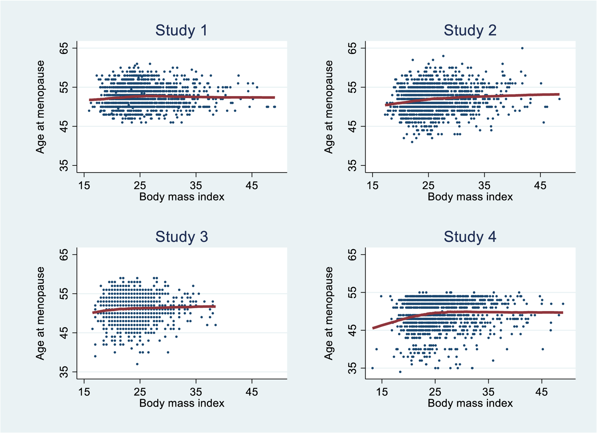
Scatter plots and lowess fits for age at natural menopause and baseline body mass index for the sample data set.

Table 1.

Summary statistics^* for the sample data set.

	Study 1	Study 2	Study 3	Study 4
Size of random sample, n	1500	1500	1500	1500
Age at natural menopause (years), mean (standard deviation)	52.55 (2.78)	51.93 (3.29)	51.18 (3.12)	49.38 (3.90)
Body Mass Index at baseline , mean (standard deviation)	25.44 (4.82)	26.16 (4.66)	23.58 (3.38)	25.82 (5.12)
Age at baseline (years), mean (standard deviation)	47.52 (1.43)	48.19 (4.05)	44.84 (3.44)	45.19 (5.19)
Smoking status at baseline, column %
Never	57.73	70.47	41.53	47.40
Former	28.13	20.00	39.60	28.47
Current	14.13	9.53	18.87	24.13
Education (years), column %
<=10	44.27	56.60	36.00	60.73
11–12	17.40	8.47	22.93	11.33
>12	38.33	34.93	41.07	27.93
Number of children, column %
0	7.87	14.93	8.73	16.60
1	8.87	7.67	15.87	15.00
2	40.67	37.40	44.60	45.53
>=3	42.60	40.00	30.80	22.87

^*There are small but statistically significant differences among the four studies (p < 0.0001 for all variables, based on one-way analysis of variance for the continuous variables and chi-squared tests for the categorical variables).

2.3. Modelling

The strategy is to model the association between the outcome and exposure of interest for each study separately (taking the covariates into account) and use each study-specific model to calculate estimates of the outcome. The individual study-specific estimates are then pooled pointwise using standard meta-analysis methods. Full details are provided in Appendix 1.

For the sample data we fitted multiple linear regression models for each study. The dependent variable was age at natural menopause. The independent variables were a curved function for BMI, a linear term for age at baseline, and indicator variables for the categories of smoking, level of education and number of children. The curved functions we used were fractional polynomials which are sums of polynomial and logarithmic terms [8] – see Appendix 1. For Study 1 the results obtained using the Stata command fp are: predicted age at natural menopause = 49.38 − 1134.30 × (1/BMI)² − 2.93 × ln(BMI) + 0.30 × baseline age + (0 if the participant was a never smoker, or 0.19 for a former smoker, or −0.09 for a current smoker) + and so on. Details of the study-specific models are shown in Table 2. The models differ in: the functional forms of terms for BMI, coefficients for the covariates and adequacy of fit as measured by adjusted R-squared values. Notably, the model for Study 1 has the poorest fit and the model for Study 4 has the best fit (as expected from the ceiling effect for age at natural menopause due to last available follow-up data for that study).

Table 2.

Models for age at natural menopause fitted to each data set separately: powers for fractional polynomials for BMI, coefficients and standard errors obtained using the Stata command fp.

	Study 1	Study 2	Study 3	Study 4
Powers for fractional polynomial for BMI	−2, 0	3, 3	−2, −2	−2, −2
First term for BMI	−1134.30 (555.94)	0. 00012 (0. 00015)	−4405.27 (3651.46)	−2736.25 (1579.61)
Second term for BMI	−2.93 (1.71)	−0. 00003 (0. 00004)	1689.89 (1380.56)	964.88 (588.62)
Age at baseline	0.30 (0.05)	0.55 (0.02)	0.58 (0.02)	0.65 (0.01)
Smoking status at baseline, column %
Never (reference)	0	0	0	0
Former	0.19 (0.16)	−0.01 (0.16)	−0.29 (0.14)	−0.23 (0.11)
Current	−0.09 (0.21)	−1.00 (0.21)	−0.80 (0.17)	−0.31 (0.12)
Education (years), column %
<=10 (reference)	0	0	0	0
11−12	0.10 (0.20)	0.10 (0.23)	0.27 (0.17)	0.22 (0.15)
>12	0.35 (0.16)	0.25 (0.14)	0.27 (0.14)	0.36 (0.11)
Number of children, column %
0 (reference)	0	0	0	0
1	−0.24 (0.35)	0.08 (0.27)	0.49 (0.26)	−0.15 (0.17)
2	0.13 (0.28)	0.17 (0.19)	0.46 (0.23)	0.09 (0.14)
>=3	−0.19 (0.28)	0.12 (0.19)	0.42 (0.24)	0.12 (0.15)
Constant	49.38 (6.88)	24.59 (0.82)	23.29 (1.55)	19.24 (0.66)
Adjusted R-squared	0.03	0.49	0.41	0.78

If the study-specific models all have the same terms (e.g., quadratic functions) an option for the meta-analysis is to calculate weighted averages of the parameter estimates from each study. If the study-specific models have different forms, an appropriate method is to calculate the predicted values of the outcome for each value of the exposure variable, and then calculate the weighted average across studies at each point, i.e., pointwise averaging. To ensure that each study contributes to the predicted values at every exposure value and covariate pattern, the study-specific model is used to calculated predicted outcome values and their standard errors for every participant in every study, not only the participants in the study used for the study-specific model (this approach is supported by the empirical studies by White et al. [7]).

Figure 2 shows lowess plots of the predicted values for age at natural menopause and their 95% confidence intervals (predicted value ± 1.96 × standard error) against BMI. Each plot depicts the whole dataset but using predictions derived from each of the four study-specific models (i.e. all 4 × 1500 sets of exposure and covariate values). Notably, consistent with the larger adjusted R-squared value, Study 4 shows less variability (i.e., narrower confidence intervals across the range of BMI values).

Figure 2.

Lowess plots of predicted values (and 95% confidence intervals) for age at natural menopause by body mass index for each study separately.

Standard meta-analysis methods are now used for the pointwise averaging. The standard errors of the predicted values are used to calculate the inverse variance weights with different formulas for fixed effects or random effects models (see Appendix 1). For a fixed effects model the exposure-outcome pattern is assumed to be the same for all the study populations and the variation in estimates is only due to sampling variation. For the random effects model, it is assumed that there are differences between the study populations and the goal is to estimate the average effect, therefore there is variation between the studies as well as sampling variation and so the confidence intervals are wider. Figure 3 shows lowess plots of the fixed effects and random effects weights for each study. Despite the identical sample size, there is considerable difference in the fixed effects weights over the range of BMI values and across the studies, with the largest weights usually for Study 4 which showed the most homogeneity (i.e., least variance) in Figure 2. In contrast, the random effects weights are very similar across the BMI range and for all studies. The meta-analysis is conducted pointwise (i.e., at each value of BMI observed within the whole dataset) with weighted averaging of the predicted values from each study. Note that the predicted values depend on the observed values of the exposure and the covariates for each participant. The meta-analysis results for fixed or random effects are shown in Figure 4. The pooled curves are similar for both methods of meta-analysis: low BMI was associated with early age at natural menopause, after adjusting for baseline age and other potential confounders. Age at natural menopause was highest for women with BMI around 30 and there was slight evidence of a decrease for more obese women. The confidence intervals are much wider for the random effects analysis, consistent with the underlying assumption of differences between the study populations.

Figure 3.

Lowess plots of the weights for each study that are used in the fixed effects and random effects meta-analyses.

Figure 4.

Results of meta-analysis of the association between age at natural menopause and body mass index: lowess plots for estimates and 95% confidence intervals.

3. Discussion

The goal of this paper is to make meta-analysis methods for exposure-outcome associations with IPD and continuous exposure data more accessible. While our approach follows that of Sauerbrei, Royston, White and colleagues [6, 7], a simplified version is used with the sample data set. Each step from the exploratory analysis to interpretation of the pooled results is explained.

In the example, the outcome is continuous and the curves of exposure-outcome association are estimated using multiple linear regression, including fractional polynomial terms. Other examples have involved time-to-event data and survival analysis [6, 7]. However, the method is just as applicable for counts or categorical outcomes (e.g., proportions) and a variety of generalized linear models (e.g., logistic regression). The strength of the method is that continuous curves are estimated for each study; that is, the exposure variable is not categorized.

To allow the curves to vary in shape, fractional polynomials were used in the example. But there are other functional forms that can be used such as ordinary polynomials, splines, generalized additive models, or even discontinuous forms. In the example, the number of terms and orders of the polynomials for the fractional polynomial were chosen using the default for the Stata command fp The Stata command fp uses forward selection of the numbers and powers of terms which are chosen to minimise the deviance. The R procedure mfp uses different criteria. It uses backward elimination and family-wise p-values; this procedure is designed to protect against overfitting. In the example the R command mfp produced simpler (linear) functions but very similar values for the predicted outcomes (see Appendix 2). More generally, the choice of form for the exposure-outcome curve may be made using subject-matter knowledge, visual inspection of the curves, and comparisons of alternative forms (e.g., using criteria for model fit such as AIC or BIC). For any curve fitting there is a tension between selecting forms that are too simple (e.g., linear only) and overfitting with more complex ones.

In some cases, selecting the same form of curve for all studies may be appropriate. In this situation meta-analysis could be used to average the parameter estimates rather than pointwise pooling of the curves [11]. For meta-analyses of large numbers of studies with many participants this approach would be less computationally intensive, and White et al. have shown that the results are likely to be similar [7]. This strategy is also likely to have more power to model complicated curves [12]. Software for pooling parameter estimates is available in Stata and R programs both called mvmeta [7, 12].

A notable difference between the method used above and the approach described by Sauerbrei, Royston, White and others [6, 7] and implemented in the Stata program metacurve [13], is their use of an intermediate stage of fitting ‘confounder models’. Instead of fitting a study-specific model with the outcome as the dependent variable and fractional polynomial terms of the exposure and covariates as the independent variables, they first fit a ‘confounder model’ which has the exposure as the dependent variable and the covariates as the independent variables. Next the linear predictor of this model is calculated for all individuals, this is called the ‘confounder index’. Finally, they fit a study-specific model with the outcome as the dependent variable and the fractional polynomial of the exposure, adjusted for the confounder index. An advantage of using a confounder model is that it can accommodate more complex terms for the covariates. For instance, in the example above the covariate, baseline age, was treated as a linear term, but in a confounder model a fractional polynomial, or other functional form, for this variable could have been included. A non-statistical researcher may initially find the concept of a confounder model confusing because the main exposure has the role of the dependent variable. This is why confounder models were not used in the example, but when they were used the final results were the same. A confounder model is analogous to a propensity score [14] with a model fitted for the exposure variable rather than the outcome but the coefficients may be less easily interpreted.

In the example, for simplicity, centring and scaling were not used for any of the continuous variables. Nevertheless, it is usually better statistical practice to standardize the exposure and other covariates, at least by centring them, as this can help interpretation of the estimates and reduce collinearity. In some situations, it is important that the results can be readily transformed back to the original scales (as in the example of age at natural menopause and BMI). In other situations, effect sizes relative to some fixed value are more interpretable, e.g., risk of an outcome relative to a reference level of the exposure [7, 12].

Using IPD to fit a continuous curve for the exposure-outcome association is preferable to categorizing the exposure. Categorizing continuous variables reduces the precision and power of an analysis [5]. If only published aggregate results, not IPD, are available for a continuous exposure variable, the effect estimates usually refer to categories of exposure, and these may be used to estimate the underlying continuous association [15]. Meta-analysis of these data is complicated by the correlation of estimates from the same study across the exposure range. Specialised software includes the SAS macro metadose [16] and the R program dosresmeta [17].

As with any meta-analysis it is important to consider whether the studies and their results are sufficiently similar to justify averaging them. Factors to be considered include differences in: study design, covariates measured, measurement scales, and ranges of exposure and outcome measures [18, 19]. Recommendations for exploring heterogeneity for IPD include comparisons across studies of the distributions and associations between variables [19, 20]. For the InterLACE consortium from which the example data were drawn [9], some studies collected age at menopause retrospectively and other prospectively, for some BMI was calculated from self-reported measures while others provided measured weight and height. Nevertheless, visual inspection of the plots in Figure 1 and summary statistics in Table 1 suggest sufficient similarity in the sample data to justify meta-analysis.

The goal of making the sample data set publicly available, providing segments of Stata and R code, and output, is to facilitate replication of the results, comparison or alternative methods and software, and extension to other situations.

Highlights.

• Methods for meta-analysis of studies with individual participant data and continuous exposure variables are well described in the statistical literature but are not widely used in clinical and epidemiological research.

• The purpose of this paper is to make the methods more accessible.

• In a two-stage process, response curves for each study are estimated separately and then pointwise weighted averages are calculated using fixed effects or random effects methods.

• A sample data set, segments of Stata and R code, and outputs are provided to enable replication and facilitate adaptation to other settings.

Appendix 1. Mathematical methods

Notation.

The data are denoted by y_jk, z_jk and c_jkl, where y is the outcome or response variable, z is the exposure or dose variable of interest, and c denotes the covariates; j = 1, …, J denotes the studies, k = 1, …, K_j denotes the observations in each study, and l denotes the covariates (l = 1, …, L). For the sample data there are J = 4 studies with K = 1500 observations for each study and L = 4 covariates.

Fractional polynomials.

A fractional polynomial of a variable x is defined as $f\left(x\right)={\beta }_0+{\sum }_{m=1}^M{\beta }_m{x}^{p_m}$ with degree M, the number of terms, and powers p_m [8]. Usually, M = 2 and the values p_m are selected from −2, −1, −0.5, 0, 0.5, 1, 2 and 3; x⁰ is defined to be ln(x) and if a power p is repeated the terms are x^p + x^pln(x).

Fitting models for each study separately.

For the sample data we fitted models $f\left(y_{jk}\right)={\beta }_0+{\sum }_{m=1}^M{\beta }_m{z}_{jk}^{p_m}+{\sum }_{l=1}^L{\gamma }_{jkl}{c}_{jkl}$ for each study separately using multivariable linear regression. The fractional polynomial and covariate terms were all fitted at the same time (using the Stata command fp. The powers p₁ and p₂ for each study were selected based on the model with the lowest deviance (the default method in Stata). The continuous covariate baseline age was fitted as a linear term. In this case, for simplicity, none of the variables was transformed (e.g., centred or scaled).

Predicted values and standard errors of predicted values.

For each model predicted values and their standard errors need to be calculated for every participant, not only those in that particular study. To do this it may be convenient to work with the data in “long form”, that is with the observations of Study 1 stacked on those for Study 2, and so on. We use the index i for each of the J × K rows and retain the index j for studies. With this change in notation, each row includes the predicted values ψ_ij and their standard errors s_ij for each of the J studies. Figure 2 shows the J × K predicted values and their 95% confidence intervals (ψ_ij ± 1.96 s_ij) plotted for each study separately.

Meta-analysis.

Standard meta-analysis methods are now used to average the predicted values ψ_ij across each row using inverse variance weights calculated from the standard errors s_ij. Using similar notation to Sauerbrei and Royston [6], let $v_{ij}=s_{ij}^2$ and $R_i={\sum }_{j=1}^J\left(1/v_{ij}\right)$ For the fixed effects estimate, the weights are given by w_ij = 1/(v_ijR_i) and the estimate is

$${\psi }_i^{FE}={\sum }_{j=1}^J{w}_{ij}{\psi }_{ij},\text{ with variance given by }{\mathit{\text{var}}}_i^{FE}=1/R_i$$

for row i of the stacked data. For the random effects estimate, first calculate $Q_i={\sum }_{j=1}^J\left[{\left({\psi }_{ij}-{\psi }_i^{FE}\right)}^2/v_{ij}\right]$, $D_i=R_i-\left[{\sum }_{j=1}^J\left(1/v_{ij}^2\right)/R_i\right]$, ${\tau }_i^2=\mathit{\text{max}}\left\{0,\left[Q_i-(J-1)\right]/\left(R_i-D_i\right)\right\}$ and $W_i={\sum }_{j=1}^{J}1/\left(v_{ij}+{\tau }_i^2\right)$. Then the weights are given by $u_{ij}=1/\left\{\left(v_{ij}+{\tau }_i^2\right)W_i\right\}$ and the random effects estimate is

$${\psi }_i^{RE}={\sum }_{j=1}^J{u}_{ij}{\psi }_{ij}\text{, with variance given by }{\mathit{\text{var}}}_i^{RE}=1/W_i\text{.}$$

Figure 3 shows the fixed effects weights w_ij and the random effects weights u_ij for each study, plotted for all i and Figure 4 shows the results of the meta-analysis using either fixed or random effects analysis.

Appendix 2. Segments of Stata and R code and output.

References

- 1.Greenland S, Longnecker MP. Methods for trend estimation from summarized dose–response data, with applications to meta-analysis. American Journal of Epidemiology 1992; 135: 1301–1309 [DOI] [PubMed] [Google Scholar]
- 2.Liu Q, Cook NR, Bergström A, Hsieh CC. A two-stage hierarchical regression model for meta-analysis of epidemiologic nonlinear dose–response data. Computational Statistics & Data Analysis 2009; 53: 4157–4167, [Google Scholar]
- 3.Rota M, Bellocco R, Scotti L, Tramacere I, Jenab M, Corrao G, La Vecchia C, Boffetta P, Bagnardi V. (2010), Random-effects meta-regression models for studying nonlinear dose–response relationship, with an application to alcohol and esophageal squamous cell carcinoma. Statist. Med 2010; 29: 2679–2687. doi: 10.1002/sim.4041 [DOI] [PubMed] [Google Scholar]
- 4.Debray TP, Moons KG, van Valkenhoef G, et al. Get real in individual participant data (IPD) meta-analysis: a review of the methodology. Res Synth Methods. 2015; 6: 293–309. doi: 10.1002/jrsm.1160 [DOI] [PMC free article] [PubMed] [Google Scholar]
- 5.Royston P, Altman DG, Sauerbrei W. Dichotomizing continuous predictors in multiple regression: a bad idea Statist. Med 2006; 25:127–141 [DOI] [PubMed] [Google Scholar]
- 6.Sauerbrei W, Royston P. A new strategy for meta-analysis of continuous covariates in observational studies. Statist. Med 2011; 30: 3341–60. [DOI] [PubMed] [Google Scholar]
- 7.White IR, Kaptoge S, Royston P, Sauerbrei W. Meta-analysis of non-linear exposure-outcome relationships using individual participant data: A comparison of two methods. Statist. Med 2019; 38: 326–38. [DOI] [PMC free article] [PubMed] [Google Scholar]
- 8.Royston P, Altman DG. Regression using fractional polynomials of continuous covariates: parsimonious parametric modelling. Journal of the Royal Statistical Society. Series C (Applied Statistics) 1994; 43: 429–467 [Google Scholar]
- 9.Mishra GD, Anderson D, Schoenaker DAJM, Adami H-O, Avis NE, Brown D, et al. InterLACE: A new International Collaboration for a Life Course Approach to Women’s Reproductive Health and Chronic Disease Events. Maturitas 2013; 74: 235–40. [DOI] [PubMed] [Google Scholar]
- 10.Zhu D, Chung HS, Pandeya N, Dobson AJ, Kuh D, Crawford SL, Gold EB, Avis NE, Giles GG, Bruinsma F, Adami HO, Weiderpass E, Greenwood DC, Cade JE, Mitchell ES, Woods NF, Brunner EJ, Simonsen MK, Mishra GD. Body mass index and age at natural menopause: an international pooled analysis of 11 prospective women’s health studies. Eur J Epidemiol. 2018; 33: 699–710. [DOI] [PubMed] [Google Scholar]
- 11.Burke DL, Ensor J, Riley RD. Meta-analysis using individual participant data: one-stage and two-stage approaches, and why they may differ. Statist Med. 2017;36(5):855–75. [DOI] [PMC free article] [PubMed] [Google Scholar]
- 12.Gasparrini A, Armstrong B, Kenward MG. Multivariate meta-analysis for non-linear and other multi-parameter associations. Statist. Med 2012; 31: 3821–39. [DOI] [PMC free article] [PubMed] [Google Scholar]
- 13.White IR. Multivariate random-effects meta-analysis. Stata J. 2009; 9: 40–56. [Google Scholar]
- 14.Austin PC. A tutorial and case study in propensity score analysis: an application to estimating the effect of in-hospital smoking cessation counseling on mortality. MultivarBehav Res. 2011;46(1):119–151. [DOI] [PMC free article] [PubMed] [Google Scholar]
- 15.Bagnardi V, Zambon A, Quatto P, Corrao G. Flexible meta-regression functions for modeling aggregate dose-response data, with an application to alcohol and mortality, Am J Epidemiol,2004; 159: 1077–1086. [DOI] [PubMed] [Google Scholar]
- 16.Li R, Spiegelman D (2010). “The SAS %metadose Macro.” http://www.hsph.harvard.edu/donna-spiegelman/software/metadose/.
- 17.Crippa A, Orsini N. Multivariate dose–response meta-analysis: the dosresmeta R package. J Stat Software 2016; 72: 1–15. [Google Scholar]
- 18.Cordero CP, Dans AL. Key concepts in clinical epidemiology: detecting and dealing with heterogeneity in meta-analyses. J Clin Epidemiol. 2021; 130: 149–51. [DOI] [PubMed] [Google Scholar]
- 19.Smith CT, Williamson PR, Marson A. Investigating heterogeneity in an individual patient data meta-analysis of time to event outcomes. Statist. Med 2005, 24: 1307–1319. [DOI] [PubMed] [Google Scholar]
- 20.Steyerberg EW, Nieboer D, Debray TPA, van Houwelingen HC. Assessment of heterogeneity in an individual participant data meta-analysis of prediction models: An overview and illustration. Statist. Med 2019; 38: 4290–4309. [DOI] [PMC free article] [PubMed] [Google Scholar]
Associated Data
This section collects any data citations, data availability statements, or supplementary materials included in this article.