Real-time deep learning assisted skin layer delineation in dermal optical coherence tomography

Abstract

We present deep learning assisted optical coherence tomography (OCT) imaging for quantitative tissue characterization and differentiation in dermatology. We utilize a manually scanned single fiber OCT (sfOCT) instrument to acquire OCT images from the skin. The focus of this study is to train a U-Net for automatic skin layer delineation. We demonstrate that U-Net allows quantitative assessment of epidermal thickness automatically. U-Net segmentation achieves high accuracy for epidermal thickness estimation for normal skin and leads to a clear differentiation between normal skin and skin lesions. Our results suggest that a single fiber OCT instrument with AI assisted skin delineation capability has the potential to become a cost-effective tool in clinical dermatology, for diagnosis and tumor margin detection.

1. Introduction

We present deep learning assisted optical coherence tomography (OCT) imaging for quantitative tissue characterization and differentiation in dermatology.

OCT is a cross-sectional imaging modality widely used in many fields of biomedicine [1]. With its capability to delineate retinal layers and other ocular structures through non-invasive imaging, OCT has been widely adopted in clinical ophthalmology [2,3]. OCT is also a promising non-invasive imaging technique for dermatology, because it provides sufficient imaging depth (up to several millimeters) and spatial resolution (1μm to 10μm) to profile subsurface skin layers of interest [4]. OCT can be used to image the altered skin anatomy due to skin pathology. Researchers assessed the potential of OCT in the diagnosis of non-melanoma skin cancers (NMSCs) and benign skin lesions. OCT image features for NMSCs have been identified and reported in literature. These features include dark lobules with or without a border, white streaks and dots in the epidermis, and loss of the normal layered skin architecture [5–7]. Previous studies also investigated OCT’s capability in differentiating cancerous skin from normal skin, and used it to assist in surgical removal of skin lesions [8]. Moreover, the thickness of the epidermis and the characteristics of dermal-epidermal junction (DEJ) identified by OCT can be correlated with a variety of skin conditions [9,10]. Knowledge on epidermal thickness and DEJ condition is critical in clinical practices.

However, the use of OCT in clinical dermatology remains limited for several reasons. First, the conventional OCT imaging system relies on a bulky sample arm for image acquisition, making it more cumbersome than a handheld dermoscope with wide clinical adoption. Second, it is challenging to identify individual skin layers through visual inspection because OCT images are overwhelmingly affected by speckle noise [11]. As to histopathology, it is critical to identify the disruption of normal layer structures of the skin in OCT images. Third, current high-speed OCT engines acquire data at a speed prohibitively fast (~100 kHz Ascan rate) for real-time visual inspection. Analysis of OCT images relying on manual annotation and post-processing is time and labor intensive.

To extract information from massive OCT data and use OCT imaging to guide clinical procedures in dermatology, it is desirable to have a platform that allows real-time OCT imaging and high-level information extraction. In this manuscript, we describe innovative solutions in instrumentation and signal processing to advance the application of OCT in clinical dermatology. We have demonstrated a manually scanned single fiber OCT (sfOCT) instrument that acquires OCT images from the skin. The focus of this study is to implement an artificial intelligence (AI) approach to automatically segment OCT images of the skin into different anatomical layers. Our OCT imaging is based on a common path single fiber probe that does not rely on a mechanical beam scanner for form 2D images [12,13]. The probe acquires 2D OCT images through manual scanning, and performs speckle decorrelation analysis to correct distortion artifacts due to nonconstant scanning speed [14,15]. Compared to all the other OCT technologies utilized in dermatology, our sfOCT system has the simplest imaging probe and scanning mechanism, to the best of our knowledge. On the other hand, the AI algorithm functionalizes the imaging instrument and extracts clinically relevant information from image data. We use U-Net to segment OCT images of the skin into different layers (stratum corneum, epidermis, and dermis). Convolutional neural networks (CNN) and other deep learning algorithms have been developed for biomedical image analysis. U-Net, a widely used CNN architecture for semantic image segmentation [16], has been adopted by the OCT community to segment images of the retina and the skin [17–20]. For skin layer characterization, we use a U-Net to functionalize a single fiber OCT instrument for in vivo, real-time imaging, which, to the best of our knowledge, is unprecedented. In addition, we demonstrate the integration of data acquisition, image reconstruction and AI analysis in real-time software, which has the potential to significantly advance the clinical application of OCT in dermatology.

In particular, a valuable application for our technology in clinical dermatology involves a form of dermatologic surgery called Mohs micrographic surgery (MMS) [21]. On cosmetically sensitive areas such as the head and neck, a dermatologic surgeon can use MMS to conduct a stepwise removal of a biopsy-proven NMSC, checking histopathological tissue sections for microscopic margin clearance after each subsequent stage. With AI functionalized sfOCT, the tumor margin can be determined in real time through automatic skin layer delineation and abnormality detection. This will increase the precision of the first excision and potentially decrease the number of stages required to achieve complete removal of the tumor. By harnessing AI to assist in determining the presence or absence of a tumor, sfOCT becomes more accessible to all Mohs surgeons, regardless of OCT experience.

This manuscript is organized as the follows. First, we describe the OCT imaging system used, single fiber imaging probe, and the architecture of our U-Net. Afterwards, we describe the imaging experiments. We then represent results on the performance of U-Net, quantitative evaluation of epidermal thickness of normal skin, and U-Net analysis of skin lesions. Our results suggest that a single fiber OCT instrument functionalized with an AI algorithm has the potential to become a cost-effective tool in clinical dermatology, for diagnosis and tumor margin delineation.

2. Method

2.1. OCT imaging based on a handheld single fiber probe

We used a swept source OCT engine (AXSUN OCT engine, 1060 nm central wavelength, 100 nm bandwidth) for imaging with a 100 kHz Ascan rate. The imaging capability of the swept source OCT engine was described in our previous publication [22]. Briefly, the output of the swept source is routed by a fiber optic circulator to a single fiber probe. Reference and sample light derived from the probe is routed back to the OCT engine for detection. We make the imaging probe (Fig. 1(a)) by extending an FC/APC fiber patch cord with a spliced segment of bare fiber. We integrate the distal tip of the fiber with a stainless steel needle for rigidity, and attached the fiber-optic probe to a plastic handle. We cleave the fiber tip to generate a flat surface (the inset at the bottom left of Fig. 1(a)) that provides a reference light (E_r). The fiber-optic probe collects signal photons from the sample (E_s) that interfere with reference light (E_r) to create depth resolved profiles of the sample, in a common path interferometer [12,13]. Notably, the needle used to house the fiber optic probe is a feed needle (20 gauge, Roboz Surgical Instrument) with a rubber cap at the tip. The rubber cap ensures a relatively constant pressure between the probe and the skin, and minimizes the deformation of skin layers during scanning. The axial resolution was measured to be 6μm. With a bare fiber probe, the lateral resolution decreases as the imaging depth and was measured to be 35μm at an imaging depth of 1.1 mm. To characterize the lateral resolution of the fiber probe, we scanned the probe across a specular sample that has a step function reflectivity profile in lateral dimension. The resultant lateral profile could be modeled as an erfc function, assuming the lateral PSF of the OCT system with a bare fiber probe to be Gaussian. Through a non-linear least square fitting, we extracted the full width maximum of Gaussian PSF and estimated the lateral resolution to be 35 μm at the depth of 1.1 mm.

Fig. 1.

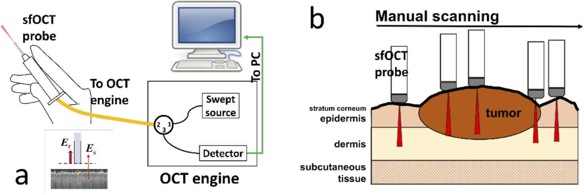
(a) Swept source OCT system that has a manually scanned single fiber probe; (b) sfOCT probe is manually scanned across a region of interest to generate a 2D image.

Unlike a conventional OCT imaging system, the single fiber OCT (sfOCT) probe acquires 2D images through manual scanning (Fig. 1(b)). Such a unique scanning mechanism allows the acquisition of 2D skin images with a probe that is lightweight, low cost and disposable. Notably, OCT signals directly obtained from manual scanning suffer from distortion artifacts, because the probe is manually scanned at a nonconstant transverse speed. To correct the distortion artifact, we utilize a motion tracking method based on speckle decorrelation analysis, to quantify the lateral displacement between adjacent Ascans and correct distortion artifact [14,15]. Briefly, we calculate the cross-correlation ρ_i between sequentially acquired Ascans $\left(S_i\text{and }{S}_{i+1}\right):{\rho }_i=\frac{\left(S_i-S_i\right)\left(S_{i+1}-S_{i+1}\right)}{{\sigma }_i{\sigma }_{i+1}}$, use the cross-correlation coefficient to quantify lateral displacement: $\delta x_i=w_0\sqrt{ln\left(\frac{1}{{\rho }_i}\right)}$, calculate the accumulated lateral displacement $x_n=\sum _{i=1}^n\delta x_i$, and sample an Ascan when x_n reaches Δx that is the pre-determined lateral sampling interval. Δx was chosen to be 17μm in our imaging experiments to satisfy Nyquist sampling given a lateral resolution of 35μm, unless otherwise stated. With the above motion tracking and Ascan resampling method, we are able to reconstruct distortion-free OCT images using data obtained from manual scanning. The system acquires OCT signal using a frame grabber (PCIe-1433, National Instrument), processes signal in real-time using a GPU (NVIDIA gtx1080), and uses a Dell Precision workstation to coordinate data acquisition, processing, and display. The data set for training was obtained using software develop in house in C++. The software uses CUDA for real-time OCT signal reconstruction, distortion correction and display. For real-time U-Net delineation of the skin, we implemented OCT data acquisition, image reconstruction, distortion correction, and U-Net segmentation (semantic segmentation) using Matlab 2019.

2.2. U-Net that segments OCT images of the skin

In this study, we use a neural network with U-Net architecture to generate the rules to assign a label (air, stratum corneum, epidermis, or dermis) to every pixel of an OCT image. The network is trained using image data (OCT images, Fig. 2(a)) and ground truth pixel classification (expert manual segmentation, Fig. 2(b)), to predict pixel category (Fig. 2(c)). Scale bars represent 500μm. The architecture of U-Net used in this study is illustrated in Fig. 3. The U-Net has a contracting encoder branch and an expanding decoder branch. The encoder branch has 5 stages to extract multiscale features of the input image while the decoder branch has 5 stages to generate a spatially resolved prediction of individual pixels for segmentation. As illustrated in Fig. 3, each encoder stage has 5 layers (3×3 convolution layer, ReLU activation layer, 3×3 convolution layer, ReLU activation layer, and max pooling layer). Each decoder stage consists of 7 layers (up convolution layer for upsampling, up ReLU layer, concatenation layer, 3×3 convolution layer, ReLU layer, 3×3 convolution layer, and ReLU layer). The 1^st, 2^nd, 3^rd, 4^th and 5^th encode stage generate 32, 64, 128, 256, 512 features, respectively. For each pixel, the U-Net effectively calculates its likelihood to be a specific category. The pixel is assigned a category that corresponds to the highest probability. In this study, we design the U-net to have input and output images with a dimension of 256 (axial dimension or z dimension) × 32 (lateral dimension or × dimension). Batch normalization is not implemented, because the U-Net takes log scale OCT data with compressed amplitude as the input and the amplitude of OCT signal is directly related to the optical properties of the sample (absorption coefficients and scattering coefficients). Cross entropy is used as the loss function for training. The U-Net is trained using experimental data iteratively to achieve satisfactory accuracy, and evaluated using a k fold cross validation strategy. The OCT engine takes 1024 sampling points in spectral domain, resulting in 513 effective pixels in each Ascan due to complex conjugation symmetry after Fourier transform. To segment a 2D image that has more than 32 Ascans using our U-Net, the image is first cropped to include 256 pixels in axial (depth) dimension and divided into multiple patches each with 32 Ascans in lateral dimension. We utilize the first 256 pixels in an Ascan for U-Net segmentation. These pixels provide an imaging depth of 1.4 mm, which is sufficient to reveal most pathologies within the epidermis and dermis. OCT pixels at a larger imaging depth are extremely noisy and provide limited information with clinical significance. In lateral dimension, the image input into the U-Net has 32 Ascans. The use of small image patches for segmentation is critical for real-time imaging studies, because the OCT system can acquire a small amount of Ascans in a short period of time and present the results of U-Net segmentation with a minimal latency. Moreover, the small dimension is critical for efficient network training with GPU. To improve the quality of segmentation and generate areas with connected pixels belonging to the same class, we further filter the output of U-net segmentation. Consider a small square region centered at pixel (i,j) with N×N pixels. The algorithm evaluates the prediction of U-net for pixels within this region, determines the most populous category, and assigns this category to pixel (i,j). Compared to morphological opening operation that serves a similar purpose, our method is robust at the geometric boundary between different skin layers, where the predicted pixel category has large uncertainty. Using the results of U-Net segmentation, we are able to determine the dermo-epidermal junction (DEJ) that is of clinical significance, by detecting the pixel at which the label turns from epidermis to dermis in each Ascan.

Fig. 2.

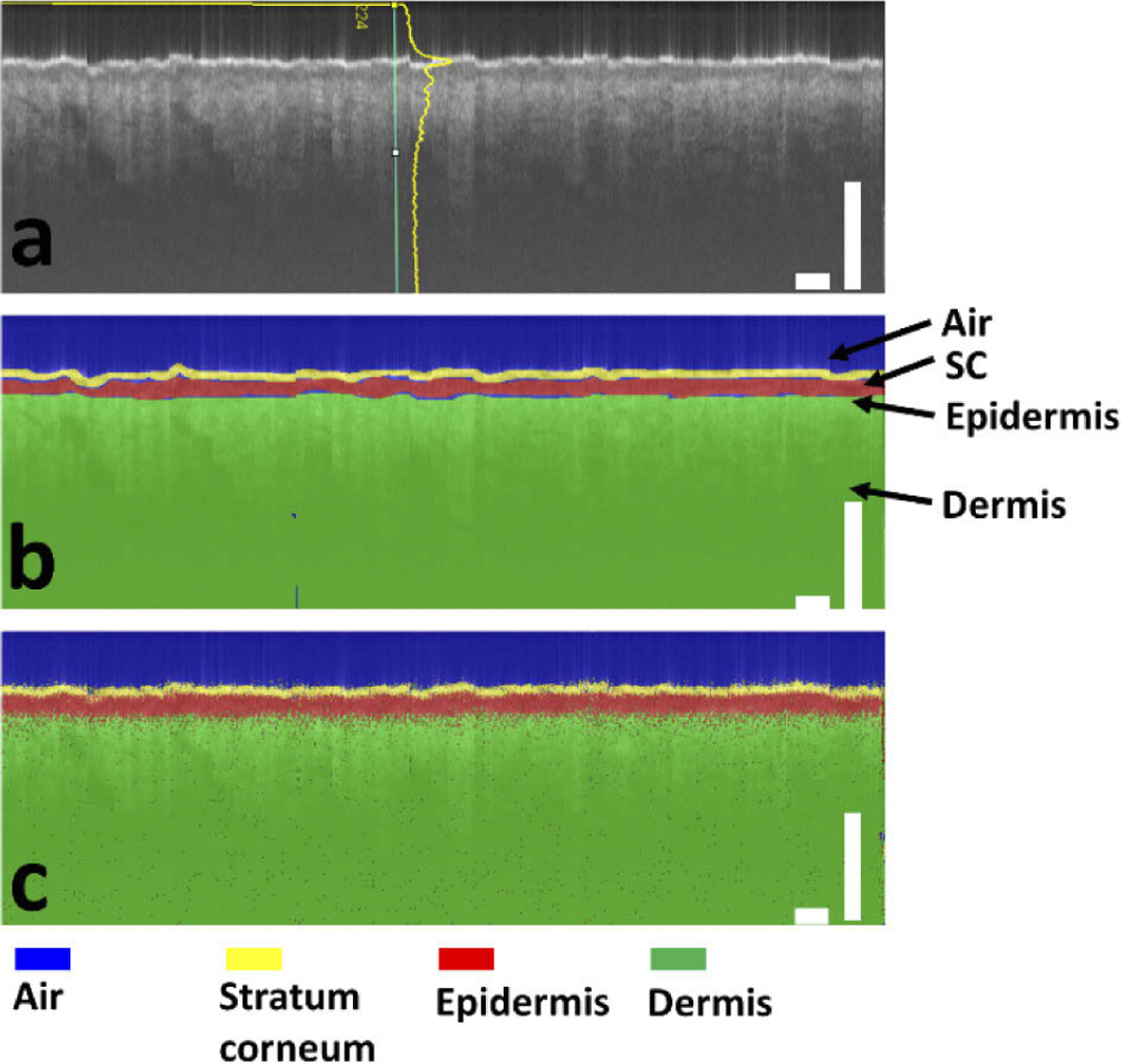
(a) OCT image and (b) manually labeled layers of air (blue), stratum corneum (SC) (yellow), epidermis (red), and dermis (green) for U-Net training; (c) U-net generates labels for individual pixels of the OCT image. Scale bars represent 500μm.

Fig. 3.

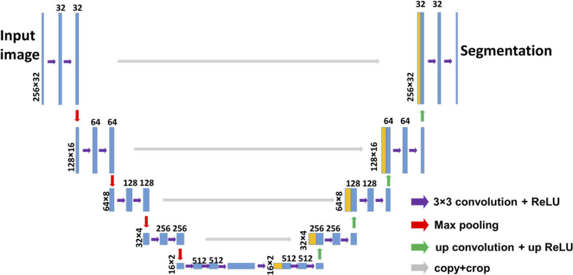
U-Net architecture for dermal OCT image segmentation.

2.3. Imaging experiments

We trained the U-Net using data obtained from 5 healthy subjects (Table 1). For each subject, OCT images were obtained from three body sites (volar forearm, dorsal forearm, and forehead), by manually scanning the sfOCT probe on top of the skin. Furthermore, using U-Net trained with OCT images of healthy skin, we validated AI functionalized OCT imaging on skin lesions, including scar tissue and a skin tumor. For scar tissue characterization, we imaged an area of forearm skin that had been treated with CO₂ fractional laser seven days prior, leaving behind immature scars. We also evaluated OCT imaging and U-Net segmentation of skin tumors. We performed manually scanned OCT imaging on patients who were scheduled to receive MMS for a biopsy-proven BCC or SCC tumor. Patients were recruited at a private dermatology practice under institutional review board (Advarra) approved protocol, along with written informed consent and HIPAA authorization.

Table 1.

Information on healthy subjects who participated the imaging study.

	Age	Sex	Skin type
subject 1	29	F	3
subject 2	30	F	2
subject 3	25	F	1
subject 4	37	F	3
subject 5	30	M	3

3. Results

3.1. U-Net training and validation

We trained the U-Net with 15 manual scans obtained from 5 healthy subjects. Each manual scan was a 2D image with a dimension of 512 (axial) by 1024 (lateral). The ground truth pixel classification was generated by manual annotation, as illustrated in Fig. 2(b). We cropped the OCT images and the corresponding labeling in axial dimension, divided each 2D image into multiple patches, and obtained 240 patches for U-Net training. Each patch had a dimension of 256 (axial) by 32 (lateral). To improve the robustness of the segmentation algorithm, we also included additional OCT images obtained from one of the subjects, with imaging probes located at different axial offsets from the surface of the skin. The image dataset thus had 348 patches, all from healthy subjects. The U-Net was trained in Matlab 2019b, on graphic processing units (GPU-GTX1070). The training was accomplished in approximately 10 minutes with a mini batch size of 10, initial learning rate of 10⁻⁴, iterated for 50 epochs. To validate the segmentation of the U-Net with architecture shown in Fig. 3, we adopted a K-fold (K=5) cross validation strategy. In each fold, we shuffled image patches randomly and divided them into non-overlapping partitions for training, validation, and test data sets at a ratio of (K-2):1:1. In the random partitioning, image patches from the same subject may be found in training, validation and testing set. The accuracy was quantified by correlating the U-Net predicted pixel category with the ground truth category. The overall accuracy of the K-fold cross validation had a mean value of 0.96. Using the testing data set, we calculated the dice similarity coefficients (DSC) between U-net prediction and the ground truth for different pixel classes: DSC=|X_U−Net∩X_gt|/(X_U−Net|+|X_gt|). Here X_U−Net represents pixels classified into a specific category by U-Net, X_gt represents pixels classified into a specific category in ground truth (manual annotation), ∩ represents intersection between sets X_U−Net and X_gt, and ∥ represents to calculate the cardinality for a set (number of elements in the set). Notably, the layer of stratum corneum had a much smaller number of pixels compared to other categories, so we grouped pixels of stratum corneum and epidermis for DSC calculation. Figure 4 shows the mean DSC for each pixel category in the 5-fold validation and the error bars show the standard deviation of the accuracy assessments. Mean DSC values are 0.9791, 0.9601 and 0.8361, for pixels corresponding to air, dermis, and combined stratum corneum (SC) + epidermis, respectively. Results in Fig. 4 suggest a satisfactory performance of U-Net skin layer delineation.

Fig. 4.

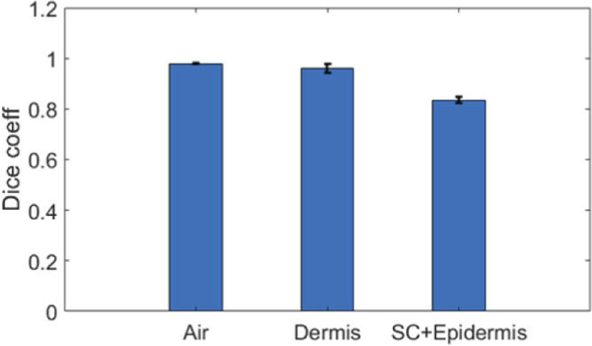
Dice similarity coefficients between U-Net prediction and ground truth labeling for air, dermis, and combined stratum corneum (SC) and epidermis.

3.2. Real-time OCT imaging and skin delineation based on U-Net

Figure 5(a) illustrates the graphic interface of our AI assisted real-time imaging platform. In our previous publications, we reported real-time, manually scanned OCT imaging, using in-house developed software (C++ with CUDA) to perform parallel GPU computation [14,15]. In this study, we further demonstrated real-time imaging and AI segmentation capability, using software developed in Matlab with its deep learning tool box (for semantic segmentation using U-Net) and parallel computation tool box (for parallel computation using GPU). The top panel of the graphic interface shows and updates OCT data obtained during manual scanning. Through speckle decorrelation analysis, the software tracks lateral scanning speed and updates the OCT image accordingly. The bottom panel of the graphic interface shows the results of U-Net segmentation overlaid with OCT image. Figure 5(b) shows the flow chart of the software. After a batch of spectral data (1024 spectral interferograms) is acquired, OCT signal is reconstructed through FFT. Afterwards, speckle decorrelation analysis is performed to re-sample the Ascans and assemble a distortion free 2D image. The software then uses the pre-trained U-Net to segment the newly acquired image and update the display and segmentation results. Based on the results of U-Net segmentation, the software counts the number pixels (N_ep) classified as epidermis in each Ascan, and quantifies epidermal thickness T_ep: T_ep=N_epδd where δd is the depth sampling interval. Using 32 Ascans that are assembled into the image most recently, the software updates the estimation of epidermal thickness for the skin currently under OCT imaging. Visualization 1, Visualization 2, and Visualization 3 show real-time display of OCT imaging and U-Net segmentation, when the single fiber OCT probe was scanned at the volar forearm, dorsal forearm, and forehead of a healthy subject.

Fig. 5.

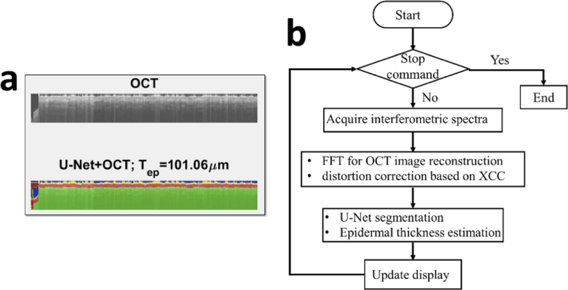
(a) graphic interface of AI assisted OCT imaging; (b) flow chart for signal processing.

3.3. Quantitative assessment of epidermal thickness in healthy skin based on U-Net delineation

The thickness of epidermis is a critical parameter in clinical dermatology, as many pathologies are related to disruption of DEJ. Here we demonstrate the capability of U-Net in assessing epidermal thickness of healthy skin. Figure 6 shows results obtained from the same subject, at different anatomical sites. Scale bars represent 500μm. Results in the first column (Fig. 6(a) – (c)) show an OCT image obtained from the volar forearm (skin site 1) of the subject, U-Net delineation overlaid with OCT image, and DEJ detected (red line in Fig. 6(c)). Results in the second column (Fig. 6(d) – (f)) were obtained from the dorsal forearm (skin site 2), and results in the third column (Fig. 6(g) – (i)) were obtained from the forehead (skin site 3). In Fig. 6, the segmentation of skin layers and the detected DEJ are consistent with known features of skin OCT images. The most superficial layer, which is thin and bright, is recognized as stratum corneum, followed by the epidermis which is less scattering, and the dermis which is slightly brighter at the beginning and decreases due to light absorption and scattering [23]. To illustrate the difference in epidermal thickness at different body sites, Fig. 7(a) shows epidermal thickness along × (lateral) dimension for volar forearm (skin site 1), dorsal forearm (skin site 2), and forehead (skin site 3). On average, the epidermis at the forehead had a larger thickness compared to the epidermis at the forearm, which is consistent with published results [24]. To further demonstrate this, we selected sub-regions from the upper left corner of Fig. 6(a), (d), and (g), and show them in Fig. 7(b), (c), and (d). The difference in epidermal thickness can be clearly visualized, as indicated by the red arrows.

Fig. 6.

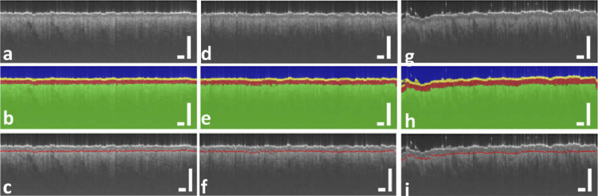
(a), (d), and (g): OCT image obtained from volar forearm (skin site 1), dorsal forearm (skin site 2), and forehead (skin site 3); (b), (e), and (h): U-Net segmentation corresponding to (a), (d), and (g); (c), (f), and (i): DEJ detected and shown as red lines. Scale bars represent 500μm.

Fig. 7.

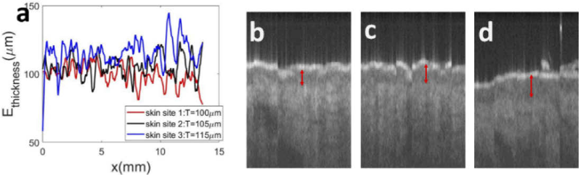
(a) Epidermal thickness calculated based on the results of U-net segmentation for skin sites 1, 2, and 3, corresponding to images shown in Fig. 6 (a), (d), and (g); (b)-(d): sub-regions of OCT images that highlight the difference in epidermal thickness. Red arrows indicate the thickness of epidermis.

We summarize U-Net assessment of epidermal thickness of healthy subjects in Table 2. For ground truth epidermal thickness, we counted the number of pixels classified as epidermis in manual annotation in each Ascan. Afterwards, we determined the epidermal thickness in each Ascan and the average epidermal thickness in the entire 2D image. For epidermal thickness evaluated based on U-Net segmentation, we counted the number of pixels classified as epidermis according to the output of the U-Net. In addition, we performed two sets of manual measurement (Manual 1 and Manual 2 in Table 2) of epidermal thickness on all the images in our data set. Two individuals (N.C. and Y.L) used the distance measurement tool in ImageJ to measure the thickness of epidermis at discrete locations. For each 2D image, a measurement was taken for every 64 Ascans and these measurements were averaged to assess the epidermal thickness.

Table 2.

Epidermal thickness at skin sites 1, 2, and 3 of 5 healthy subjects evaluated based on ground truth annotation, U-Net segmentation, and discrete manual measurement by two individuals.

		Ground truth (μm)	U-Net(μm)	Manual1(μm)	Manual2(μm)
Subject 1	Site 1	121.56	105.81	147.92	96.69
	Site 2	98.42	104.31	109.05	110.47
	Site 3	128.74	116.37	153.26	115.95
Subject 2	Site 1	105.4	105.32	121.5	131.48
	Site 2	100.26	106.52	106.3	111.8
	Site 3	107.91	110.12	95.3	138.44
Subject 3	Site 1	75.66	99.78	117.3	118.82
	Site 2	83.18	105.28	93.88	115.69
	Site 3	113.35	113.83	118.84	115.66
Subject 4	Site 1	99.46	115.67	124.36	132.62
	Site 2	116.3	113.83	121.51	97.98
	Site 3	130.28	123.69	125.58	143.6
Subject 5	Site 1	131.48	118.82	132.62	139.58
	Site 2	111.8	115.69	97.98	132.57
	Site 3	138.44	115.66	143.6	142.19

We further analyzed results in Table 2 to compare epidermal thickness at different body sites and evaluated with different methods. We averaged the thickness of epidermis, across five different healthy subjects and show the results in Fig. 8. Figure 8(a) shows the mean value of epidermal thickness for each anatomical site and Fig. 8(b) shows the standard deviation of the assessment. Through ground truth annotation and U-net segmentation, the thickness of epidermis at the forehead is found to be larger than that of the volar forearm. This is consistent with our visual observation and values published in literature [25].

Fig. 8.

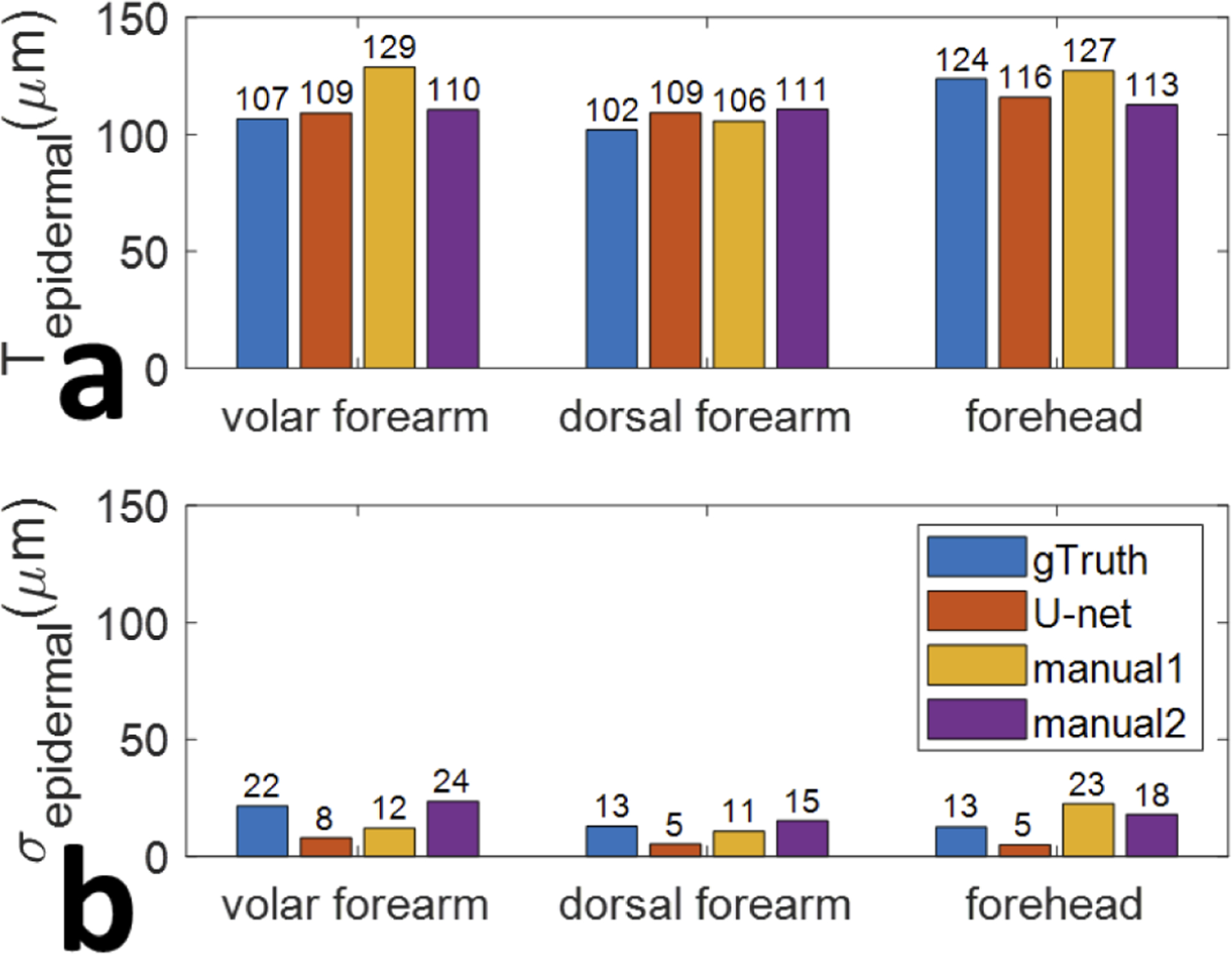
Average epidermal thickness (a) and the corresponding standard deviation of the assessment (b), gathered from five unique subjects at skin sites 1, 2, and 3, evaluated using different methods: ground truth, U-net segmentation, first manual measurement, and second manual measurement.

To quantitatively evaluate the accuracy of epidermal thickness assessment, we concatenated values of epidermal thickness obtained using ground truth annotation into a 1D vector T_gt. T_gt has 15 elements corresponding to epidermal thicknesses at 3 skin sites for 5 subjects. Similarly, we concatenated values of epidermal thickness obtained through U-Net segmentation and manual measurement into 1D vectors T_U−net, T_manual1, and T_manual2.We calculated the correlation coefficients between epidermal thickness measurements obtained with different methods (T_gt, T_U−net, T_manual1, and T_manual2) and summarize the results in Table 3. A large correlation coefficient indicates that two methods generate similar assessment of epidermal thickness, and vice versa. Table 3 shows that the consistency between U-Net analysis and ground truth annotation in epidermal thickness assessment is the highest. The correlation coefficient between T_gt and T_U−net is 0.77, while the correlation coefficient between T_gt and T_manual1 is 0.65, and the correlation coefficient between T_gt and T_manual2 is 0.52. Moreover, the disparity between measurement carried out by different individuals is large (XCC(T_manual1, T_manual2) = 0.31), suggesting large interobserver variation. The manual measurements are difficult to perform reliably. First, the measurement was performed using the cursor in ImageJ at discrete lateral locations, and was affected by the noise. Second, the dermal-epidermal junction was determined subjectively.

Table 3.

Correlation coefficients between epidermal thicknesses evaluated based on ground truth, U-net segmentation, first manual measurement, and second manual measurement.

	Ground truth	U-net	Manual1	Manual2
Ground truth	1	0.77	0.65	0.52
U-net	0.77	1	0.33	0.4
Manual1	0.65	0.33	1	0.31
Manual2	0.52	0.4	0.31	1

We further validated the effectiveness of U-Net to delineate skin images obtained from body sites other than ones in the training data set. An independent set of measurements was conducted on a healthy subject. Three manual scans each with a dimension of 512 (axial) × 1024 (lateral) were obtained from the neck and the upper arm. The neck was selected due to the high occurrence of NMSC in the region of the head and neck, and the upper arm is known to have a thinner epidermis compared to the neck [25]. Using previously described methods, we segmented the images using U-net, quantified the thickness of epidermis for each Ascan, averaged epidermal thickness within an image and across images obtained from the upper arm and neck, and show the results in Fig. 9. Our results confirm that the epidermis is thicker in the neck region compared to the upper arm.

Fig. 9.

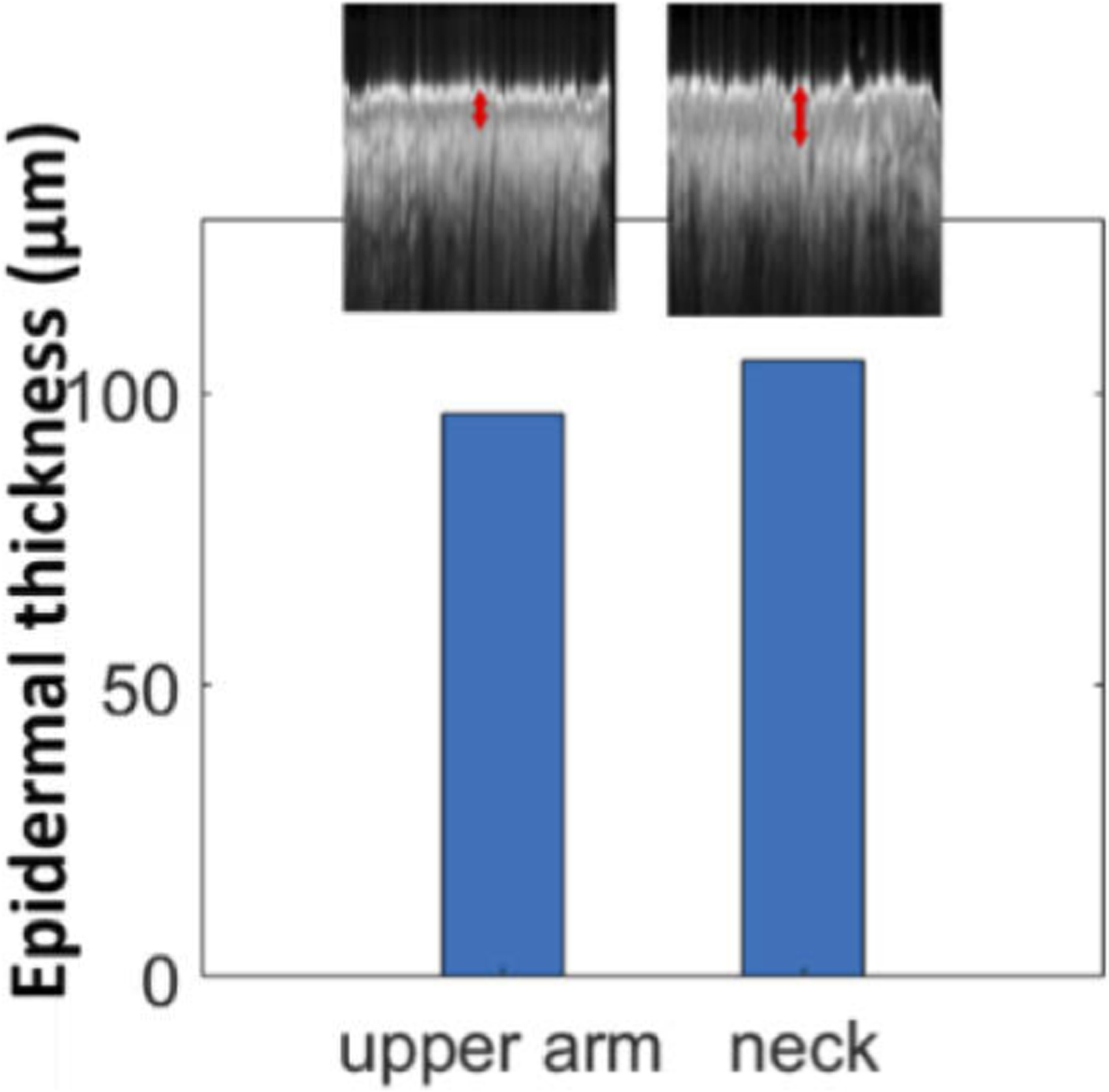
Epidermal thickness evaluated through U-Net delineation for OCT images obtained from the upper arm and neck.

3.4. Quantitative assessment of epidermal thickness of skin lesions based on U-Net delineation

Our results obtained from healthy subjects (Table 2) show that U-Net segmentation enables quantitative assessment of epidermal thickness. In addition, when correlated with the ground truth, U-Net segmentation provided higher accuracy in epidermal thickness assessment compared to manual measurement (Table 3). The thickness of epidermis varies as skin type, age and body location. Moreover, epidermal thickness is closely related to the pathological condition of the skin. For example, the development of skin tumor often results in disruption of dermal-epidermal junction (DEJ) and an altered epidermal thickness. Hence epidermal thickness of a skin lesion extracted through U-Net segmentation can be used to guide clinical diagnosis and surgical excision. Particularly, to assist Mohs micrographic surgery with AI-functionalized sfOCT imaging, it is important to demonstrate the capability of OCT imaging in differentiating skin under various conditions: normal, scar, and tumor. This is because in the majority of cases, the tumor to be removed by MMS has previously been sampled via biopsy to histopathologically confirm its nature. Therefore, the surgical site may be a combination of residual tumor, scar tissue, and surrounding normal skin. To demonstrate how the results of U-Net segmentation is related to tissue status, we performed manual scans across skin lesions along trajectories illustrated in Fig. 10. The margin of the lesion (brown area in Fig. 10) was marked by a metallic pen (blue circle in Fig. 10). Four scans across the margin were acquired. Ascans were sampled with a large lateral interval (~50μm) to achieve a large lateral field of view. Each 2D image was obtained through manual scanning. Manual scan started from the center of the lesion, moved beyond the margin labeled by the metallic pen, and ended at the normal skin. Hence, the OCT images obtained show abnormal skin (scar or tumor) on the left and normal skin on the right.

Fig. 10.

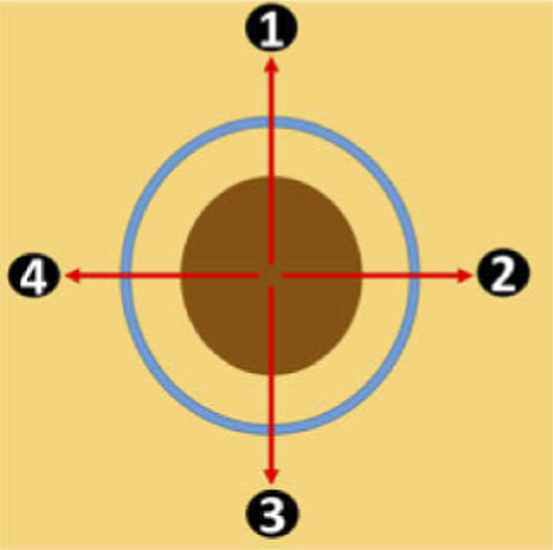
Manual scanning of a skin lesion, with brown area indicating abnormal skin (scar or tumor), yellow area indicating normal skin, and the blue circle indicating the margin marked by a metallic pen.

Two skin lesions were investigated. One was a scar induced by laser irradiation. The other was a skin tumor. The scar we imaged was located at the forearm of the subject. The scar was formed by irradiating the skin with CO₂ fractional laser (5 mJ, density 40% laser pulses) seven days prior to the imaging experiments. The age of the scars evaluated corresponds to the proliferative stage of wound healing [26] – correlating to the timeline when a patient would typically return for MMS of a tumor that had recently been biopsied. Figure 11(a) shows a picture of the scar. Results obtained from manual scans along 12 o’clock, 3 o’clock, 6 o’clock, and 9 o’clock directions (trajectories 1, 2, 3, and 4 in Fig. 10) are shown in the 1st, 2nd, 3rd and 4th columns in Fig. 11. Scale bars in Fig. 11 represent 500μm. As shown in Fig. 11(b), the region with high surface reflectivity (red arrow) corresponds to the mark made by the metallic pen. The right side of the image shows normal skin. In comparison, the scar tissue on the left side of the image shows a thin and bright surface layer, followed by a signal void layer with significantly reduced OCT magnitude and then a layer with increased signal magnitude. Figure 11(c) shows the results of U-Net segmentation for Fig. 11(b). For normal skin, the layer identified as epidermis by U-Net has a slowly varying thickness along the lateral dimension. As to the scar tissue, the layer identified as epidermis by U-Net has significantly different thickness along the lateral dimension. The quantification of epidermal thickness is further illustrated in Fig. 11(d). The thickness of the epidermis fluctuates drastically within the lesion and diminishes to zero at some locations, suggesting an altered skin structure associated with scarring. Results obtained from other scanning trajectories (Fig. 11(e)–(g) for 3 o’clock scanning, Fig. 11(h)–(j) for 6 o’clock scanning, Fig. 11(k)–(m) for 9 o’clock scanning) show similar contrast between normal skin and the scar.

Fig. 11.

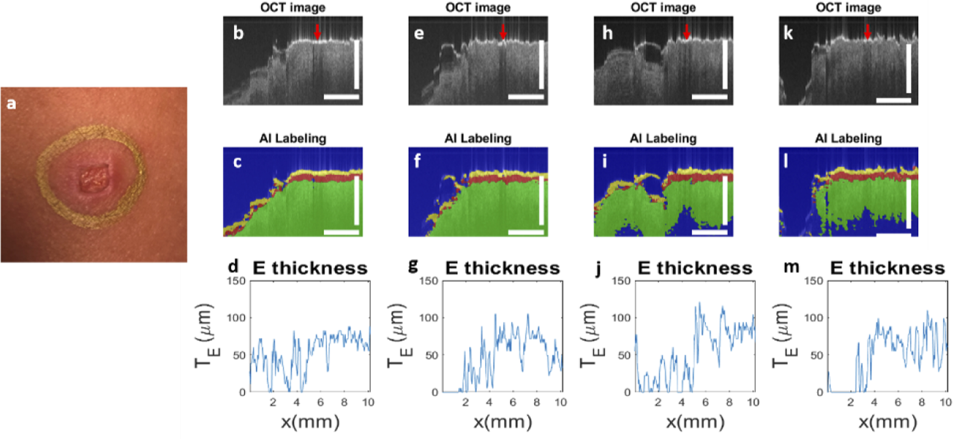
(a) photo of the scar induced by laser irradiation; results obtained by scanning along trajectory 1 (12 o’clock direction): (b) OCT image, (c) U-Net segmentation and (d) epidermal thickness quantified; results for trajectory 2 (3 o’clock direction): (e) OCT image, (f) U-Net segmentation and (g) epidermal thickness quantified; results for trajectory 3 (6 o’clock direction): (h) OCT image, (i) U-Net segmentation and (j) epidermal thickness quantified; results for trajectory 4 (9 o’clock direction): (k) OCT image, (l) U-Net segmentation and (m) epidermal thickness quantified. Scale bars represent 500μm.

We also evaluated OCT imaging and U-Net segmentation on a skin tumor. We performed manually scanned OCT imaging on patients who were scheduled to receive MMS for a biopsy-proven BCC or SCC tumor. Results shown here were obtained from a patient with SCC at his forehead. Prior to imaging, the Mohs surgeon (B.R.) used a metallic marking pen to draw the surgical margin along which the first stage would be excised. Figure 12(a) shows the picture of the skin tumor. Similar to Fig. 11, results obtained from manual scans along different trajectories are shown in the 1st, 2nd, 3rd and 4th columns in Fig. 12. Scale bars in Fig. 12 represent 500μm. Figure 12(b) shows the OCT image obtained through manual scanning along the 12 o’clock trajectory, where the red arrow indicates the mark of the metallic pen. The right side of the image shows normal skin. In comparison, the tumor on the left side of the image shows a thin and bright surface layer. Underneath the layer, the OCT signal decays at a faster rate, compared to the decay in normal skin. This is consistent with the clinical photo in Fig. 12(a) that shows a tumor with a translucent appearance because of reduced scattering. Figure 12(c) shows the result of U-Net segmentation. For normal skin, ordinary skin architecture is detected (the right side of the image). For the skin tumor, U-Net classifies most pixels underneath the surface layer as “background” pixels, because of the low signal magnitude and lack of structural features. As a result, the thickness of epidermis determined through U-Net segmentation (Fig. 12(d)) is small and varies significantly along the lateral dimension. Results obtained from other scanning trajectories (Fig. 12(e)–(g), Fig. 12(h)–(j), Fig. 12(k)–(m)) show similar contrast between normal skin and the tumor.

Fig. 12.

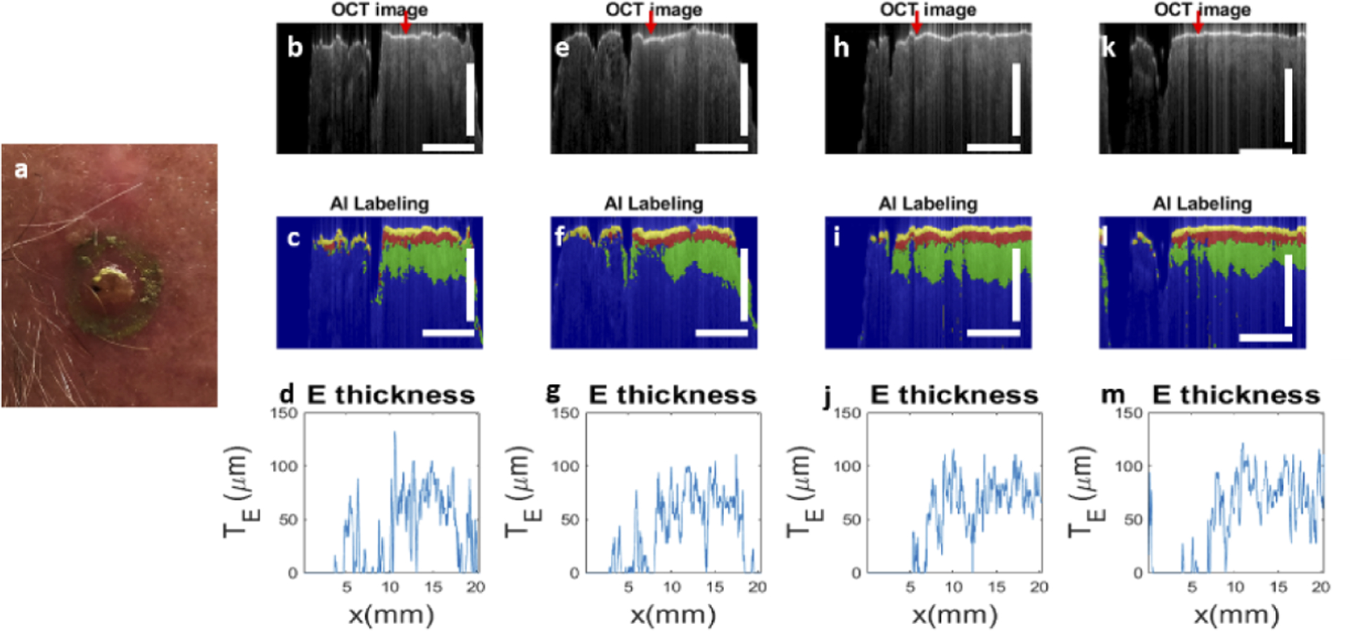
(a) Photo of the tumor; results for trajectory 1 (12 o’clock direction): (b) OCT image, (c) U-Net segmentation and (d) epidermal thickness quantified; results for trajectory 2 (3 o’clock direction): (e) OCT image, (f) U-Net segmentation and (g) epidermal thickness quantified; results for trajectory 3 (6 o’clock direction): (h) OCT image, (i) U-Net segmentation and (j) epidermal thickness quantified; results for trajectory 4 (9 o’clock direction): (k) OCT image, (l) U-Net segmentation and (m) epidermal thickness quantified. Scale bars represent 500μm.

Results in Fig. 11 and 12 demonstrate the effectiveness of OCT in differentiating skin lesions and normal skin. U-Net segmentation highlights OCT characteristics for different skin tissues and facilitates the interpretation of OCT data through visualization. Moreover, through U-Net segmentation, one can reduce massive OCT data into more concise representations that can be correlated with skin pathology for clinical applications.

4. Conclusion and discussion

In summary, we demonstrated the capability of a manually scanned OCT imager, assisted with a U-Net, for quantitative characterization of skin tissue. We acquired training data from healthy subjects, trained the U-Net, and used the U-Net to delineate normal skin and skin lesions. Our results suggest that a single fiber OCT instrument functionalized with an AI algorithm has the potential to become a cost-effective tool in clinical dermatology, to assist diagnosis and guide surgical removal of skin lesion.

In this study, the U-net was trained with OCT images and ground truth established through manual annotation. The ground truth was inherently subjective and with limited accuracy. However, for in vivo OCT imaging, it is impossible to establish a more rigorous ground truth, such as through correlation with histology. Hence, the U-Net is trained to generate results similar to manual annotation and resemble human perception. Once trained, the U-Net performs automatic image segmentation that allows quantitative extraction of clinically relevant information, such as the thickness of epidermis. In terms of speed and consistency, U-Net delineation is more advantageous compared to visual inspection and manual segmentation, as suggested by Table 3.

Our results show epidermal thickness ranging from 70μm to 150μm (Table 2). Overall, our measurements are similar to values determined by Maiti et al using OCT [25]. However, an earlier study by Mogensen et al reported slightly thinner epidermis (~80μm for most body sites imaged [23]). The disparity may derive from differences in subjects’ age, gender, skin type, and sun exposure history. Additionally, varying methods used to quantify epidermal thickness in different studies may also explain the inconsistency between the two studies. The thickness of epidermis was delineated manually on the computer screen by Mogensen et al [23], while delineated through automatic DEJ detection by Maiti et al [27]). Similarly, discrepancies exist in results obtained using other methods, such as reflectance confocal microscopy and line-field confocal OCT [24 and 28].

We implemented a U-Net with a typical architecture. The number of encoder and decoder stages, the number of filters, and the dimension of the image patch used for training were chosen empirically to optimize the outcome of segmentation. The optimization of U-Net architecture is beyond the scope of this study. One limitation of this study is the small size of data set used to train the deep learning algorithm. Nevertheless, U-Net is known to be able to produce robust segmentation when trained with a small number of examples. In addition, normal skin generally has a similar morphology, with a thin bright layer of stratum corneum, epidermis, and a less scattering dermis with signal amplitude decreasing with depth. Hence, the U-net trained with a small number of images can be used to segment these layers and quantify epidermal thickness. This is an important first step to recognizing normal skin from abnormal skin.

We used normal skin images to train the U-Net, and subsequently used the U-Net to analyze images of skin lesions. The data set used to train the U-net does not include images of scar and tumor. Therefore, the deep learning algorithm was not trained to recognize skin lesions. Instead, for signal obtained from skin lesions, the U-Net segmentation generated a high-level representation of skin architecture that was significantly different from that of normal skin. This can be used to assist with diagnosis and tumor excision. On the other hand, it is possible to train the deep learning algorithm, using images and corresponding labels from both tumor and normal skin to perform binary classification (normal versus abnormal). However, our data suggested that OCT images obtained from tumor show distinctively different features, depending on tumor type (BCC or SCC), history of biopsy, and other patient-related factors. Our future work will incorporate images obtained from a large number of patients undergoing MMS for NMSC, in order to establish a robust network. Although it is challenging to establish a large annotated image bank of diseased tissue for network training, we believe it is feasible to differentiate normal skin and skin lesion using a network trained by images of normal skin. In the future, we will use such a U-Net to segment skin images. Using features extracted from U-Net segmentation (mean and variation for the thickness of different skin layers, attenuation coefficients, etc), we will be able to establish a machine learning classifier that performs one-class detection and identifies outliers (lesions).

Data availability.

Data underlying the results presented in this paper are not publicly available at this time but may be obtained from the authors upon reasonable request.

References

- 1.Huang D, Swanson EA, Lin CP, Schuman JS, Stinson WG, Chang W, Hee MR, Flotte T, Gregory K, and Puliafito CA, “Optical coherence tomography,” Science 254(5035), 1178–1181 (1991). [DOI] [PMC free article] [PubMed] [Google Scholar]
- 2.Swanson EA, Izatt JA, Hee MR, Huang D, Lin C, Schuman J, Puliafito C, and Fujimoto JG, “In vivo retinal imaging by optical coherence tomography,” Opt. Lett 18(21), 1864–1866 (1993). [DOI] [PubMed] [Google Scholar]
- 3.Drexler W and Fujimoto JG, “State-of-the-art retinal optical coherence tomography,” Prog. Retinal Eye Res 27(1), 45–88 (2008). [DOI] [PubMed] [Google Scholar]
- 4.Welzel J, “Optical coherence tomography in dermatology: a review,” Skin Res. Technol.: Rev. article 7(1), 1–9 (2001). [DOI] [PubMed] [Google Scholar]
- 5.Welzel J, Lankenau E, Birngruber R, and Engelhardt R, “Optical coherence tomography of the human skin,” J. Am. Acad. Dermatol 37(6), 958–963 (1997). [DOI] [PubMed] [Google Scholar]
- 6.Mogensen M, Joergensen TM, Nürnberg BM, Morsy HA, Thomsen JB, Thrane L, and Jemec GB, “Assessment of optical coherence tomography imaging in the diagnosis of non-melanoma skin cancer and benign lesions versus normal skin: observer-blinded evaluation by dermatologists and pathologists,” Dermatol. Surg 35(6), 965–972 (2009). [DOI] [PubMed] [Google Scholar]
- 7.Coleman AJ, Richardson TJ, Orchard G, Uddin A, Choi MJ, and Lacy KE, “Histological correlates of optical coherence tomography in non-melanoma skin cancer,” Skin Res. Technol 19(1), e10–e19 (2013). [DOI] [PubMed] [Google Scholar]
- 8.Alawi SA, Kuck M, Wahrlich C, Batz S, McKenzie G, Fluhr JW, Lademann J, and Ulrich M, “Optical coherence tomography for presurgical margin assessment of non-melanoma skin cancer–a practical approach,” Exp. Dermatol 22(8), 547–551 (2013). [DOI] [PubMed] [Google Scholar]
- 9.Taghavikhalilbad A, Adabi S, Clayton A, Soltanizadeh H, Mehregan D, and Avanaki MR, “Semi-automated localization of dermal epidermal junction in optical coherence tomography images of skin,” Appl. Opt 56(11), 3116–3121 (2017). [DOI] [PubMed] [Google Scholar]
- 10.Weissman J, Hancewicz T, and Kaplan P, “Optical coherence tomography of skin for measurement of epidermal thickness by shapelet-based image analysis,” Opt. Express 12(23), 5760–5769 (2004). [DOI] [PubMed] [Google Scholar]
- 11.Bashkansky M and Reintjes J, “Statistics and reduction of speckle in optical coherence tomography,” Opt. Lett 25(8), 545–547 (2000). [DOI] [PubMed] [Google Scholar]
- 12.Sharma U, Fried NM, and Kang JU, “All-fiber common-path optical coherence tomography: sensitivity optimization and system analysis,” IEEE J. Sel. Top. Quantum Electron 11(4), 799–805 (2005). [Google Scholar]
- 13.Kang JU, Han J-H, Liu X, Zhang K, Song CG, and Gehlbach P, “Endoscopic functional Fourier domain common-path optical coherence tomography for microsurgery,” IEEE J. Sel. Top. Quantum Electron 16(4), 781–792 (2010). [DOI] [PMC free article] [PubMed] [Google Scholar]
- 14.Liu X, Huang Y, and Kang JU, “Distortion-free freehand-scanning OCT implemented with real-time scanning speed variance correction,” Opt. Express 20(15), 16567–16583 (2012). [Google Scholar]
- 15.Wang Y, Wang Y, Akansu A, Belfield KD, Hubbi B, and Liu X, “Robust motion tracking based on adaptive speckle decorrelation analysis of OCT signal,” Biomed. Opt. Express 6(11), 4302–4316 (2015). [DOI] [PMC free article] [PubMed] [Google Scholar]
- 16.Ronneberger O, Fischer P, and Brox T, “U-net: Convolutional networks for biomedical image segmentation,” in International Conference on Medical image computing and computer-assisted intervention, (Springer, 2015), 234–241. [Google Scholar]
- 17.Roy AG, Conjeti S, Karri SPK, Sheet D, Katouzian A, Wachinger C, and Navab N, “ReLayNet: retinal layer and fluid segmentation of macular optical coherence tomography using fully convolutional networks,” Biomed. Opt. Express 8(8), 3627–3642 (2017). [DOI] [PMC free article] [PubMed] [Google Scholar]
- 18.Venhuizen FG, van Ginneken B, Liefers B, van Grinsven MJ, Fauser S, Hoyng C, Theelen T, and Sánchez CI, “Robust total retina thickness segmentation in optical coherence tomography images using convolutional neural networks,” Biomed. Opt. Express 8(7), 3292–3316 (2017). [DOI] [PMC free article] [PubMed] [Google Scholar]
- 19.Del Amor R, Morales S, Colomer A, Mogensen M, Jensen M, Israelsen NM, Bang O, and Naranjo V, “Automatic segmentation of epidermis and hair follicles in optical coherence tomography images of normal skin by convolutional neural networks,” Front. Med 7, 220 (2020). [DOI] [PMC free article] [PubMed] [Google Scholar]
- 20.Kepp T, Droigk C, Casper M, Evers M, Hüttmann G, Salma N, Manstein D, Heinrich MP, and Handels H, “Segmentation of mouse skin layers in optical coherence tomography image data using deep convolutional neural networks,” Biomed. Opt. Express 10(7), 3484–3496 (2019). [DOI] [PMC free article] [PubMed] [Google Scholar]
- 21.De Carvalho N, Schuh S, Kindermann N, Kästle R, Holmes J, and Welzel J, “Optical coherence tomography for margin definition of basal cell carcinoma before micrographic surgery—recommendations regarding the marking and scanning technique,” Skin Res. Technol 24(1), 145–151 (2018). [DOI] [PubMed] [Google Scholar]
- 22.Zhou X, In D, Chen X, Bruhn HM, Liu X, and Yang Y, “Spectral 3D reconstruction of impressionist oil paintings based on macroscopic OCT imaging,” Appl. Opt 59(15), 4733–4738 (2020). [DOI] [PubMed] [Google Scholar]
- 23.Mogensen M, Morsy HA, Thrane L, and Jemec GB, “Morphology and epidermal thickness of normal skin imaged by optical coherence tomography,” Dermatology 217(1), 14–20 (2008). [DOI] [PubMed] [Google Scholar]
- 24.Monnier J, Tognetti L, Miyamoto M, Suppa M, Cinotti E, Fontaine M, Perez J, Orte Cano C, Yélamos O, and Puig S, “In vivo characterization of healthy human skin with a novel, non-invasive imaging technique: line-field confocal optical coherence tomography,” J. Eur. Acad. Dermatol. Venereol 34(12), 2914–2921 (2020). [DOI] [PubMed] [Google Scholar]
- 25.Maiti R, Duan M, Danby SG, Lewis R, Matcher SJ, and Carré MJ, “Morphological parametric mapping of 21 skin sites throughout the body using optical coherence tomography,” J. Mech. Behav. Biomed. Mater 102, 103501 (2020). [DOI] [PubMed] [Google Scholar]
- 26.Gurtner GC, Werner S, Barrandon Y, and Longaker MT, “Wound repair and regeneration,” Nature 453(7193), 314–321 (2008). [DOI] [PubMed] [Google Scholar]
- 27.Maiti R, Gerhardt L-C, Lee ZS, Byers RA, Woods D, Sanz-Herrera JA, Franklin SE, Lewis R, Matcher SJ, and Carré MJ, “In vivo measurement of skin surface strain and sub-surface layer deformation induced by natural tissue stretching,” J. Mech. Behav. Biomed. Mater 62, 556–569 (2016). [DOI] [PubMed] [Google Scholar]
- 28.Robertson K and Rees JL, “Variation in epidermal morphology in human skin at different body sites as measured by reflectance confocal microscopy,” Acta Derm. Venerol 90(4), 368–373 (2010). [DOI] [PubMed] [Google Scholar]
Associated Data
This section collects any data citations, data availability statements, or supplementary materials included in this article.
Data Availability Statement