First Novel Workflow for Semiquantification of Emerging Contaminants in Environmental Samples Analyzed by Gas Chromatography–Atmospheric Pressure Chemical Ionization–Quadrupole Time of Flight–Mass Spectrometry

Abstract

The ionization efficiency of emerging contaminants was modeled for the first time in gas chromatography-high-resolution mass spectrometry (GC-HRMS) which is coupled to an atmospheric pressure chemical ionization source (APCI). The recent chemical space has been expanded in environmental samples such as soil, indoor dust, and sediments thanks to recent use of high-resolution mass spectrometric techniques; however, many of these chemicals have remained unquantified. Chemical exposure in dust can pose potential risk to human health, and semiquantitative analysis is potentially of need to semiquantify these newly identified substances and assist with their risk assessment and environmental fate. In this study, a rigorously tested semiquantification workflow was proposed based on GC-APCI-HRMS ionization efficiency measurements of 78 emerging contaminants. The mechanism of ionization of compounds in the APCI source was discussed via a simple connectivity index and topological structure. The quantitative structure–property relationship (QSPR)-based model was also built to predict the APCI ionization efficiencies of unknowns and later use it for their quantification analyses. The proposed semiquantification method could be transferred into the household indoor dust sample matrix, and it could include the effect of recovery and matrix in the predictions of actual concentrations of analytes. A suspect compound, which falls inside the application domain of the tool, can be semiquantified by an online web application, free of access at http://trams.chem.uoa.gr/semiquantification/.

Introduction

Dust samples from indoor environments are a type of environmental sample that can play a major role in understanding human exposure to emerging contaminants or other chemicals of concern.¹ The numbers of chemicals found in dust samples have been growing intensively owing to the recent advances in high-resolution analytical techniques such mass spectrometry. More than 2300 chemicals were tentatively identified and reported in household indoor dust samples.² The collaborative trial in the analysis of dust samples done by the NORMAN network has found that liquid chromatography-high-resolution mass spectrometry coupled to electrospray ionization source (LC-ESI-MS) could enable tentative identification of nearly 1000 compounds.² Therefore, it would be complementary to the gas chromatography mass spectrometry coupled to electron impact (GC-EI-MS) which is designed for nonpolar areas of chemical space. The identification of nonpolar and volatile substances is not as easy as other soft ionization sources due to the complex MS1 and MS/MS fragmentation patterns of precursor ions. The GC-HRMS technique with soft ionization methods such as atmospheric pressure chemical ionization (APCI) could also provide valuable information such as identification of less LC amendable compounds and also compounds that are not ionizable in ESI.^3,4 For instance, it has been discovered that the full characterization of chlorinated paraffin mixtures can be achieved easily via the GC-APCI-MS technique in contrast to other techniques.²

Unlike the ESI source, the ionization process is quite different in the APCI source. The high voltage in APCI is not applied to the probe tip, and the nebulization and ionization occur independently. The ionization process in APCI occurs in the heated source and corona discharge needle with high voltage where the suspected compounds are ionizing. Around the corona needle, the chemical ionization reagent gas plasma (usually using pure N₂ as nebulizer gas) is being formed, and while molecules pass through this region, the ionization occurs either by charge transfer or proton transfer to produce [M+H/–H]^± or [M-H₂O+H/–H]^± ions.⁵ Therefore, the main advantage of APCI in contrast to the EI source is ease of derivation of molecular ions and the adduct forms similar to ESI. Generally, APCI is used for less-polar compounds that do not ionize efficiently under ESI. Nevertheless, some types of compounds are also too nonpolar for APCI. Therefore, GC-APCI-MS is considered complementary to ESI and the EI ionization source in terms of the chemical space that they can cover.^2,6,7

GC-APCI-HRMS has recently attracted attention and has proven valuable in not-target screening (NTS) studies of emerging contaminants due to the fact that the computational resources developed for ESI can be used often for interpretation of APCI MS/MS data.^5,7 Another advantage is that the GC retention index library can be used to assist identifications during screening of APCI chromatographic data.⁸ Finally, it enables simultaneous detection and quantification of emerging contaminants in environmental samples and provides efficient ionization efficiency.^5,7 As the use of GC-APCI-HRMS gains popularity among scientific communities,^6,7,9−11 there is a demand for developments in in silico structural annotation tools, ionization efficiency scale, and analytical method developments as well as semiquantitative or quantitative analysis. Development of a strategy toward an ionization efficiency scale of GC-APCI amendable compounds as well as their semiquantification in real environmental samples would be a breakthrough. Since the majority of newly identified compounds through nontarget analysis would not have commercial reference standards, semiquantitative analysis is a key step to finalize the risk assessment of a chemical.

Many in silico-based methods have been developed to turn the MS signal into a quantitative value for a compound when there is no reference standard available.¹²⁻¹⁷ Briefly, these methods use similar chemical structures¹⁸ or chemical properties,¹⁵ close chromatographically eluting compounds,¹⁶ parent compounds (in case of degradation or transformation products),¹⁴ and ionization efficiency.^17,19,20 Among these semiquantification methods, the use of a logarithmic scale of relative ionization efficiency (logIE) outperforms the other methods in terms of accuracy and application domain. LogIE data are usually modeled via quantitative structure–property relationships (QSPRs) to extend the application of the semiquantification method to unknown compounds. However, all these methods are developed for the ESI source, and currently, there are no such resources for APCI, in particular, GC-APCI-HRMS. Two papers have been published in the literature which used several PAHs to semiquantify their nitro-PAHs and oxo-PAHs derivatives in a GC-atmospheric pressure solid analysis probe (ASAP)-HRMS.^21,22 Semiquantifying based on similar chemical structures has been found to produce larger errors than ionization efficiency-based approaches.^12,14 Moreover, this cannot be implemented easily in case of nontarget screening or analytical methods designed for emerging pollutants which include various chemical classes.¹² To the author’s knowledge, only one work exists discussing the development of the ionization scale for APCI; however, it is developed for LC-APCI-MS instruments and a limited number of compounds (not emerging contaminants).²³ Therefore, the ionization efficiency of compounds detectable in GC-APCI-HRMS needs to be investigated in order to draw a semiquantitative conclusion. The two main obstacles in logIE-based semiquantification is to decrease the matrix effect (ME) in the case of real samples and to compensate for the analyte loss (drop in slope and calibration curve quality) during sample preparation encoded in recovery (Rec%) values.²⁴ The matrix effect can be resolved either by use of a clean-up analytical procedure and simple dilution^16,25,26 or direct projection of logIE values into a sample matrix.²⁰ The benefit of projecting logIE values to a sample matrix is to derive a predicted ME value for an analyte before analysis and evaluation of its MS signal. Latest efforts to compensate for analyte loss due to sample preparation (using solid phase extraction procedure (SPE)) and incorporation of recovery data in the semiquantitative approach has been unsuccessful.¹⁶ Nevertheless, the challenges such as Rec% and ME% estimations for a newly identified compound should be addressed in order to resolve the bias caused by either the matrix of the sample or analytical method.

This study aimed to develop the first and novel semiquantification strategy to estimate the concentrations of emerging contaminants that are measured by GC-APCI-HRMS in the presence of real environmental matrices such as household indoor dust samples. The uncertainty and application domain study for an unknown compound and mechanisms of ionization of chemicals in APCI are discussed. The linear and nonlinear modeling strategies are also evaluated. The possibility and accuracy of transferring APCI logIE data into the matrix of a real sample are presented. Finally, comprehensive guidelines are provided for a reliable semiquantitative analysis via GC-APCI-HRMS.

Experimental Section

Chemicals

Hexane and acetone (grade for pesticide analysis) were purchased from Carlo Erba Reagents (Spain). Regenerated cellulose syringe filters (RC; 15 mm diameters and 0.2 μm pore size) were purchased from Phenomenex (USA). A stock solution of the available internal standard (Atrazine-d5) was prepared at 1.0 mg L^–1 in hexane (grade for pesticide analysis). Industrial chemicals standards were purchased from Merck-Sigma-Aldrich and Riedel-de Haen (Germany). Pharmaceutical standards were purchased from Merck-Sigma-Aldrich (Germany) and Alfa Aesar (USA). Pesticide reference standards were purchased from Merck-Sigma-Aldrich (Germany), Dr. Ehrenstorfer (Germany), HPC Standards GmbH (Germany), and Fluka-Honeywell (USA). Illicit drugs were donated by the Doping Control Laboratory of the Olympic Sports Center of Athens “Spiros Louis”. Polyaromatic hydrocarbon (PAHs), polybrominated diphenyl ethers (PBDEs), polychlorinated biphenyl (PCBs), and organochlorine pesticides (OCPs) reference standards were purchased from Merck-Sigma-Aldrich (Germany). Polychlorinated naphthalenes (PCNs) were purchased from Dr. Ehrenstorfer (Germany). Atrazine-d5 was purchased from LGC standards (Greece). The full list of chemicals is available in Table S1 of the Supporting Information (SI).

Instrumental Analysis

The analysis was carried out by a GC-APCI-HRMS system consisting of a CP-8400 autosampler, Bruker 450 GC (gas chromatography system), and quadrupole time of flight (QToF) mass spectrometer (Maxis Impact, Bruker Daltonics, Bremen, Germany). GC was operated in a splitless injection mode, equipped with a Restek split liner with glass frit (4 mm × 6.3 mm × 78.5 mm), and the purge valve was activated 1 min after the injection. The injection volume was 1 μL. The analytical column used was a Restek Rxi-5Sil MS of 30 m (0.25 mm i.d. × 0.25 μm film thickness), and helium was used as a carrier gas at a constant flow of 1.5 mL min^–1. The GC oven was programmed as follows: 55 °C initial hold for 3 min, increase at a rate of 15 °C min^–1 to 180 °C at 11.33 min, increase at a rate of 6.5 °C min^–1 to 280 °C at 26.72 min and hold for 5 min, increase at a rate of 10 °C min^–1 to 300 °C at 33.72 min and hold for 5 min. The temperatures of the injector, GC-MS transfer line, and source were thermostated at 280, 290, and 250 °C, respectively. The QToF-MS was interfaced with an APCI source operating in positive ionization mode. The MS acquisition modes were based on data independent acquisition (DIA) and data dependent acquisition (DDA) modes, scanning between 40 and 1000 Da (m/z range) with scan frequency of 8 Hz. The calibration of the MS was performed using perfluorotributylamine (FC43) in the beginning of the sequence and in the beginning of every injection.

Sample Collection and Preparation

The indoor dust samples were gathered from household indoor dusts of domestic areas in the region of Attica, Greece, and a pooled sample (mix of all individual ones) was then created. To extract the pooled household indoor dust sample, a simple solid–liquid extraction procedure was applied according to the protocol developed for GC-QTOF-MS analysis by Moschet et al.¹ Briefly, 200 mg of the sample was spiked with internal standards and kept in contact for 30 min to be absorbed by the matrix. Then, 3 mL of hexane:acetone (2:1, v/v) was added to the sample, and the mixture was vortexed for 1 min. Then, the mixture was sonicated for 15 min under 30 °C and subsequently centrifuged at 4000 rpm for 5 min (Rotofix 32, Hettich, Tuttlingen, Germany). The supernatant was gathered, and the procedure was repeated once more. The final combined extract was evaporated under a nitrogen stream until almost dry, reconstituted to 200 μL (hexane:acetone (50:50, v/v)), and filtered through a regenerated cellulose filter (0.2 μm) before analysis.

Quantification Approach

To develop a logIE database including 78 emerging contaminants, stock solutions of individual reference standards (100 or 1000 mg L^–1) were prepared either in hexane or methanol (LC-MS grade) and stored at −20 °C in amber glass bottles. The intermediate mixed working solution (concentration was 5 mg L^–1) was prepared from all the individual ones, and then, the mix was evaporated under gentle N₂ to adjust the final solvent composition (hexane:acetone (50:50, v/v)). Afterward, six working solutions (5.000, 10.00, 30.00, 60.00, 200.0, and 300.0 μg L^–1) were prepared by appropriate dilution of this intermediate solution. Atrazine-d5 was used as the internal standard according to the injection volume load test.^26,27 This was to evaluate the linearity deviations of calibration curves as well as to decrease the batch effect and sensitivity loss of the instrument over time. The calibration curves were built after normalizing their peak areas which were calculated by dividing the peak area of each analyte with the peak area of the atrazine-d5. The appropriate linear range of the calibration curve for each analyte was established by removing any outliers. The outliers were tagged and removed by assessing the residual plots and furthermore implementing the elliptic joint confidence region (EJCR) test.²⁸ For all the emerging contaminants used here, the normalized peak areas derived from different adducts formed such as [M + H]⁺, [M]⁺/[M]^+• as well as abundant isotopes ([M/IS] > 10%) were summed before calculation of ionization efficiency valued. For quantification purposes, a pooled household indoor dust sample, that was divided into six aliquots, was used for the standard addition at 0.00 (blank sample), 40.00, 80.00, 200.0, 400.0, and 800.0 μg L^–1 with 26 emerging contaminants as the calibrant set. The role of the calibrant set was to harmonize and transfer the APCI logIE model to the matrix of the dust samples. In addition, nine compounds were used as the blind set which were prepared at 50.00, 100.0, and 200.0 μg L^–1 and spiked in the samples. The blind set had unique compounds which do not belong either to the test or training set. The concentration of the blind set was treated as an unknown in order to be semiquantified and to evaluate the accuracy of predicted concentrations. The selection of the calibrant was done by aid of the Kennard and Stone algorithm from the TOMCAT toolbox in MATLAB and can be found in Table S1.²⁹ Internal standards were spiked in this pooled sample and blanks at 200 μg L^–1.

Quality Control

In order to detect potential contamination, an analytical (reagent) blank was used. Standard solution curves as well as pooled samples and standard addition curves were injected in a single batch. For recovery calculation, a pooled household indoor dust sample was spiked at (200.0 μg L^–1) with a mix of reference standards used as the blind set and the internal standard at 200 μg L^–1 (using atrazine-d5). The ME%, recovery (Rec%), and % RSDr (relative standard deviation in the batch calculated by spiking three replicates of the sample at 200 μg L^–1) were evaluated for the compounds quantified in the household indoor dust samples. More details about the validation of the method and the screening strategies can be found in the previous work.²⁶

Stability Test

The selected compounds as the calibrant set, using the Kennard and Stone algorithm, were prepared at 10.00, 40.00, 80.00, 200.0, and 300.0 μg L^–1 and analyzed after five months. The purpose of this experiment was to evaluate whether the APCI logIE values are reproducible or not. Since the working solution (hexane as solvent) was sensitive to temperature and could be evaporated (even in freezing conditions), the stock solution was made freshly before analysis.

Semiquantification approach

The experimental APCI logIE values were obtained from the slopes in the calibration curves of individual analytical standards divided by the slope of a reference compound. The calibration curves were made after summing the normalized peak area from all adduct forms. This was needed, as compounds like PCBs, PCNs, PAHs, and brominated compounds produce various adduct forms of [M + H]⁺, [M]⁺, [M+H+1]⁺, and [M+Isotopes]⁺, or their radical forms are as abundant as their precursor ions. Here, omethoate was used as a reference compound because it showed a single adduct form of [M]⁺ which was relatively easy to integrate. Moreover, the APCI logIE value of omethoate was close to the median of the total APCI logIE range which is a good indicator of the ionization efficiency threshold in APCI, among the list of 78 emerging contaminants. This list of 78 emerging contaminants was compiled from various chemical classes such as pesticides, insecticides, herbicides, flame retardants, fungicides, pharmaceuticals, plasticizers, industrial chemicals, PAHs, PBDEs, PCBs, OCPs, and PCNs. This way, normally distributed ranges were obtained for logIE values. Another fact that was considered during selection of the reference compound was its ability to provide an acceptable MS signal in the presence of a sample matrix in order to successfully calculate the slope values in eqs 1 and 2. Table S1 provides the list of APCI logIE values (which is the logarithmic ratio of the slope from the calibration curve of each individual analytical standard divided by the slope of calibration curve of omethoate) for 78 emerging contaminants according to eq 1. The ratio of the molecular weight was considered to remove the effect of the measurement unit and molecular weight (MW) on logIE values.³⁰ For a compound in which no reference standard was available, the predicted ionization efficiency (logIE) based on QSPR was used to semiquantify it in real samples, as denoted in eq 2. Additionally, a correction factor (CF) was included in eq 2 which includes either dilution or a preconcentration factor to correct the predicted concentration based on an experimental setup. The matrix factor or recovery can also be added in the CF value to reduce the effect of ME and sample preparation on the actual concentration.

1

2

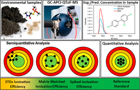
Although the logIE values are dimensionless and they do not supply any measurement unit, the unit can be comprised from the calibration curve (slopes). Here, the slopes were obtained by creating the calibration curves based on mg L^–1 unit versus normalized peak area; thus, the predicted concentration is assumed to be in mg L^–1 unit. For the quality assurance of the semiquantitative analysis, the framework proposed in our previous study was followed.²⁰ Three logIE values were created based on three calibration curves including (1) reference standards prepared in a working solution (hexane:acetone (50:50, v/v)), (2) standard addition to the matrix before analysis (matrix matched) method, and (3) standard addition to the matrix before sample extraction (spiked calibration curves). This was done to transfer the APCI logIE values derived from STDs solution to the matrix of the sample before predicting the concentration. The steps required to create ionization efficiency values in APCI are depicted in Figure 1.

Figure 1.

Derivation of experimental logIE values. (A, B) Theoretical isotopic patterns for [M+H]+ and [M]+, respectively. (C) Observed experimental isotopic pattern for BDE 28. (D) Extracted ion chromatograms (EICs) of [M+H]+ and [M]+. (E) EIC of all isotopic peaks (from B). (F) Calibration curve after summing the peak area from all isotopic peaks. (G) EIC of Omethoate ([M]+) at different concentrations. (H) Calibration curve of Omethoate as a reference compound and derivation of logIE values.

QSPR Workflow

The QSPR workflow based on the genetic algorithm (GA) coupled to multiple linear regression (GA-MLR) was used as the main modeling technique, and its details can be found in our previous works.^20,31,32 The relative importance of molecular descriptors was calculated by the “relaimpo” R package. The bootstrapped correlation coefficient function was used to describe the relationship between the most influential molecular descriptor and APCI logIE values.³³ Internal and external validation of the QSPR models were checked carefully using OECD principals (Regulation No. ENV/JM/MONO(2007)2)³⁴ and the literature.^35,36 Q²_LOO (leave one out cross validation) and Q²_LGO (leave group out cross validation) are internal accuracy measurements. Q²_Boot evaluates how dependent is a QSPR based model on the training set. Here, the data set is randomly divided 1000 times into training and test sets, and then, the cross-validated statistics are calculated. The high value of Q²_Boot shows that the QSPR model is not sensitive to the adopted training set, and other combinations of compounds in the APCI logIE database can produce a relatively acceptable model. R²_randomized and Q²_{LOOrandomized} are the maximum squared correlation coefficient and leave-one-out cross validation values, respectively, that are obtained after shuffling the molecular descriptors (X-data) 1000 times while keeping APCI logIE values (Y data) unchanged. The lower values confirm that the correlation between APCI logIE values with selected molecular descriptors is not random. Q²_Fn measures are similar to the Q²_LOO concept, but they are designed exclusively for an external test set. The modified r² value³⁷ and the concordance correlation coefficient (CCC) evaluate both accuracy and precision.^35,38 CCC evaluates the degree to which pairs of observations fall on the 45° line through the origin. The appropriate model should provide a high F_{Training/Test} value, R²_{Training/Test}, Q²_LOO, Q2_Fn, CCC_{Training/Test}, and r²_m, and low RMSE_{Training/Test}. Nevertheless, the following acceptance threshold values were applied for the remaining parameters; Q²_F1, Q²_F2, and Q²_F3 greater than 0.6; r²_m greater than 0.5; Q²_LOO/Q²_LGO/Q²_Boot greater than 0.6; R² greater than 0.7; and cutoff value of 0.85 for CCC. In addition to the QSPR acceptance criteria, the predicted concentrations of 78 reference standards at known concentrations (5.000, 10.00, 30.00, 60.00, 200.0, and 300.0 μg L^–1) were compared to the experimental data via a boxplot and distribution plot. This was done to find the averaged errors expected in low and high concentration data that were predicted based on eq 2. The Monte Carlo sampling method (MCS)³⁹ was used to find the origins of residuals and the acceptable error window in the APCI logIE model. MCS detects outliers by developing many cross-predictive models.³⁹ The results can be plotted using the absolute values of means of predictive residuals (MEAN) versus standard deviations of predictive residuals (STD). The cutoff limits for MEAN and STD were defined based on the 99% quantile of STD and MEAN calculated from the training set.³⁹ In addition to linear regression analysis, support vector regression method (SVR) was applied to model the APCI logIE data in a nonlinear manner. The three parameters in the structures of SVR models, including capacity parameter (C), Kernel function type (here radial basis function (RBF) denoted as γ), and ε-insensitive loss function, are optimized using MATLAB internal functions for SVR. More details about the SVR methodology can be found in our previous work.³¹

Software Availability

The semiquantitative analysis developed for APCI source can be performed online and freely for any suspect compound in http://trams.chem.uoa.gr/semiquantification/.

Results and Discussion

APCI logIE Modeling

Overall, 9860 molecular descriptors were calculated for each emerging contaminant. After removing the constant and intercorrelated molecular descriptors, GA selected the top seven molecular descriptors to model the experimental APCI logIE values via a simple MLR linear model. Equation 3 describes the GA-MLR model which can be used to predict APCI logIE values.

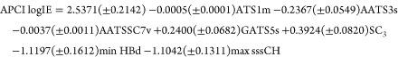3

N_train = 62, R²_train = 0.870, RMSE_train = 0.206, R²_adj = 0.852, F_train = 51.05, Q²_LOO = 0.827, Q²_LGO = 0.821, Q²_BOOT = 0.807, N_test = 16, R²_test = 0.879, RMSE_test = 0.221, rm²_test = 0.843, CCC_test = 0.934, CCC_{cross-validation} = 0.910, CCC_train = 0.930, Q²_F1 = 0.866, Q²_F2 = 0.863, Q²_F3 = 0.849, max R²_randomized = 0.114, and max Q²_{LOO randomized} = −0.183.

ATS1m (with relative importance (RI) of 52.13%) is the Moreau–Broto autocorrelation of a topological structure, lag 1/weighted by atomic masses.⁴⁰ Lag k = 1 indicates the distance between atoms pair (number of bonds between the respective atoms) in which the molecular property (here atomic mass) is calculated, and here, the interaction between neighboring atoms (lag 1) in the chemical structure is considered. It should be noted that atomic properties (indicated as w) are often centered by subtracting the average property value in the molecule to obtain proper autocorrelation values. In APCI logIE modeling, the centering function seems not to be vital. Since this molecular descriptor has accumulated more than 50% of variable importance in eq 3. The calculation of this molecular descriptor is exemplified for “cotinine” in Figure 2. In terms of MOA (mechanism of action), the lower “ATS1m” gets, the higher the ionization efficiency becomes. As depicted in Figure S1 and bootstrapped correlation analysis, a generic and simple threshold below ATS1m = 6000 can be assigned for this molecular descriptor in order to evaluate whether a compound can be potentially, highly, and sufficiently ionizable (APCI logIE > 0) in the GC-APCI-HRMS platform or not. This is a generic threshold, and future investigations by use of molecular dynamic simulation are needed. MD calculations have been developed previously to understand MOA in ESI;^41,42 however, to the best of our knowledge, there are no studies available in the literature for MD studies of GC-APCI-HRMS. Such MD calculations may evaluate possible correlations between the heat of formation of compounds (analyte and reagent ions⁴³ at atmospheric pressure) and APCI logIE values experimentally measured in this study. Two other molecular descriptors (AATS3s and AATSC7v) also belong to the Moreau–Broto autocorrelation of a topological structure. AATS3s (with RI of 4.48%) is the averaged centered type of ATS, and the atomic prosperity in this case is the I state (intrinsic state) at a topological distance of 3. AATSC7v is also an average centered ATS, and it is weighted by a van der Waals volume (with RI of 2.38%) at a topological distance of 7. GATS5s (with RI of 7.48%) is Geary autocorrelation of lag 5 weighted by the I state. Intrinsic values for various chemical moieties can be found elsewhere in the literature.^44,45 As shown, these molecular descriptors describe how the atomic property is distributed along the topological structure and represent the nearest-neighbor effect.⁴⁰ Overall, they account for 66.47% of variable importance.

Figure 2.

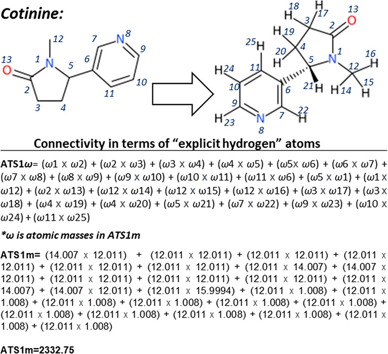
Calculation of ATS1m molecular descriptors exemplified for cotinine.

SC₃ (with RI of 12.19%) is a simple molecular connectivity Chi cluster for the third order that is based on graph isomorphism.⁴⁰ To calculate connectivity indices, every nonhydrogen atom is assigned a delta value that is calculated from its hybridization and the number of hydrogen atoms attached.⁴⁶ The order of a connectivity refers to the path length used in the chemical structure.

Therefore, the delta value is the count of neighboring atoms that are bonded to an atom in the hydrogen-suppressed graph which encodes the count of the sigma electrons contributed by that atom to bonded (nonhydrogen atoms). This descriptor is a cluster form of the Chi connectivity index, and it can reflect information about steric and branches in the chemical structure. Another descriptor in eq 3 is “minHBd” (with RI of 9.84%) which is an atom type electrotopological state, and it provides minimum e-states for (strong) hydrogen bond donors. The “maxsssCH” is maximum number of sssCH (with RI of 11.49%), and it belongs to atom type electrotopological state molecular descriptors. The first letter in sssCH is the sum of the electrotopolocial state value for the given atom in the molecule, and the second letter shows the type of bond between the atom to its neighbor nonhydrogen atom (“s”, “d”, “t”, and “a” stand for single, double, triple, and aromatic, respectively). Then, the element following is represented by its symbol and fixed hydrogen numbers. Here, for instance “sssCH” represents the sum of electrotopological state value for “_R^R > CH – R”.

Regarding the accuracy of the model (eq 3), all the QSPR-related parameters, discussed in the section “QSPR Workflow”, show acceptable values. It is noteworthy that no outlier was detected using a leverage-based⁴⁷ or chemical space boundaries approach.⁴⁸ However, at a 99% quantile, the MCS plot (Figure S2) shows that four compounds including delta-HCH, pentabromo-ethyl-benzene, theophylline, and dichlorvos have diverse chemical structures in contrast to the rest of the compounds in the training set. These structural diversities were beneficial to the model (to expand its chemical space), as the MEAN value remains low. The predicted APCI logIE values by GA-MLR and GA-SVR are plotted against the experimental logIE data (Figure 3).

Figure 3.

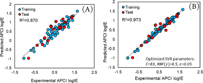
Predicted versus experimental APCI logIE values using (A) GA-MLR and (B) GA-SVR.

Internal Validation of Semiquantitative Analysis

For the internal validation of the proposed semiquantitative approach, eq 2 was used to semiquantify the compounds in Table S1. The predicted concentrations are subtracted from the actual concentrations (5.000, 10.00, 30.00, 60.00, 200.0, and 300.0 μg L^–1), and the residuals are plotted in Figure 4. In this case, the experimental logIE values (Figure 4A) as well as the predicted logIE values from GA-MLR (Figure 4B) and GA-SVR (Figure 4C) are used in eq 2. Therefore, Figure 4A depicts the error that is expected when eqs 1 and 2 are used for semiquantification purposes instead of the conventional calibration curve approach (using reference standard calibration curve, by slope and intercept). In general, when using experimental logIE values in eq 2, the mean absolute error (MAE) values for 5.000, 10.00, 30.00, 60.00, 200.0, and 300.0 μg L^–1 are 3.15, 5.44, 10.3, 12.3, 11.5, and 13.6 μg L^–1, respectively. When using predicted logIE values from GA-MLR in eq 2, the MAE values of 4.15, 7.19, 15.7, 26.6, 40.9, and 94.6 μg L^–1 are derived for 5.000, 10.00, 30.00, 60.00, 200.0, and 300.0 μg L^–1, respectively. When using the predicted logIE values from GA-SVR in eq 2, the MAE values are calculated as follows: 3.20, 5.55, 12.2, 18.5, 35.9, and 41.9 μg L^–1 for 5.000, 10.00, 30.00, 60.00, 200.0, and 300.0 μg L^–1, respectively. From Figure 4B and C, it can be concluded that the nonlinear model (GA-SVR) outperforms the linear one (GA-MLR). However, both models provide acceptable accuracy and could be used for semiquantification analysis. The advantage of the linear model is its simplicity, whereas the nonlinear model provides lower errors (especially for higher concentration data (200.0 and 300.0 μg L^–1)) than the linear model. The only disadvantages of the SVR model is that the fitting process is time consuming, and it is complex. Nevertheless, the interface for the GA-SVR calculation behind the APCI logIE model is available in the developed web-based application at http://trams.chem.uoa.gr/semiquantification/.

Figure 4.

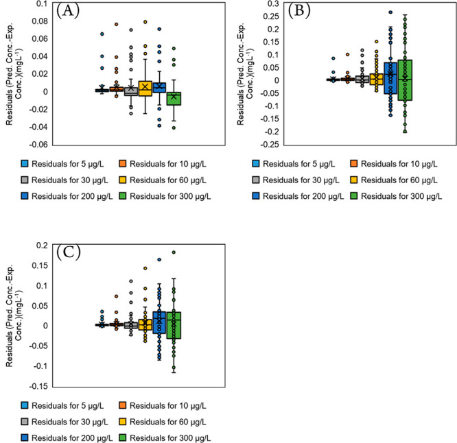
Error derived by using (A) experimental APCI logIE values and (B, C) predicted APCI logIE values for 78 compounds with known concentrations at 5.000, 10.00, 30.00, 60.00, 200.0, and 300.0 μg L^–1 via GA-MLR and GA-SVR, respectively. The y-axis simply provides the prediction error (residual = actual concentration – predicted concentration).

Stability of LogIE

The selected compounds as a calibrant set are recorded after a five-month period and depicted against the initial APCI logIE data in Figure S3. A high correlation is observed between two measurements which is a good sign for application of APCI logIE values and their analytical lifecycles. This means that the developed APCI logIE values do not require retraining for the QSPR models, and the variations between logIE data can be resolved by simple projections.

Application in Household Indoor Dust Sample

The APCI logIE values from eq 1 are projected to the matrix of indoor dust samples by simple linear regression relationships as shown in Figure 5. The 26 compounds in the calibration set show relatively better projection ability in the standard addition to the sample matrix before the extraction procedure (spiked samples, Figure 5B) than the matrix matched approach (standard addition to sample matrix before analysis). The drop in the MM calibration curve quality as well as the APCI logIE projection (Figure 5A) is due to circumstances such as formation of biphasic solutions which are required to be reevaporated and reconstituted with hexane:acetone (50:50, v/v). This process could cause analyte loss in contrast to STDs and spiked calibration curves. Nine compounds are semiquantified in indoor dust samples with known concentrations of 50.00, 100.0, and 200.0 μg L^–1. The Rec%, ME%, and RSDr% values as well as predicted concentration values for these nine compounds are available in Table 1. The Rec% values of six compounds (deltamethrin, permethrin, picoxystrobin, uniconazole, dimethylvinphos, and ethoprophos) ranged from 88.19 up to 134.81%, while the Rec% values of dimoxystrobin, flonicamid, and cypermethrin are 55.35, 57.34, and 60.27, respectively. Relatively high ME% values are also observed for these three compounds (ranging from 54.49 to 62.71), whereas the ME% values for most of the compounds are between 5.34 and 43.74. Satisfactory precision of less than 5.50% (RSDr (%)) is observed for all the compounds in Table 1. The predicted concentrations are calculated very close to the actual concentration for six out of nine compounds (deltamethrin, permethrin, cypermethrin, uniconazole, dimethylvinphos, ethoprophos) in the blind set.

Figure 5.

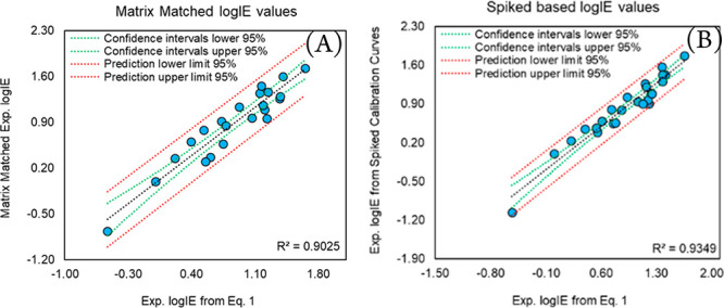
Transferability of APCI logIE values into indoor dust samples using (A) MM and (B) spiked calibration curve data.

Table 1. List of Nine Emerging Contaminants Semiquantified in Household Indoor Dust Sample.

Chemical name	Pred. logIE (GA-SVR)	Pred. concentration at 50.00 μg L–1 spiked levela	Pred. concentration at 100.0 μg L–1spiked levela	Pred. concentration at 200.0 μg L–1 spiked levela	RSDr%c	Rec%c	ME%c
Deltamethrin	0.0365	30.06 (22.47–40.22)	81.4 (60.85–108.91)	124.52 (93.07–166.59)	3.03	116.24	–11.21
Permethrin	0.5176	42.05 (35.03–50.47)	120.97 (100.77–145.21)	170.38 (141.94–204.53)	1.21	134.81	–5.34
Picoxystrobin	0.2494	145.73 (114.77–185.05)	318.57 (250.88–404.52)	537.22 (423.07–682.16)	0.37	91.78	–39.24
Cypermethrin	0.3638	12.55 (10.14–15.53)	79.79 (64.48–98.75)	140.82 (113.79–174.27)	4.56	60.27	–55.61
Uniconazole	0.5231	58.6 (48.87–70.28)	89.94 (75–107.86)	176.61 (147.27–211.8)	1.48	88.19	–41.61
Dimoxystrobin	0.1489	199.18 (153.13–259.09)	371.3 (285.45–482.97)	716.51 (550.84–932.01)	4.46	55.35	–62.71
Flonicamidb	0.1215	3.14 (2.4–4.12)	4.58 (3.5–6)	7.51 (5.73–9.83)	5.50	57.34	–54.49
Dimethylvinphos	0.294	105.86 (84.23–133.05)	186.39 (148.3–234.25)	336.04 (267.37–422.34)	1.99	128.58	–17.29
Ethoprophos	0.7665	60.96 (52.47–70.83)	165.48 (142.43–192.27)	372.68 (320.75–433.02)	2.24	97.46	–43.74

^aPredicted concentrations use the μg L^–1 unit, and the values in parentheses are lower and higher 95% CIs values calculated from the APCI logIE projection curve (Figure 5B).

^bOutside the chemical space of the model.

^cCalculated at 200.0 μg L^–1 spiked/MM level.

The real concentrations spiked in the samples (50, 100, and 200 μg L^–1) are covered or close to lower and higher CIs values for the six compounds. Since the uncertainty is defined and it accounts for the sample matrix, the upper and lower values (95% CIs) can be used and compared against the provisional no effect concentration (PNEC) in order to decide about the fates of the chemicals in the environment.²⁴ The prediction errors for picoxystrobin and dimoxystrobin are relatively high which could be due to their structural diversities in contrast to the training set. Therefore, the origin of error could relate to predicted APCI logIE data. The predicted concentration values for flonicamid have been underestimated significantly, and because they are not inside the applicability domain, this causes the predicted concentrations not to be reliable. The highly squared correlation coefficient value (R² = 0.934) is obtained when transferring the APCI logIE values into the sample matrix via a spiked calibration curve (Figure 5B). Therefore, the linear regression function can be applied to transfer the APCI logIE data from the standard solution to the spiked-based APCI logIE values. This can result in accurate estimations of the concentrations of the analytes while reducing the bias due to sample matrix or analyte loss/enhancement (sample preparation procedure). Nevertheless, creating a link between the spiked and reference standard solutions based APCI logIE data can remain challenging if the APCI logIE values show poor transferability (R² < 0.850).

Future Perspectives

The current work can contribute to nontarget screening of any environmental samples, especially dust samples, which are analyzed in GC-APCI-HRMS. The semiquantitative analysis based on ionization efficiency offers many advantages in contrast to other existing methods including better accuracy, ease of use (it decreases time and laboratory costs), ability to be applied to historical data and digital samples freezing platforms, and understanding of the matrix effect and recovery on the ionization efficiency of compounds with a wide scope of applications. Moreover, the simple MOA introduced here can help understand whether chemicals efficiently ionize in the GC-APCI-HRMS source or not, which is very useful to future chemical domain studies of analytical methods.⁴⁹ Although the uncertainty associated with ionization efficiency-based approaches is usually between 2- and 4-fold errors, which needs to be improved, it is generally acceptable in environmental science.¹² Nevertheless, future community efforts would be wise to increase the number of compounds in the APCI logIE database which can result in improved accuracies of models and expand chemical space boundaries significantly. Such efforts would expand the applications of APCI logIE for other areas than environmental science such as metabolomics and foodomics. Finally, the developed semiquantification technique may not be applicable to other similar atmospheric ionization sources such as photoionization (APPI) because the fragmentation pattern especially in terms of ion intensity can be varied.⁵⁰ Since in the development of logIE values the isotopic correction approach is applied, this would cause inaccuracy and variation in the logIE values if transferred from APCI to other similar sources. Future studies may focus on improving the transferability of logIE values across different atmospheric ionization sources using Table S1 as valuable list of chemicals developed for the APCI source.

Conclusions

Considering the modeling accuracy and MOA, it can be concluded that quantum mechanical treatment of the series of 78 emerging contaminants may not be necessary to develop structural information to correlate with APCI logIE values. The classical molecular descriptors such as autocorrelation of a topological structure and molecular connectivity index could be sufficient to derive the APCI logIE values. Even though “feeding” the models with more compounds is needed to fully understand the ionization process in the APCI source, a threshold below 6000 for ATS1m could be an indication of how well a compound would ionize in the APCI source. The lower and upper thresholds for ATS1m should be further investigated using MD calculations. The calculation of ATS1m is very simple, and it does not require any expensive computational resources for practicing chemists. The calculated APCI logIE values have been stable in a five-month intralaboratory test. This expands the lifecycle of the analytical method and the applicability of the models without requiring any retraining. The semiquantitative tool could be linearly transferred into the sample matrix using a standard addition to the sample matrix before the extraction procedure method (spiked calibration curve) (R² = 0.934). This was an important step toward inclusion of the effects of recovery and the matrix for predictions of the concentrations of analytes in real samples. The proposed work has potential applications in analyses of indoor dust samples and evaluations of their adverse effects of human health. In addition, it can be used to understand the states of ionization of the analytes of interest in GC-APCI-HRMS and if they will be detectable via GC-APCI-HRMS. We conclude that the proposed strategy gives more hope than despair in the quest for GC-APCI-HRMS-based semiquantification of emerging contaminants in real environmental samples.

Supporting Information Available

The Supporting Information is available free of charge at https://pubs.acs.org/doi/10.1021/acs.analchem.2c01432.

• Table of chemicals used in this work along with their ionization efficiency data and three figures (PDF)

Author Contributions

Conceptualization: R.A. and N.S.T. Writing, original draft and editing: R.A. and V.N. Experimental and quantitative analyses: V.N. Software: R.A., V.N., and N.A.A. Editing and formal analysis: N.A.A. and N.S.T. Supervision: R.A. and N.S.T.

Author Contributions

^§ Reza Aalizadeh and Varvara Nikolopoulou contributed equally to this work.

The authors declare no competing financial interest.

References

- Moschet C.; Anumol T.; Lew B. M.; Bennett D. H.; Young T. M. Household Dust as a Repository of Chemical Accumulation: New Insights from a Comprehensive High-Resolution Mass Spectrometric Study. Environ. Sci. Technol. 2018, 52, 2878–2887. 10.1021/acs.est.7b05767. [DOI] [PMC free article] [PubMed] [Google Scholar]
- Rostkowski P.; Haglund P.; Aalizadeh R.; Alygizakis N.; Thomaidis N.; Arandes J. B.; Nizzetto P. B.; Booij P.; Budzinski H.; Brunswick P.; Covaci A.; Gallampois C.; Grosse S.; Hindle R.; Ipolyi I.; Jobst K.; Kaserzon S. L.; Leonards P.; Lestremau F.; Letzel T.; et al. The strength in numbers: comprehensive characterization of house dust using complementary mass spectrometric techniques. Anal. Bioanal. Chem. 2019, 411, 1957–1977. 10.1007/s00216-019-01615-6. [DOI] [PMC free article] [PubMed] [Google Scholar]
- Cai S.-S.; Syage J. A. Comparison of Atmospheric Pressure Photoionization, Atmospheric Pressure Chemical Ionization, and Electrospray Ionization Mass Spectrometry for Analysis of Lipids. Anal. Chem. 2006, 78, 1191–1199. 10.1021/ac0515834. [DOI] [PubMed] [Google Scholar]
- Li X.; Dorman F. L.; Helm P. A.; Kleywegt S.; Simpson A.; Simpson M. J.; Jobst K. J. Nontargeted Screening Using Gas Chromatography–Atmospheric Pressure Ionization Mass Spectrometry: Recent Trends and Emerging Potential. Molecules 2021, 26, 6911. 10.3390/molecules26226911. [DOI] [PMC free article] [PubMed] [Google Scholar]
- Mesihää S.; Ketola R. A.; Pelander A.; Rasanen I.; Ojanperä I. Development of a GC-APCI-QTOFMS library for new psychoactive substances and comparison to a commercial ESI library. Anal. Bioanal. Chem. 2017, 409, 2007–2013. 10.1007/s00216-016-0148-y. [DOI] [PubMed] [Google Scholar]
- Pintado-Herrera M. G.; González-Mazo E.; Lara-Martín P. A. Atmospheric pressure gas chromatography–time-of-flight-mass spectrometry (APGC–ToF-MS) for the determination of regulated and emerging contaminants in aqueous samples after stir bar sorptive extraction (SBSE). Anal. Chim. Acta 2014, 851, 1–13. 10.1016/j.aca.2014.05.030. [DOI] [PubMed] [Google Scholar]
- Portolés T.; Mol J. G. J.; Sancho J. V.; Hernández F. Use of electron ionization and atmospheric pressure chemical ionization in gas chromatography coupled to time-of-flight mass spectrometry for screening and identification of organic pollutants in waters. J. Chromatogr. A 2014, 1339, 145–153. 10.1016/j.chroma.2014.03.001. [DOI] [PubMed] [Google Scholar]
- Arbulu M.; Sampedro M. C.; Unceta N.; Gómez-Caballero A.; Goicolea M. A.; Barrio R. J. A retention time locked gas chromatography–mass spectrometry method based on stir-bar sorptive extraction and thermal desorption for automated determination of synthetic musk fragrances in natural and wastewaters. J. Chromatogr. A 2011, 1218, 3048–3055. 10.1016/j.chroma.2011.03.012. [DOI] [PubMed] [Google Scholar]
- Li D.-X.; Gan L.; Bronja A.; Schmitz O. J. Gas chromatography coupled to atmospheric pressure ionization mass spectrometry (GC-API-MS): Review. Anal. Chim. Acta 2015, 891, 43–61. 10.1016/j.aca.2015.08.002. [DOI] [PubMed] [Google Scholar]
- Ojanperä I.; Mesihää S.; Rasanen I.; Pelander A.; Ketola R. A. Simultaneous identification and quantification of new psychoactive substances in blood by GC-APCI-QTOFMS coupled to nitrogen chemiluminescence detection without authentic reference standards. Anal. Bioanal. Chem. 2016, 408, 3395–3400. 10.1007/s00216-016-9461-8. [DOI] [PubMed] [Google Scholar]
- De O. Silva R.; De Menezes M. G.G.; De Castro R. C.; De A. Nobre C.; Milhome M. A.L.; Do Nascimento R. F. Efficiency of ESI and APCI ionization sources in LC-MS/MS systems for analysis of 22 pesticide residues in food matrix. Food Chem. 2019, 297, 124934. 10.1016/j.foodchem.2019.06.001. [DOI] [PubMed] [Google Scholar]
- Kruve A. Strategies for Drawing Quantitative Conclusions from Nontargeted Liquid Chromatography–High-Resolution Mass Spectrometry Analysis. Anal. Chem. 2020, 92, 4691–4699. 10.1021/acs.analchem.9b03481. [DOI] [PubMed] [Google Scholar]
- Kruve A.; Kaupmees K. Predicting ESI/MS Signal Change for Anions in Different Solvents. Anal. Chem. 2017, 89, 5079–5086. 10.1021/acs.analchem.7b00595. [DOI] [PubMed] [Google Scholar]
- Kruve A.; Kiefer K.; Hollender J. Benchmarking of the quantification approaches for the non-targeted screening of micropollutants and their transformation products in groundwater. Anal. Bioanal. Chem. 2021, 413, 1549–1559. 10.1007/s00216-020-03109-2. [DOI] [PMC free article] [PubMed] [Google Scholar]
- Kalogiouri N. P.; Aalizadeh R.; Thomaidis N. S. Investigating the organic and conventional production type of olive oil with target and suspect screening by LC-QTOF-MS, a novel semi-quantification method using chemical similarity and advanced chemometrics. Anal. Bioanal. Chem. 2017, 409, 5413–5426. 10.1007/s00216-017-0395-6. [DOI] [PubMed] [Google Scholar]
- Malm L.; Palm E.; Souihi A.; Plassmann M.; Liigand J.; Kruve A. Guide to Semi-Quantitative Non-Targeted Screening Using LC/ESI/HRMS. Molecules 2021, 26, 3524. 10.3390/molecules26123524. [DOI] [PMC free article] [PubMed] [Google Scholar]
- Panagopoulos Abrahamsson D.; Park J. S.; Singh R. R.; Sirota M.; Woodruff T. J. Applications of Machine Learning to In Silico Quantification of Chemicals without Analytical Standards. J. Chem. Inf. Model. 2020, 60, 2718–2727. 10.1021/acs.jcim.9b01096. [DOI] [PMC free article] [PubMed] [Google Scholar]
- Alygizakis N.; Galani A.; Rousis N. I.; Aalizadeh R.; Dimopoulos M.-A.; Thomaidis N. S. Change in the chemical content of untreated wastewater of Athens, Greece under COVID-19 pandemic. Sci. Total Environ. 2021, 799, 149230. 10.1016/j.scitotenv.2021.149230. [DOI] [PMC free article] [PubMed] [Google Scholar]
- Kruve A.; Kaupmees K.; Liigand J.; Leito I. Negative electrospray ionization via deprotonation: predicting the ionization efficiency. Anal. Chem. 2014, 86, 4822–4830. 10.1021/ac404066v. [DOI] [PubMed] [Google Scholar]
- Aalizadeh R.; Nikolopoulou V.; Alygizakis N.; Slobodnik J.; Thomaidis N. S. novel workflow for semi-quantification of emerging contaminants in environmental samples analyzed by LC-HRMS. Anal. Bioanal. Chem. 2022, 10.1007/s00216-022-04084-6. [DOI] [PubMed] [Google Scholar]
- Carrizo D.; Domeño C.; Nerín I.; Alfaro P.; Nerín C. Atmospheric pressure solid analysis probe coupled to quadrupole-time of flight mass spectrometry as a tool for screening and semi-quantitative approach of polycyclic aromatic hydrocarbons, nitro-polycyclic aromatic hydrocarbons and oxo-polycyclic aromatic hydrocarbons in complex matrices. Talanta 2015, 131, 175–184. 10.1016/j.talanta.2014.07.034. [DOI] [PubMed] [Google Scholar]
- Domeño C.; Canellas E.; Alfaro P.; Rodriguez-Lafuente A.; Nerin C. Atmospheric pressure gas chromatography with quadrupole time of flight mass spectrometry for simultaneous detection and quantification of polycyclic aromatic hydrocarbons and nitro-polycyclic aromatic hydrocarbons in mosses. J. Chromatogr. A 2012, 1252, 146–154. 10.1016/j.chroma.2012.06.061. [DOI] [PubMed] [Google Scholar]
- Rebane R.; Kruve A.; Liigand P.; Liigand J.; Herodes K.; Leito I. Establishing Atmospheric Pressure Chemical Ionization Efficiency Scale. Anal. Chem. 2016, 88, 3435–3439. 10.1021/acs.analchem.5b04852. [DOI] [PubMed] [Google Scholar]
- McCord J. P.; Groff L. C.; Sobus J. R. Quantitative non-targeted analysis: Bridging the gap between contaminant discovery and risk characterization. Environ. Int. 2022, 158, 107011. 10.1016/j.envint.2021.107011. [DOI] [PMC free article] [PubMed] [Google Scholar]
- Kruve A.; Leito I.; Herodes K. Combating matrix effects in LC/ESI/MS: the extrapolative dilution approach. Anal. Chim. Acta 2009, 651, 75–80. 10.1016/j.aca.2009.07.060. [DOI] [PubMed] [Google Scholar]
- Nikolopoulou V.; Aalizadeh R.; Nika M.-C.; Thomaidis N. S. TrendProbe: Time profile analysis of emerging contaminants by LC-HRMS non-target screening and deep learning convolutional neural network. J. Hazard. Mater. 2022, 428, 128194. 10.1016/j.jhazmat.2021.128194. [DOI] [PubMed] [Google Scholar]
- Yu H.; Xing S.; Nierves L.; Lange P. F.; Huan T. Fold-Change Compression: An Unexplored But Correctable Quantitative Bias Caused by Nonlinear Electrospray Ionization Responses in Untargeted Metabolomics. Anal. Chem. 2020, 92, 7011–7019. 10.1021/acs.analchem.0c00246. [DOI] [PubMed] [Google Scholar]
- González A. G.; Herrador M. A.; Asuero A. n. G. Intra-laboratory testing of method accuracy from recovery assays. Talanta 1999, 48, 729–736. 10.1016/S0039-9140(98)00271-9. [DOI] [PubMed] [Google Scholar]
- Daszykowski M.; Serneels S.; Kaczmarek K.; Van Espen P.; Croux C.; Walczak B. TOMCAT: A MATLAB toolbox for multivariate calibration techniques. Chemom. Intell. Lab. Syst. 2007, 85, 269–277. 10.1016/j.chemolab.2006.03.006. [DOI] [Google Scholar]
- Cherkasov A.; Muratov E. N.; Fourches D.; Varnek A.; Baskin I. I.; Cronin M.; Dearden J.; Gramatica P.; Martin Y. C.; Todeschini R.; Consonni V.; Kuz’min V. E.; Cramer R.; Benigni R.; Yang C.; Rathman J.; Terfloth L.; Gasteiger J.; Richard A.; Tropsha A. QSAR Modeling: Where Have You Been? Where Are You Going To?. J. Med. Chem. 2014, 57, 4977–5010. 10.1021/jm4004285. [DOI] [PMC free article] [PubMed] [Google Scholar]
- Aalizadeh R.; Thomaidis N. S.; Bletsou A. A.; Gago-Ferrero P. Quantitative Structure–Retention Relationship Models To Support Nontarget High-Resolution Mass Spectrometric Screening of Emerging Contaminants in Environmental Samples. J. Chem. Inf. Model. 2016, 56, 1384–1398. 10.1021/acs.jcim.5b00752. [DOI] [PubMed] [Google Scholar]
- Aalizadeh R.; Alygizakis N. A.; Schymanski E. L.; Krauss M.; Schulze T.; Ibáñez M.; McEachran A. D.; Chao A.; Williams A. J.; Gago-Ferrero P.; Covaci A.; Moschet C.; Young T. M.; Hollender J.; Slobodnik J.; Thomaidis N. S. Development and Application of Liquid Chromatographic Retention Time Indices in HRMS-Based Suspect and Nontarget Screening. Anal. Chem. 2021, 93, 11601–11611. 10.1021/acs.analchem.1c02348. [DOI] [PubMed] [Google Scholar]
- Pernet C. R.; Wilcox R.; Rousselet G. A. Robust correlation analyses: false positive and power validation using a new open source matlab toolbox. Front. Psychol. 2013, 3, 606–606. 10.3389/fpsyg.2012.00606. [DOI] [PMC free article] [PubMed] [Google Scholar]
- OECD Regulation, Guidance document on the validation of (quantitative) structure-activity relationships [(Q)SAR] models; OECD Series on Testing and Assessment; OECD, 2007.
- Chirico N.; Gramatica P. Real External Predictivity of QSAR Models: How To Evaluate It? Comparison of Different Validation Criteria and Proposal of Using the Concordance Correlation Coefficient. J. Chem. Inf. Model. 2011, 51, 2320–2335. 10.1021/ci200211n. [DOI] [PubMed] [Google Scholar]
- Chirico N.; Gramatica P. Real External Predictivity of QSAR Models. Part 2. New Intercomparable Thresholds for Different Validation Criteria and the Need for Scatter Plot Inspection. J. Chem. Inf. Model. 2012, 52, 2044–2058. 10.1021/ci300084j. [DOI] [PubMed] [Google Scholar]
- Roy P. P.; Roy K. On Some Aspects of Variable Selection for Partial Least Squares Regression Models. QSAR & Comb. Sci. 2008, 27, 302–313. 10.1002/qsar.200710043. [DOI] [Google Scholar]
- Lin L. A concordance correlation coefficient to evaluate reproducibility. Biometrics 1989, 45, 255–268. 10.2307/2532051. [DOI] [PubMed] [Google Scholar]
- Aalizadeh R.; Nika M. C.; Thomaidis N. S. Development and application of retention time prediction models in the suspect and non-target screening of emerging contaminants. J. Hazard. Mater. 2019, 363, 277–285. 10.1016/j.jhazmat.2018.09.047. [DOI] [PubMed] [Google Scholar]
- Todeschini R.; Consonni V.. Handbook of Molecular Descriptors; Wiley-VCH Verlag GmbH: Germany, 2000; p 1–667. [Google Scholar]
- Konermann L.; Ahadi E.; Rodriguez A. D.; Vahidi S. Unraveling the Mechanism of Electrospray Ionization. Anal. Chem. 2013, 85, 2–9. 10.1021/ac302789c. [DOI] [PubMed] [Google Scholar]
- Ahadi E.; Konermann L. Modeling the Behavior of Coarse-Grained Polymer Chains in Charged Water Droplets: Implications for the Mechanism of Electrospray Ionization. J. Phys. Chem. B 2012, 116, 104–112. 10.1021/jp209344z. [DOI] [PubMed] [Google Scholar]
- Andrade F. J.; Shelley J. T.; Wetzel W. C.; Webb M. R.; Gamez G.; Ray S. J.; Hieftje G. M. Atmospheric Pressure Chemical Ionization Source. 1. Ionization of Compounds in the Gas Phase. Anal. Chem. 2008, 80, 2646–2653. 10.1021/ac800156y. [DOI] [PubMed] [Google Scholar]
- Hall L. H.; Mohney B.; Kier L. B. The electrotopological state: structure information at the atomic level for molecular graphs. J. Chem. Inf. Comput. Sci. 1991, 31, 76–82. 10.1021/ci00001a012. [DOI] [Google Scholar]
- Qin L.-T.; Liu S.-S.; Liu H.-L. QSPR model for bioconcentration factors of nonpolar organic compounds using molecular electronegativity distance vector descriptors. Mol. Divers. 2010, 14, 67–80. 10.1007/s11030-009-9145-9. [DOI] [PubMed] [Google Scholar]
- Kier L. B.; Hall L. H.. Molecular Connectivity in Structure-Activity Analysis; Wiley, 1986. [Google Scholar]
- Gramatica P. Principles of QSAR models validation: internal and external. QSAR & Comb. Sci. 2007, 26, 694–701. 10.1002/qsar.200610151. [DOI] [Google Scholar]
- Aalizadeh R.; von der Ohe P. C.; Thomaidis N. S. Prediction of acute toxicity of emerging contaminants on the water flea Daphnia magna by Ant Colony Optimization–Support Vector Machine QSTR models. Environ. Sci.: Process. Impacts 2017, 19, 438–448. 10.1039/c6em00679e. [DOI] [PubMed] [Google Scholar]
- Lowe C. N.; Isaacs K. K.; McEachran A.; Grulke C. M.; Sobus J. R.; Ulrich E. M.; Richard A.; Chao A.; Wambaugh J.; Williams A. J. Predicting compound amenability with liquid chromatography-mass spectrometry to improve non-targeted analysis. Anal. Bioanal. Chem. 2021, 413, 7495–7508. 10.1007/s00216-021-03713-w. [DOI] [PMC free article] [PubMed] [Google Scholar]
- Di Lorenzo R. A.; Lobodin V. V.; Cochran J.; Kolic T.; Besevic S.; Sled J. G.; Reiner E. J.; Jobst K. J. Fast gas chromatography-atmospheric pressure (photo)ionization mass spectrometry of polybrominated diphenylether flame retardants. Anal. Chim. Acta 2019, 1056, 70–78. 10.1016/j.aca.2019.01.007. [DOI] [PMC free article] [PubMed] [Google Scholar]
Associated Data
This section collects any data citations, data availability statements, or supplementary materials included in this article.