

Abstract

A methodology to calculate the decay rates of normal and resonant Auger processes in atoms and molecules based on the One-Center Approximation (OCA), using atomic radial Auger integrals, is implemented within the restricted-active-space self-consistent-field (RASSCF) and the multistate restricted-active-space perturbation theory of second order (MS-RASPT2) frameworks, as part of the OpenMolcas project. To ensure an unbiased description of the correlation and relaxation effects on the initial core excited/ionized states and the final cationic states, their wave functions are optimized independently, whereas the Auger matrix elements are computed with a biorthonormalized set of molecular orbitals within the state-interaction (SI) approach. As a decay of an isolated resonance, the computation of Auger intensities involves matrix elements with one electron in the continuum. However, treating ionization and autoionization problems can be overwhelmingly complicated for nonexperts, because of many peculiarities, in comparison to bound-state electronic structure theory. One of the advantages of our approach is that by projecting the intensities on the atomic center bearing the core hole and using precalculated atomic radial two-electron integrals, the Auger decay rates can be easily obtained directly with OpenMolcas, avoiding the need to interface it with external programs to compute matrix elements with the photoelectron wave function. The implementation is tested on the Ne atom, for which numerous theoretical and experimental results are available for comparison, as well as on a set of prototype closed- and open-shell molecules, namely, CO, N2, HNCO, H2O, NO2, and C4N2H4 (pyrimidine).
1. Introduction
Of the many types of X-ray spectroscopy currently accessible, Auger electron spectroscopy1−4 is of special interest, since it encodes the electronic structure of the system into the kinetic energy of the ejected electron, mapping bound states to the continuum. The state of a molecule resulting from the photoexcitation or phototoionization of an electron from a deep core–shell is a resonance embedded in several continua, so it is usually very unstable and, thus, characterized by a rather short lifetime, from a few femtoseconds to dozens of femtoseconds.5,6 Therefore, the core–hole states decay, either by X-ray photon emission (XES), or by Auger electron emission, which is a process where the core electron vacancy is filled by one of the valence electrons and another valence electron is ejected to the continuum. In most situations, the process can be treated accurately by first-order perturbation theory as the decay of a bound state into the underlying continuum.7 The two most common types of Auger decay processes are normal Auger, exploited in normal Auger electron spectroscopy (herein indicated as AES), and resonant Auger, used in resonant Auger electron spectroscopy (RAES).1−3 Similar (nonlocal) processes are interatomic Coulomb decay (ICD)8,9 and electron transfer mediated decay (ETMD).10
The normal or nonresonant Auger process occurs when
the initial
core-ionized state (relevant for XPS) decays to a doubly ionized (double-hole)
final state. In the common case of closed-shell molecules, two series
of singlets and triplets are obtained, but the presented formalism
can easily deal with open-shell systems. The kinetic energy  of the ejected Auger electron can be obtained
by energy conservation2–i.e.,
of the ejected Auger electron can be obtained
by energy conservation2–i.e.,
and is independent of the energy of the photon used to prepare the initial ionized state. On the other hand, a resonant Auger process occurs when a core-excited state (relevant for XAS) decays to a singly ionized state, where the outgoing electron can be either the core-excited electron, resulting in a one-hole (1h) final state (participator Auger), or an inner-valence electron, resulting in a two-hole-one-particle 2h1p state (spectator Auger). The kinetic energy of the resonant Auger electron can also be determined by a simple conservation of energy,
and it clearly depends on the photon energy used to prepare the core-excited state.2
The high sensitivity of AES/RAES to electronic and nuclear dynamics encouraged experimentalists to explore it to unravel underlying electron and nuclear dynamics of photoexcited molecules.11−16 In the case of halogen-containing molecules, the photoexcited repulsive σ* states expose the competition between nuclear dynamics and resonant Auger electron emission, because of the fact that both Auger decay and direct dissociation occur on the femtosecond time scale.17−19 In a series of recent studies, it was also demonstrated that ultrafast dissociation, distinguished by means of its fingerprint in the RAES, is a practical mechanism of distributing the molecular internal energy of the L-edge photoexcited systems in small molecules like HCl17 as well as in heavier ones, such as CH2Cl2 and CHCl3.18,19 Moreover, the Auger decay around the Cl 1s threshold of HCl has been recently simulated, considering the evolution of the relaxation process, including both electron and nuclear dynamics.20 Adding to that is the fact that AES does not obey the same dipole transition rules as XAS does, so AES/RAES can be used as a powerful tool to probe dark states and couple to nuclear dynamics.11−13 However, from the computational point of view, for AES/RAES to be used effectively as a probe of (excited-state) nuclear dynamics, one should efficiently deal with one of the major complications in the computation of Auger spectra, namely the description of the electron in the continuum.
Notably, modeling processes involving electrons in the continuum remains a challenge, since the asymptotic behavior of the continuum wave function is poorly described within correlated methods based on quadratically integrable finite basis sets (L2 basis sets),21 commonly used for bound states.
Special quadrature techniques, like Stieltjes imaging22−26 or Padé approaches,27−30 have been employed with some success to overcome some of these problems. However, the absence of proper asymptotic boundary conditions in these implicit continuum methods makes the separations of individual channels ambiguous. Even though it has been demonstrated that partial decay cross sections can be calculated using a Stieltjes imaging procedure by appropriate projection techniques,9,31 this comes at the cost of employing very large basis sets, which hinders the applicability to large molecules and commonly introduces linear dependency problems. More general approaches rely on the use of a multicentric linear combination of atomic orbitals (LCAO) B-spline basis32,33 with the correct asymptotic boundary conditions of the continuum, as obtained with the B-spline static-exchange density functional theory (DFT)34−36 and time-dependent density functional theory (TD-DFT).7,37
Theoretical approaches aiming at the calculation of molecular Auger decay rates reported in the literature rely on distinct approximations of the electronic continuum wave functions. A few examples are the Stieltjes imaging method,9,31,38,39 the plane-waves and Coulomb-waves based approaches,40,41 solving the Lippmann–Schwinger equation with Gaussian basis functions,42,43 solving the one-electron radial Schrödinger equations with spherical continuum wave functions,44,45 and the one-center approximation.46−49 Where methods like those based on Stieltjes Imaging31 or on population analysis50−52 do not treat the electronic continuum wave function explicitly, the one-center approximation (OCA) uses precalculated bound-continuum integrals from atomic calculations. Moreover, the one-center approximation can be easily generalized to describe vibrational excitations53 and angular distributions.54
Electronic continuum boundary conditions often translate into a high entrance barrier for a quantum chemist used to work with bound states. Besides the inconvenience of dealing with non-L2 boundary conditions, one usually must use external codes and write interfaces to them in order to calculate one- and two-electron integrals involving simultaneously the bound and continuum orbitals. Here, a simple approach to obtain the relevant bound-continuum two-electron integrals based on the one-center approximation46−48 is directly implemented in OpenMolcas for a RASSCF/RASPT255−58 bound-state description that relies on a biorthonormalized set of molecular orbitals within the state-interaction59 approach. Our implementation lowers the barrier for a nonexpert, since it replaces the necessity to use different programs, with a very efficient protocol utilizing precalculated bound-continuum Auger integrals. Moreover, as more and more time-resolved experiments are performed at the femtosecond time scale,6,60−62 there is an increasing demand for interpretative computational protocols based on methods with a low computational cost so that they can be coupled with nuclear dynamics to yield time-resolved spectra. In this regard, both OCA and population-analysis-based methods are very attractive candidates to set up computational protocols that couple the calculation of the Auger spectral signatures with nuclear dynamics. A few studies have already been presented, ranging from small molecules20,45,63−66 to larger ones, such as ethyl trifluoroacetate.67
We test our RASSCF/RASPT2 one-center approximation implementation on the Ne atom and a set of closed-shell and open-shell prototype molecules, namely, CO, N2, HNCO, H2O, NO2, and C4N2H4 (pyrimidine). For the special cases of H2O, NO2 and pyrimidine, the Auger spectra obtained with the one-center approximation are also compared with results obtained from the spherical continuum method,68 using the same bound-state description.
The article is organized as follows. The essential characteristics of the method are presented in section 2. In section 3, we summarize the computational details of our calculations. Results are presented in section 4. Conclusions and outlook of the present implementation are given in section 5.
2. Theoretical Methodology
Auger decay rates are here obtained within the Wentzel’s Ansatz69,70 (Fermi’s golden rule) for the probability per unit time (i.e., the rate) of decay of an isolated resonance (bound state) interacting with a continuum, i.e., the transition
| 1 |
where NI is the number of electrons in the initial state I. ΨI is either a core-excited state
of an N-electron system decaying into singly ionized
(N – 1) electron states (RAES), or a (N – 1)-electron core-ionized state (of a N-electron system) decaying into a doubly ionized (N – 2)-electron state manifold (AES). The RAES process
is illustrated in Figure 1 for the case of the Auger decay of a doublet  molecule to a manifold of singlet or triplet
  ,
,  final states.
Figure 1.

Schematic illustration
of resonant Auger decay on the exemplary
nitrogen dioxide molecule. Using the HEXS option, one directly obtains
the core-excited states of the neutral doublet  species (denoted as
  ). The particular resonance of interest
is marked by thick black line. The Auger decay occurs via two channels
populating the singlet,
). The particular resonance of interest
is marked by thick black line. The Auger decay occurs via two channels
populating the singlet,  , and triplet,
  , states of the ion (denoted as
  ).
For the respective spectrum, see Figure 8.
).
For the respective spectrum, see Figure 8.
In the Wentzel approximation, also known as the two-step model,70,71 the core-excitation/ionization process is uncoupled from the subsequent decay processes—that is, they are treated as two independent steps. Only the decay process is explicitly considered.
The rate (in atomic units) is then given by71
| 2 |
with EI as the energy of the initial state ΨI.
Here,  is
the total NI-electron
final state, which asymptotically reduces
to the bound (NI –
1)-electron state
is
the total NI-electron
final state, which asymptotically reduces
to the bound (NI –
1)-electron state  plus a continuum electron with momentum
  . We further approximate
  with
a single channel (SC) description,
i.e., as an antisymmetrized product of
with
a single channel (SC) description,
i.e., as an antisymmetrized product of  and a single electron continuum
  with asymptotic momentum
  (and incoming wave boundary conditions).32 Denoting the continuum creation operator as
  , the final
state reads
, the final
state reads
| 3 |
It may be more
convenient to work with angular momentum eigenstates
(partial waves)  , which are related
to
, which are related
to  by a simple transformation
| 4 |
with analytical coefficients (in atomic units)
where l and m are angular momentum quantum numbers, σl is the Coulomb phase, and Ylm is a spherical harmonics. Thus, eq 2 is equivalent to evaluating
| 5 |
For a fixed
initial (I) and final (K) state,
the total partial rate (intensity) is obtained by integration
over all directions of electron emission, i.e.,  , or, what is simpler, by a discrete sum
over all possible angular momenta of the photoelectron
, or, what is simpler, by a discrete sum
over all possible angular momenta of the photoelectron
If we assume orthogonality between the continuum and the bound-state orbitals (strong orthogonality, SO), then the relevant Auger decay matrix element in eq 5 reduces to44
| 6 |
where
| 7 |
| 8 |
with  representing the usual one-electron Hamilton
operator, and
representing the usual one-electron Hamilton
operator, and  being the two-electron Coulomb
operator;
ϕEml is the continuum orbital and
ϕp is a generic molecular (spin-)orbital.
being the two-electron Coulomb
operator;
ϕEml is the continuum orbital and
ϕp is a generic molecular (spin-)orbital.
The matrix elements RKI;p of eq 7 are the expansion coefficients of the one-particle Dyson orbital over the spin–orbital MO basis {ϕ} (see, e.g., refs (7, 36, and 37))
already available in OpenMolcas.7,72,73 Moreover, the AKI;Elm term is generally
very small, since the Dyson orbital connects an initial wave function  with a hole in the core with a final wave
function of
with a hole in the core with a final wave
function of  where the core hole is filled.
The spin-adapted Auger matrix elements RKI;qsr (also called the two-particle Dyson matrix),
| 9 |
can be conveniently computed using a biorthonormalized
set of molecular orbitals within the Restricted Active Space–State
Interaction (RASSI) method,59,74 and we have implemented
them in a locally modified version of the OpenMolcas program
package.72,73 In our implementation of eq 9, the annihilation operator  acts on the space of
the molecular orbitals
of the final state wave function,
acts on the space of
the molecular orbitals
of the final state wave function,  , and the annihilation operators
  act on the space of molecular
orbitals
of the initial state wave function,
act on the space of molecular
orbitals
of the initial state wave function,  . We note in passing that matrix elements
analogous to those of eq 9 have been recently implemented in OpenMolcas by Tenorio
et al.75 for the evaluation of double core–hole shakeup spectra.
. We note in passing that matrix elements
analogous to those of eq 9 have been recently implemented in OpenMolcas by Tenorio
et al.75 for the evaluation of double core–hole shakeup spectra.
Thus, the remaining ingredients needed for the evaluation of the decay matrix element in eq 6 are the one- and two-electron integrals involving the regular MO orbitals and the wave function of the continuum electron. How these are treated within the OCA is discussed in the next section.
2.1. The One-Center Approximation (OCA)
The one-center approximation46,48 considers the amplitude based on the Wentzel ansatz, (eq 2), where the matrix element ΓKI;Elm is reduced to only contain the direct two-electron term (eq 8):
| 10 |
Then, the basic idea behind the OCA is to approximate the exact two-electron integral term ⟨ϕElmϕc|ϕrϕs⟩ involving the continuum orbital ϕElm and the MOs {ϕr} by a sum of one-center integrals, relative to the core–hole site c of a particular atom A,
| 11 |
whereby the
approximated one-center two-electron
integral term  enters eq 8, in place of the exact
two-electron integral term
⟨ϕElmϕc|ϕrϕs⟩.
enters eq 8, in place of the exact
two-electron integral term
⟨ϕElmϕc|ϕrϕs⟩.
Let {χλ} be a basis of atomic orbitals (AOs)
relative to the various atoms. Then,  are atomic two-electron integrals that
can be computed (for a fixed electron kinetic energy E, e.g., relative to the Auger transition in the free atom) and stored
once for all. The integral
are atomic two-electron integrals that
can be computed (for a fixed electron kinetic energy E, e.g., relative to the Auger transition in the free atom) and stored
once for all. The integral  will
be expressed as a linear combination
of them:
will
be expressed as a linear combination
of them:
where Dνr are expansion coefficients. For the core orbital ϕc , Dμc ≃ δμc.
Various recipes, largely equivalent, can be employed to obtain the coefficients Dνr from the molecular orbitals {ϕr}, typically by projecting them onto the space spanned by a minimal basis set (MBS).48 Given the overlap matrix
the projector is
and
The common approach is to compute ϕr by using a good standard Gaussian-type orbitals (GTO) basis set {fκ},
with Cκr as the corresponding expansion coefficients.
Let us now define the overlap matrix of the original GTO basis set {fλ} as S and the overlap matrix between the two basis sets as U:
Thus,
and
| 12 |
The simplest choice, which we here adopt, is to use as MBS the first fully contracted functions of the GTO basis, which are accurate representations of the atomic orbitals.
As an example, the cc-pVTZ basis set76 of oxygen is formed by the contracted set [10s, 5p, 2d, 1f → 4s, 3p, 2d, 1f]. The MBS can be conveniently defined as a subset of the cc-pVTZ basis by taking only the contracted functions corresponding to the 1s, 2s, 2p orbitals, i.e., the MBS is represented by the contracted set [10s, 5p, 2d, 1f → 2s, 1p], which is a subset of the original cc-pVTZ set. The MBS can accordingly be automatically defined from any contracted GTO basis set used in an ab initio calculation. We refer to the scheme of Figure S1 in the Supporting Information, where we highlight the selected contractions of oxygen’s cc-pVTZ basis set used to define a MBS. For the MBS of neon, see Figure S2 in the Supporting Information. Notice that, by using as MBS a subset of the original GTO basis set, the overlap matrices T and U are also subsets of S, which minimizes the computational effort.
To recapitulate, for the computation of Auger decay
rates within
the OCA via eqs 8 and 10, the ab initio calculation must
provide the coefficients RKI;crs (eq 9), and the expansion coefficients  used to approximate
the two-electron integral
term. Note that as the kinetic energy of the emitted electron is usually
very high, in the 100 eV range, the few eV changes due to molecular
field effects can be neglected and the integrals may be considered
as energy-independent. At this point, one can utilize tabulated atomic
two-electron integrals available in the literature77−79 or calculate
them numerically. Here, we use the values from ref (77). They are of the type
used to approximate
the two-electron integral
term. Note that as the kinetic energy of the emitted electron is usually
very high, in the 100 eV range, the few eV changes due to molecular
field effects can be neglected and the integrals may be considered
as energy-independent. At this point, one can utilize tabulated atomic
two-electron integrals available in the literature77−79 or calculate
them numerically. Here, we use the values from ref (77). They are of the type
| 13 |
which reduce to a sum of radial integrals (Rk) and analytical angular coefficients (Ck):
 |
with
They can be easily evaluated on the fly, but also calculated once, then tabulated and stored. Here, we use Rk from ref (77), whereas Ck values are generated analytically on the fly.
2.2. The Auger Spherical Symmetric Continuum Approximation (SCI)
For comparison purposes, we also employ the SCI method68 to compute the Auger rates using the in-house Spherical Continuum for Auger-Meitner decay and Photoionization (SCAMPI) code.80 This approach mainly differs in the evaluation of the continuum wave function ϕElm by solving the one-electron radial Schrödinger equation for REl(r) with a spherically averaged potential VK(r) of the ionized final state. Thus, the outgoing electron is approximated by a spherical wave
| 14 |
The potential VK(r) is calculated as
| 15 |
with spherically averaged nuclear (Vnuc) and the direct electronic Coulomb (JK) counterparts. The latter is obtained as the solution of the Maxwell equations for electrostatic spherically averaged electron density, which is specific for each final state K:
| 16 |
The nuclear part of VK(r) corresponds to the nuclear charges being smeared out over a sphere around the photoelectron’s origin and resembles the classical potential of charged hollow spheres. We refer to ref (68) for further details.
Thus, the difference between SCI and OCA is that, in SCI, the continuum accounts, in some averaged form, for the molecular potential, whereas in OCA the potential is purely atomic; furthermore, the multicenter two-electron integrals (eq 8) are explicitly computed in SCI, whereas in OCA they are reduced to single-center quantities. However, these differences lead to a substantial increase in computational time of SCI, compared to OCA.
3. Computational Details
We tested our OCA-RASPT2 approach by computing the Auger spectra (either AES, RAES, or both) of Ne, CO, N2, HNCO, H2O, NO2 and C4N2H4 (pyrimidine) and comparing our results with available experimental data.81−86 We used experimental geometries obtained from the NIST WebBook,87 except for pyrimidine where the geometry was optimized at the B3LYP/def2-TZVP level,88 using Turbomole.89 The Cartesian coordinates of optimized structure are reported in Table S1 in the Supporting Information. Dunning correlation-consistent basis sets were used throughout.76,90 For neon, we employed a tailor-made basis generated from the original d-aug-cc-pVQZ set90 by removing the g functions and augmenting it with a (3s2p2d) set of Rydberg-like functions obtained from ref (91). The full basis set is given in the Supporting Information (Figure S2), where we also show how the MBS of neon was selected. The cc-pVTZ basis was used for CO, N2, H2O, and NO2. In order to reduce the computational effort in the case of isocyanic acid and pyrimidine, we adopted the cc-pVTZ on the atom bearing the core hole and cc-pVDZ on the remaining atoms. We have neglected relativistic effects in all calculations.
Core-excited and core-ionized states, relevant to RAES and AES, respectively, were computed by placing the relevant core orbitals in the RAS1 space and enforcing single electron occupation in the RAS1 by means of the HEXS projection technique92 available in OpenMolcas,72 which corresponds to applying the core–valence separation (CVS).93 RAS2 was used for complete electron distribution, i.e., to define the complete active space. RAS3 was kept empty for all systems, except pyrimidine. For this latter system, we compared results obtained using two different restricted active spaces. Since the selection of the active space and number of state-averaged roots is system-dependent, a detailed description will be given case by case in section 4. An imaginary level shift of 0.25 hartree was applied to avoid intruder state singularities in the multistate restricted active space perturbation theory to the second order (MS-RASPT2)55−58 calculations. All OCA-RASPT2 calculations have been run on DTU’s High-Performance Computing Cluster.94
For two molecular systems with equivalent core-excited atoms, namely, N2 and pyrimidine, the nitrogen core orbitals from the Hartree–Fock calculations were localized with a Cholesky localization procedure.95 More details about the localization and the application of point group symmetry on these two molecules are given for each case in sections 4.3 and 4.7. An heuristic Gaussian broadening of the discrete stick spectra (energies and transition rates) was used to simulate the Auger spectra. The value of the half-width-at-half-maximum (HWHM) parameter used for each system is given individually in section 4.
In the case of water, nitrogen dioxide, and pyrimidine, in addition to the OCA approach, we also use the SCI method to calculate the Auger spectra, but based on the same ab initio bound states. The continuum wave function ϕElm was calculated numerically. In the partial-wave expansion,68 the value lMAX = 10 was used for the singlet and triplet decay channels in NO2, as well as in H2O. For pyrimidine, lMAX = 17 was applied to reach convergence. The origin of the photoelectron was set on the O atom in water, on the N atom in nitrogen dioxide, and in the center of mass of the molecule in pyrimidine.
4. Results
4.1. Neon
We start by discussing the resonant Auger spectrum of neon resulting from the 1s–1 3p (1Po) core-excited state. Our computed nonrelativistic excitation energy for the 1s → 3p (1Po) state is 866.43 eV, versus an experimental value of 867.12 eV.81 Our nonrelativistic excitation energy is in good agreement with the nonrelativistic CCSDR(3) [coupled-cluster singles, doubles and perturbatively corrected triples] result of 866.64 eV, reported by Coriani et al.96 Relativistic effects on the 1s–1 3p state of neon amount to ∼0.9 eV.96 Thus, the 0.7 eV offset from our calculation, relative to the experiment, is partially attributed to the absence of relativistic treatment in our calculation.
The resonant Auger decay produces mainly valence 2h1p states, 1s2 2s2 2p4nl, mostly with nl = 3p, 4p.97 Therefore, the RAS space was formed by placing the 1s orbital in the RAS1 subspace, and the set of 2s, 2p, 3s, 3p, 4p orbitals in RAS2. RAS3 was kept empty. The final states of Ne+ were obtained by state averaging 20 roots for each irreducible representation of the D2h point group. Notice that, in a purely atomic approach, the atomic orbitals are eigenstates of angular momentum operators.98 On the other hand, our computational method99 does not exploit spherical symmetry and angular momentum expectation values, because it is mainly aimed at the application to molecular systems. Hence, we assign our Ne+ final states based on the designations and binding energies (BE) from optical data97 and by comparing with pure atomic calculations.100
The Auger decay processes can either be of the participator type, where the electron promoted to the 3p orbital participates in the autoionization,
of the spectator type, where the electron promoted to the 3p orbital does not participate in the autoionization,
or of the shakeup type,
where an additional excitation into a Rydberg level is also involved. The calculated RAES spectrum is presented in Figure 2, together with the experimental result redigitized from ref (81). The relevant decay channels and relative intensities—given as a percentage of the dominant 2F(1s2 2s2 2p4 (1D) 3p1) (spectator) channel—are given in Table 1, where a comparison with experiment is also provided.81,101
Figure 2.

Neon RAES spectra for the 1s–1 3p(1Po) resonance. The experimental points were redigitized from ref (81). The spectrum was broadened with Gaussian functions using a half width at half maximum (HWHM) of 0.1 eV.
Table 1. Neon Binding Energies and Relative Intensitiesa of Some Relevant Decaying Channels of the Resonant Auger Spectrum of the 1s–1 3p(1Po) Excitation.
| Binding
Energy, BE (eV) |
Relative
Intensitya |
|||
|---|---|---|---|---|
| channel | calculated, this work | exp | calculated, this work | exp81 |
| 2S(1s2 2s1 2p6) | 48.40 | 48.54 | 0 | 3 |
| 2P(1s2 2s2 2p4(3P) 3p1) | 52.18 | 53.06 | 1 | 3 |
| 2F(1s2 2s2 2p4(1D) 3p1) | 55.08 | 55.56 | 100 | 100 |
| 2P(1s2 2s2 2p4(1D) 3p1) | 55.25 | 55.82 | 20 | 37 |
| 2D(1s2 2s2 2p4(1D) 3p1) | 55.53 | 55.92 | 75 | 72 |
| 2P(1s2 2s2 2p4(3P) 4p1) | 57.4 | 58.03 | 1 | 2 |
| 2P(1s2 2s2 2p4(1S) 3p1) | 59.0 | 59.40 | 27 | 32 |
| 2F(1s2 2s2 2p4(1D) 4p1) | 60.48 | 60.82 | 57 | 86 |
| 2P(1s2 2s2 2p4(1S) 4p1) | 64.23 | 64.58 | 13 | 14 |
| total decay rate, ΓTotal (× 10–3 a.u.) | 9.36 | (8.08 ± 1.1)b | ||
Values given as a percentage, relative to the dominant 2F(1s2 2s2 2p4(1D) 3p1) channel.
Data taken from ref (101).
At first glance, the computed Auger spectrum of Figure 2 reproduces the main experimental features quite well, in virtue of which, a straightforward assignment of the experimental features is possible. The weak experimental feature observed at 48.5 eV, assigned to the participator Auger channel 2S(1s2 2s1 2p6), was obtained in our calculation at 48.40 eV, but with negligible decay rate. The next feature, attributed to the spectator channel 2P(1s2 2s22p4(3P) 3p1), was obtained at 52.18 eV in our calculation and 53.06 eV in the experiment. This feature is non-negligible in our calculation, but it shows a weaker intensity, compared to what is seen in the experiment (cf. Table 1 for the relative intensities). Although these two features located at 48.5 and 53.0 eV are experimentally measurable, they account only for a few percent of the total decay. The dominant features exhibited in the experiment81 are attributed to the 2F, 2P and 2D spectator Auger channels, which are observed between 55.0 eV and 55.5 eV. These states are split into two sharp and intense peaks, according to the experimental spectrum81 reproduced in the bottom panel of Figure 2. We obtained 12 Ne+ (1s2 2s1 2p4 3p1) final states with BE within 55.0 and 55.5 eV, but they form groups of almost degenerate states such that one could directly attribute them to the corresponding 2F, 2P, and 2D spectator Auger channels, in analogy to the assignments of ref (81). The BEs for the 2F, 2P. and 2D channels were obtained at 55.08, 55.25, and 55.53 eV, respectively, which exhibit good agreement with the reference BEs, within a margin of 0.5 eV. The relative intensities experimentally determined for the 2P and 2D channels (with respect to the 2F channel) are 37% and 72%, respectively, whereas the relative intensities estimated based on our calculations are 20% and 75%.
The mean deviation of the calculated BEs, relative to the experimental values, is ∼0.5 eV, which is considered to be very good. One possibility to further improve the calculations—if desired—would be to try larger uncontracted basis sets with more diffuse functions, like some of the ones employed by Grell et al. in ref (44), and also include relativistic treatment. Another possibility is to try some other extended active spaces, e.g., by including d orbitals in the RAS2—hereby improving the bound state description. However, since our goal was to obtain results in good agreement with experiment, yet retaining an affordable computational cost, we believe that the calculation performed with the current computational setup is already a good compromise between cost and accuracy.
Going higher up in energy in the spectrum, we reach the region of the shakeup channels, where an additional excitation to the Rydberg 4p level is also involved. One important feature in this region is the strong peak observed at 60.82 eV (the computed BE is 60.48 eV), attributed to the 2F(1s2 2s2 2p4(1D) 4p1) channel. Similar to what was previously noted, we observe a fairly good agreement with the experiment, although with some room for improvement. Another useful piece of information extracted from our calculation is the total decay rate (ΓTotal), which has been determined here to be 9.36 × 10⁻³ a.u., versus an experimentally determined value of (8.08 ± 1.1) × 10–3 a.u.101 Other theoretical estimates of this quantity were calculated for different computational protocols in ref (44). In their study, Grell et al. evaluate Auger decay rates of the Ne 1s–1 3p resonance, combining the RASSCF and RASPT2 electronic structure methods for the bound part with numerically obtained continuum orbitals within the SCI approximation (see section 2.2). Here, we use the same electronic structure approach, but a different computational protocol to treat the bound part, and a different strategy to treat the electron in the continuum (see section 2.1). Overall, our results are in good agreement with the findings of ref (44), as well as other calculations obtained at the atomic fully relativistic multiconfiguration Dirac–Fock (MCDF) level,100 by many-body perturbation theory102,103 and with the Green’s function approach.39
4.2. Carbon Monoxide (CO)
The RAES spectra
of CO following the 1s → 2π excitation at the C and O K-edges are presented in Figure 3 alongside with experimental data extracted
from ref (82). The
ground-state HF occupied molecular orbitals of CO are 1 , 1
, 1 , 1
, 1 , 2σ2, 1π4, 3σ2. In our calculations,
the 1s orbital of either
carbon or oxygen (depending on the K-edge consider)
forms the subspace RAS1. The 1σ2s orbital is kept
doubly occupied. The RAS2 subspace is formed by the occupied valence
orbitals 2σ, 1π, 3σ, plus the 4σ and 2π
virtual orbitals. With this active space, we obtained 287.49 and 534.39
eV for the 1s → 2π excitation energies at the carbon
and oxygen K-edges, respectively. The corresponding
experimental excitation energies are 287.40 and 534.2 eV.82 The CO+ doublet states have been
obtained by state-averaging eight states for each irreducible representation
of the C2v point group symmetry in the
case of the C K-edge, and 30 states for each irreducible
representation in the case of the O K-edge.
, 2σ2, 1π4, 3σ2. In our calculations,
the 1s orbital of either
carbon or oxygen (depending on the K-edge consider)
forms the subspace RAS1. The 1σ2s orbital is kept
doubly occupied. The RAS2 subspace is formed by the occupied valence
orbitals 2σ, 1π, 3σ, plus the 4σ and 2π
virtual orbitals. With this active space, we obtained 287.49 and 534.39
eV for the 1s → 2π excitation energies at the carbon
and oxygen K-edges, respectively. The corresponding
experimental excitation energies are 287.40 and 534.2 eV.82 The CO+ doublet states have been
obtained by state-averaging eight states for each irreducible representation
of the C2v point group symmetry in the
case of the C K-edge, and 30 states for each irreducible
representation in the case of the O K-edge.
Figure 3.

CO RAES at the O K-edges (left panels) and C K-edges (right panels). The experimental points were extracted from ref (82). The spectra were broadened with Gaussian functions using HWHM values of 0.7 and 0.1 eV, for the O and C K-edges, respectively.
The resonant Auger spectra of CO have been the subject of previous computational studies where the one center approximation has been used.47,53,54,82 In ref (82), the complete active space configuration interaction (CASCI) approach was employed, together with a TZP basis set.104 The authors also computed the vibrationally resolved spectrum for the C K-edge,53,82 which we do not consider in the present work. Overall, the computational results obtained in refs (47, 53, and 82) showed very good agreement with the experimental data. Our results, illustrated in Figures 3a and 3b, for the O and C K-edges, respectively, also exhibit very nice agreement with the experiment. In fact, the quantum chemistry protocols used in ref (82) and in our present work are not very different. Both are based on a CI expansion of spin-adapted configuration state functions, and on the same approximate treatment of the electron in the continuum. Thus, the agreement observed between our results and those of the above-mentioned computational studies was expected. An advantage of our methodology (as already highlighted in section 1) is the possibility of computing Auger decay rates with a set of nonorthonormal CASSCF molecular orbitals optimized for each manifold separately. Hence, electronic relaxation following core-excitations and correlation effects—further introduced by perturbation correction of second order—are properly taken into account.
In Figure 3a, we compare the computed resonant Auger spectrum at the O K-edge with the experiment. It is possible to say that all the experimental features are reproduced in the computed spectrum with remarkable agreement. The O 1s resonant Auger spectrum can be separated into participator and spectator channels. The participator channels are the 3σ–1, 1π–1, and 2σ–1 states with computed binding energies at 13.7, 17.0 and 19.8 eV, respectively. The 3σ–1 and 2σ–1 channels appear in the spectrum as weak features, compared to the intense 1π–1 peak. The structure observed at ∼23 eV is attributed to the contribution of two spectator states characterized by the 3σ–1 1π–1 2π1 (BE = 22.9 eV) and 3σ–2 2π1 (BE = 23.9 eV) configurations. The most intense feature, located at 29.3 eV, is assigned to a spectator state with configuration 1π–2 2π1. Furthermore, a large number of states with 2h1p character contribute to the structures between 30 and 35 eV, with most of them having in common the 1π–2 2π1 configuration. The weak structure observed at 38.9 eV is assigned to a 2σ–2 2π1 configuration. Notice that, generally, our assignments correspond to the ones given in ref (82).
The resonant Auger spectrum following the 1sC → 2π excitation is given in Figure 3b. The experimental spectrum is vibrationally resolved,82 whereas the calculated spectrum is not. However, the computed spectrum perfectly reproduces the associated electronic states, providing straightforward assignment of the experimental features. In contrast to the O K-edge spectrum, the participator channels with configurations 3σ–1 and 1π–1 are the most intense features in the C K-edge spectrum. The region above 22 eV represents the spectator states. Two states with main configuration 3σ–2 2π1 and 3σ–1 1π–1 2π1 are responsible for the broad feature appearing in the experiment at ∼23 eV. The intense peak at 27.7 eV is assigned to the 2σ–1 3σ–1 2π1 configuration. Once again, we find our assignments in good agreement with the ones given in ref (82).
4.3. Nitrogen (N2)
The nitrogen
molecule is a homonuclear diatomic molecule with a triple bond. The
highly correlated electronic structure of N2 poses some
challenge to most computational quantum chemistry methods.105−108 Furthermore, when it comes to resonant Auger spectroscopy, an important
part of the involved electronic states is associated with 2h 1p
configurations, which are recognizably challenging for many standard
quantum chemistry methods. Thus, reproducing the RAES of the 1s–1 2π1 excited N2 with a satisfactory agreement with the experiment requires that
both the quantum chemistry method employed to compute the initial
excited and the final cationic states, as well as the method used
to couple the bound states with the continuum state, are equivalently
accurate. Here we compare our results, presented in Figure 4, with the experimental spectrum
extracted from ref (83). The ground-state HF occupied molecular orbitals of N2 are  ,
,  ,
,  , 2σ2, 3σ2, and 1π4. The RAS1 subspace is formed by
the two
1sN orbitals. The RAS2 contains all the occupied orbitals
, 2σ2, 3σ2, and 1π4. The RAS1 subspace is formed by
the two
1sN orbitals. The RAS2 contains all the occupied orbitals  , 2σ2, 3σ2, 1π4) plus the 4σ and
2π virtual orbitals.
To facilitate the application of the OCA in this molecular system
with two equivalent atoms, we have reduced the point group symmetry
to C2v and localized the core orbitals
applying a Cholesky localization procedure,95 similar to what we recently did to compute double-core-hole spectra.75 Alternatively, one could have localized the
core orbitals using the Boys109 or the
Pipek–Mezey110 methods. However,
this would imply lowering the point group symmetry to C1, which is a path we find less attractive, as point group symmetry
reduces the computational effort and facilitates the analysis of the
results. The N2+ doublet states were obtained
by state-averaging over 30 states for each irreducible representation
of the C2v point group.
, 2σ2, 3σ2, 1π4) plus the 4σ and
2π virtual orbitals.
To facilitate the application of the OCA in this molecular system
with two equivalent atoms, we have reduced the point group symmetry
to C2v and localized the core orbitals
applying a Cholesky localization procedure,95 similar to what we recently did to compute double-core-hole spectra.75 Alternatively, one could have localized the
core orbitals using the Boys109 or the
Pipek–Mezey110 methods. However,
this would imply lowering the point group symmetry to C1, which is a path we find less attractive, as point group symmetry
reduces the computational effort and facilitates the analysis of the
results. The N2+ doublet states were obtained
by state-averaging over 30 states for each irreducible representation
of the C2v point group.
Figure 4.

N2 RAES spectra. The experimental spectrum was redigitized from ref (83). The computated spectrum was broadened with Gaussian functions using a HWHM of 0.5 eV.
The RAES of the 1s–1 2π1 excited N2 has been previously obtained by Fink48 within the OCA, using CASCI wave functions and a TZP basis set.104 The 1sN → 2π excitation energy obtained here is of 400.9 eV, which is in remarkable agreement with the experimentally determined value of 401.1 eV.111 The comparison of our RAES, shown in Figure 4, with the experimental data also yields very good agreement. The spectral region from 15 eV to 18 eV contains the participator Auger channels 3σ–1, 1π–1, and 2σ–1, which we obtain at 15.17 eV, 16.81, and 18.38 eV, respectively. The 1π–1 state is the most intense feature in the spectrum, while the 3σ–1 state appears in the experiment as a shoulder at the left side of the main peak. This observation is in agreement with the computed spectrum, although the shoulder at the right side of intense peak in the calculated spectrum (corresponding to the 2σ–1) is not clearly evident in the experiment. A large number of spectator states are responsible for the broad and intense feature observed in the experiment between 24 and 30 eV. This region is reasonably well reproduced by our convoluted spectrum. Nevertheless, the most relevant spectator states in this region can be associated with the following N2+ configurations: 3σ–1 1π–1 2π1 (BE = 24.22 eV), 3σ–2 2π1 (24.99 eV), 1π–2 2π1 (25.82 eV), 1π–2 2π1 (26.92 eV) and 1π–2 2π1 (27.85 eV). We assigned the N2+ configuration 2σ–1 3σ–12π1 to the weak peak observed at 31.72 eV. Our assignments are in general good agreement with the spectral attributions given by Fink in ref (48).
With the resonant Auger spectrum of the 1s–12π1 excited N2, we exemplify that by using a computational protocol based on RASSCF/RASPT2 wave functions with localized core orbitals, it is easy to apply the OCA to any molecular systems with equivalent atomic centers. Thanks to the Cholesky localization procedure,95 we could distinguish between the two equivalent N atoms and apply the OCA, while still retaining (some) point group symmetry. We will use the same strategy again to calculate the resonant Auger spectrum of pyrimidine at the N K-edge in section 4.7.
4.4. Isocyanic Acid (HNCO)
Isocyanic acid is an appealing candidate for a computational benchmark: it is isoelectronic with CO2 and, at the same time, less symmetric (it belongs to the Cs point group), while it contains the most abundant elements present in most common organic molecules, namely, H, C, N, and O. NEXAFS and Auger spectra of isocyanic acid have been recently reported in a joint theoretical/experimental study84 for all three K-edges, i.e., O, C, and N. Because of the large number of systems contemplated in the present work, we have chosen to report only our results at the O K-edge, we compare them with available experimental/calculated results.84
Our active space was formed
by distributing 14 electrons as follows: the 1sO orbital
in the RAS1 subspace, the 6–12a′ and 1–3a″ orbitals in the RAS2 subspace. The active molecular
orbitals are shown in Figure 5. With this active space, we obtain, at the RASPT2 level,
a 1sO → 10a′ excitation
energy of 534.39 eV, which compares well with the experimental value,
determined as 534.0 eV,84 and with another
calculated result of 534.0 eV, obtained with a Multiconfiguration
Coupled Electron Pair Approach (MCCEPA) and the cc-pVTZ basis.84 Our calculated  ionization energy is 539.60 eV, whereas
the value obtained with MCCEPA/cc-pVTZ84 was 540.2 eV. The HNCO+ final doublet states have been
obtained by state-averaging over 40 states of symmetry a′ and 40 states of symmetry a″. In the case
of HNCO2+, we computed 40 singlet and triplet states of
symmetry a′, and 40 singlet and triplet states of symmetry
a″.
ionization energy is 539.60 eV, whereas
the value obtained with MCCEPA/cc-pVTZ84 was 540.2 eV. The HNCO+ final doublet states have been
obtained by state-averaging over 40 states of symmetry a′ and 40 states of symmetry a″. In the case
of HNCO2+, we computed 40 singlet and triplet states of
symmetry a′, and 40 singlet and triplet states of symmetry
a″.
Figure 5.

HNCO active space molecular orbitals. Orbitals 6–9a′ as well as 1–2a″ are occupied orbitals in the ground state. Orbitals 10–12a′ and 3a″ are virtual orbitals.
Our spectra and the redigitized experimental ones extracted from ref (84) are presented in Figure 6. More specifically, in Figure 6a, we show the RAES of the 1sO → 10a′ core-excited HNCO, while in Figure 6b, we show the nonresonant AES. The experimental resonant Auger spectrum consists of a wealth of structures. The calculated resonant spectrum shown in Figure 6a captures all experimental features remarkably well. It is worth mentioning that, in ref (84), the authors argue that the CASCI approach they used to compute the Auger spectra has a tendency to overestimate the separation between the final cationic states. In other words, CASCI would arguably yield a stretched version of the Auger spectrum, with the BEs in mismatch with the experimental result. This observation is most likely to be a consequence of a poor treatment of dynamical correlation within the CASCI method. Dynamical correlation effects are of major relevance when it comes to 2h1p states, as it was recently demonstrated with EOM-CCSD calculations.41 To remedy this issue, Holzmeier et al.84 applied an empirical multiplicative factor to “squeeze” their computed spectra obtained with CASCI. The empirical factor was determined as 0.85 and shown to be independent from the core excited state. This is reasonable if one considers its source to be an insufficient treatment of the correlation effects on the final cationic states, because they are not dependent on the core excited state. The authors84 further scaled their CASCI BEs with the empirical factor and the MCCEPA binding energy of the lowest energy cation (E0), i.e.,
Notice that, in our treatment, which uses RASSCF/RASPT2 wave functions, correlation effects are properly taken into account, yielding results in agreement with the experimental spectra, needless of any scaling.
Figure 6.

Isocyanic acid (HNCO). RAES (left), and AES (right) spectra at the O K-edge. The experimental points were extracted from ref (84). The spectrum was broadened with Gaussian functions using a HWHM of 0.5 eV.
The most important states of the
RAES and AES of isocyanic acid
according to our calculations are listed in Table 2. We first briefly describe the RAES of the
1sO → 10a′ core-excited HNCO. Five participator
Auger states (1h) are responsible for three weak
structures in the spectrum observed at 12.0, 15.5, and 17.5 eV. The
first structure, at ∼12.0 eV, has a shoulder on the left side,
at 11.4 eV, which we attribute to the (9a′)−1 state, while the main peak at 12.0 eV is attributed to the  state. The next structure,
observed at
15.5 eV, is assigned to the (8a′)−1 and the
state. The next structure,
observed at
15.5 eV, is assigned to the (8a′)−1 and the  states, both with the
same binding energy.
The third weak peak of the RAES spectrum, obtained at 17.3 eV, is
attributed to the participator state (7a′)−1. The broad structure observed between 19 eV and 22 eV can be attributed
to three spectator (2h1p) states,
calculated at 19.64, 20.24, and 21.22 eV; their electronic configurations
can be found in Table 2. However, note that the most intense state contributing to this
feature is the one obtained at 19.64 eV, assigned to the
states, both with the
same binding energy.
The third weak peak of the RAES spectrum, obtained at 17.3 eV, is
attributed to the participator state (7a′)−1. The broad structure observed between 19 eV and 22 eV can be attributed
to three spectator (2h1p) states,
calculated at 19.64, 20.24, and 21.22 eV; their electronic configurations
can be found in Table 2. However, note that the most intense state contributing to this
feature is the one obtained at 19.64 eV, assigned to the  final
state. The next structure, observed
at ∼24–26 eV, consists of a large number of decaying
states. In Table 2,
we list only two of them, which we obtained at 24.82 and 25.36 eV,
and these were observed to have larger intensities in this region
of the spectrum. The same applies for the very broad peak observed
above 27 eV, for which we list only the two most intense states in
this region, obtained at 28.0 and 28.5 eV (see Table 2). Our assignments are in good agreement
with the ones reported in ref (84).
final
state. The next structure, observed
at ∼24–26 eV, consists of a large number of decaying
states. In Table 2,
we list only two of them, which we obtained at 24.82 and 25.36 eV,
and these were observed to have larger intensities in this region
of the spectrum. The same applies for the very broad peak observed
above 27 eV, for which we list only the two most intense states in
this region, obtained at 28.0 and 28.5 eV (see Table 2). Our assignments are in good agreement
with the ones reported in ref (84).
Table 2. Isocyanic Acid. Binding Energies and Main Character of Selected Cationic States of the RAES at the 1sO → 10a′ Resonance, and of the AESa.
| binding energy, BE (eV) | state main configuration [with CI weight]b |
|---|---|
| RAES (Spectrum Shown in Figure 6a) | |
| 11.43 | (9a′)−1[0.87] |
| 12.03 | (2a″)−1[0.88] |
| 15.56 | (8a′)−1[0.79] |
| 15.56 | (1a″)−1[0.77] |
| 17.36 | (7a′)−1[0.81] |
| 19.64 | (2a″)−2(10a′)1[0.71] |
| 20.24 | (2a″)−2(3a″)1[0.31] + (9a′)−1(2a″)−1(10a′)1[0.49] |
| 21.22 | (9a′)−1(2a″)−1(3a″)1[0.42] + (9a′)−2(10a′)1[0.29] |
| 24.82 | (1a″)−1(2a″)−1(10a′)1[0.34] + (8a′)−1(9a′)−1(10a′)1[0.14] |
| 25.36 | (1a″)−1(2a″)−1(3a″)1[0.12] + (1a″)−1(9a′)−1(10a′)1[0.22] |
| 28.00 | (8a′)−2(10a′)1[0.18] |
| 28.51 | (1a″)−2(10a′)1[0.10] + (8a′)−1(1a″)−1(3a″)1[0.11] + (6a′)−1(9a′)−1(10a′)1[0.17] |
| AES (Spectrum of Figure 6b) | |
| 33.46 | (2a″)−2[0.75] |
| 33.80 | (9a′)−1(2a″)−1[0.80] |
| 35.01 | (9a′)−2[0.71] |
| 38.32 | (9a′)−1(1a″)−1[0.30] + (8a′)−1(2a″)−1[0.19] + (7a′)−1(2a″)−1[0.14] |
| 38.62 | (1a″)−1(2a″)−1[0.24] + (7a′)−1(9a′)−1[0.25] + (8a′)−1(9a′)−1[0.18] |
| 42.11 | (8a′)−2[0.34] + (6a′)−1(9a′)−1[0.16] |
| 42.44 | (8a′)−1(1a″)−1[0.39] + (6a′)−1(2a″)−1[0.17] |
| 44.73 | (7a′)−1(8a′)−1[0.44] + (6a′)−1(9a′)−1[0.11] |
| 49.79 | (7a′)−2[0.27] + (6a′)−1(7a′)−1[0.18] |
The numbers within square brackets correspond to the CI weight of the given configuration.
We show only configurations with CI weights of >0.1.
The AES spectrum shown in Figure 6b also exhibits excellent agreement with both experimental and other calculated spectra.84 A core-ionized doublet state can decay via Auger process to a singlet or triplet final dicationic state. Sticks of different colors representing the singlet (blue) and triplet (green) channels are also shown in Figure 6b. Our calculations indicate that the Auger intensities related to the triplet channels of isocyanic acid are negligible, compared to the dominant singlet channels, being ∼1% of the intensities observed for the singlet channels. This is consistent with the result of another computational analysis.84 Therefore, to simplify the discussion, we will consider in the following all dicationic final states of HNCO to be singlet states only.
The first feature
in the AES spectrum is a broad structure that
extends from 33 eV to 35 eV. We attribute this structure to two states
very close in energy, obtained at 33.4 and 33.8 eV, with main configurations  and
and  , respectively, and a third state contributing
as a shoulder at 35.0 eV, assigned to the (9a′)−2 configuration. At higher energies (i.e., from the intense peak observed
at ∼38 eV onward), the mixing of the two-hole (2h) states becomes very strong, as it can be appreciated from the results
in Table 2. The following
structures are more difficult to rationalize, since they involve a
large number of states with multiconfigurational character. The assignments,
in terms of the most intense states in this region of the spectrum,
are also given in Table 2. However, we highlight the important involvement of the 8a′
ionization throughout the broad intense feature observe at ∼42–45
eV. Similarly, the weak structure observed at ∼50 eV can be
attributed mainly to a double excitation involving the 7a′
orbital. We notice that our convoluted AES spectrum shows better correspondence
with the experimental profiles than the one obtained in ref (84).
, respectively, and a third state contributing
as a shoulder at 35.0 eV, assigned to the (9a′)−2 configuration. At higher energies (i.e., from the intense peak observed
at ∼38 eV onward), the mixing of the two-hole (2h) states becomes very strong, as it can be appreciated from the results
in Table 2. The following
structures are more difficult to rationalize, since they involve a
large number of states with multiconfigurational character. The assignments,
in terms of the most intense states in this region of the spectrum,
are also given in Table 2. However, we highlight the important involvement of the 8a′
ionization throughout the broad intense feature observe at ∼42–45
eV. Similarly, the weak structure observed at ∼50 eV can be
attributed mainly to a double excitation involving the 7a′
orbital. We notice that our convoluted AES spectrum shows better correspondence
with the experimental profiles than the one obtained in ref (84).
4.5. Water (H2O)
The normal
Auger spectrum (AES) of water has been obtained with the OCA and the
SCI approaches, and the respective results are presented in Figure 7, along with the
experimental spectrum.112 The active space
was formed by the 1sO orbital in RAS1 the 2–4a1, 1–2b1, and 1–2b2 orbitals
in RAS2.113 The computed RASPT2  ionization energy is 540.11 eV, which is
in good agreement with the experimental value of 539.7 eV.112 The singlet and triplet final states of H2O2+ were obtained by state averaging over 20 roots
for each irreducible representation of the C2v point group.
ionization energy is 540.11 eV, which is
in good agreement with the experimental value of 539.7 eV.112 The singlet and triplet final states of H2O2+ were obtained by state averaging over 20 roots
for each irreducible representation of the C2v point group.
Figure 7.

H2O. AES spectra obtained with the OCA (top panel) and SCI (middle panel). The experimental spectrum (in red) was digitized from ref (112). The computed spectra were broadened with Gaussian functions, using a HWHM of 1.0 eV.
It has previously been demonstrated that core-excited water molecules undergo ultrafast dissociation process in a time scale comparable to the core–hole lifetime, i.e., a few femtoseconds.65 Core-ionized water molecules do not undergo ultrafast dissociation, but they are sensitive to nuclear relaxation dynamics, as it has been shown in the study by Inhester et al.45 Here, we limit ourselves to reporting the AES of water obtained at the ground-state experimental equilibrium geometry.
The main H2O2+ singlet and triplet decay channels relevant to the AES spectrum of water are collected in Table 3. Theoretical calculations for the normal Auger spectrum of water have been previously reported in a variety of different studies.25,41,45,46 In Table 3, we compare our results only with recent calculations by Inhester et al.45 To facilitate the comparison with ref (45), we have plotted the normal Auger spectrum using a kinetic energy (KE) scale, instead of the BE scale otherwise applied for the other systems presented here.
Table 3. H2O. Binding Energies of the H2O2+ States Relevant to the AESa.
| BE (eV) |
Relative ΓAES |
|||||
|---|---|---|---|---|---|---|
| this work | ref (45) | H2O2+ main configuration | OCA | SCI | ref (45) | |
| 491.61 | 492.36 | 73 | 71 | 68 | ||
| 499.93 | 500.67 | 1 | 6 | 3 | ||
| 498.65 | 499.39 | 100 | 100 | 100 | ||
| 497.33 | 497.98 | 98 | 99 | 92 | ||
| 495.64 | 496.60 | 0 | 1 | 0 | ||
| 493.86 | 494.64 | 70 | 56 | 70 | ||
| 493.95 | 494.68 | 86 | 88 | 80 | ||
| 493.82 | 494.63 | 1 | 4 | 2 | ||
| 486.54 | 487.45 | 52 | 47 | 55 | ||
| 481.78 | 482.30 | 14 | 45 | 25 | ||
| 480.73 | 480.58 | 10 | 26 | 22 | ||
| 477.14 | 476.82 | 6 | 12 | 12 | ||
| 476.37 | 475.76 | 15 | 25 | 39 | ||
| 473.54 | 473.27 | 37 | 49 | 47 | ||
| 469.26 | 468.75 | 11 | 18 | 26 | ||
| 456.21 | 457.19 | 16 | 43 | 18 | ||
| ΓTotalAES (× 10–4 a.u.) | 66.29 | 49.35 | 60.01 | |||
Relative ΓAES are compared with results from ref (45). Labels (S) and (T) respectively indicate singlet or triplet states of H2O2+.
A visual inspection of the calculated
results in Figure 7 shows a fairly good agreement
between the Auger intensities obtained with the OCA and the SCI approaches.
Reasonable agreement with the experimental spectrum is also observed,
regardless of the fact that we have ignored nuclear motion in our
calculations.65 At higher KEs (>490
eV),
the relative intensities of the decay channels calculated with the
OCA and SCI are quite similar to each other and to other calculations.45 At lower KEs, generally, we observe the relative
intensities obtained with the OCA to be weaker than the SCI ones.
For example, the OCA relative intensity of the  singlet channel
is about half the SCI relative
intensity of the same state (see Table 3). We also observe that the intensities stemming from
triplet channels have a tendency to be weaker in the OCA than with
the SCI approach.
singlet channel
is about half the SCI relative
intensity of the same state (see Table 3). We also observe that the intensities stemming from
triplet channels have a tendency to be weaker in the OCA than with
the SCI approach.
The total decay rates  calculated with the OCA and SCI
approaches
were obtained as 66.29 × 10⁻⁴ a.u. and 49.35
× 10–4 a.u., respectively. Earlier reported
values of
calculated with the OCA and SCI
approaches
were obtained as 66.29 × 10⁻⁴ a.u. and 49.35
× 10–4 a.u., respectively. Earlier reported
values of  are 60.01 × 10⁻⁴ a.u.,45 55.20 × 10⁻⁴ a.u.,25 and 50.15 × 10⁻⁴ a.u.41 Our
  values from the OCA and SCI are
in the
extremities of these reported calculated values.25,41,45
values from the OCA and SCI are
in the
extremities of these reported calculated values.25,41,45
4.6. Nitrogen Dioxide (NO2)
We now analyze the RAES spectrum of NO2, an open-shell molecule with the 6a1 orbital singly occupied, and thus possessing a doublet reference ground state. The multiconfigurational character of NO2 is an additional motivating aspect for applying our multireference computational protocol based on RASSCF/RASPT2 wave functions and the OCA. The resonant Auger decay process of an open-shell molecular system is similar to the physical process of a nonresonant Auger decay—that is, the reference doublet state decays via Auger process into a manifold of singlet or triplet ionized states (see Figure 1). Recently, the RAES of NO2 has been successfully obtained within the SCI method in ref (68). In that study, the authors observed that the spectra and decay rates obtained from the one center model closely resemble the ones achieved when all atomic centers are included. Such an observation is a direct consequence of the almost purely local nature of the Auger process, at least for the molecular systems considered so far. Here, we reanalyze the RAES of NO2 at the N K-edge and provide a comparison of the results obtained with both the OCA and SCI.
In Figure 8, we present the RAES spectrum
of the 1sN → 2b1 core-excited NO2 calculated here, together with the experimental resonant
Auger spectrum and the photoelectron spectrum (PES), digitized from
ref (85). The intensities
of the calculated PES have been obtained within the sudden approximation114 limit by taking the squared norm of the one-particle
Dyson orbital of each ionization channel (see, e.g., ref (7).). Our active space was
assembled by distributing 13 electrons over 11 active orbitals. The
1sN orbital was added to the RAS1 subspace,
while the 4–7a1, 1–2b1, 1a2, and 3–5b2 orbitals were placed in the
RAS2 subspace. Singlet and triplet final NO2+ states were obtained by state averaging over 30 states for each
irreducible representation of the C2v point
group. The main 1sN → 2b1 excitation
energy was calculated at 403.33 eV, whereas the reference value determined
experimentally was 403.26 eV.85 In fact,
because of the radical nature of NO2, the 1sN → 2b1 excitation is obtained as two different
spin-coupled states: 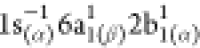 (at 402.80
eV) and
(at 402.80
eV) and  (at 403.33
eV), also called, in ref (85), the low- and high-energy
flanks of the 1sN → 2b1 resonance. However, we observed that the lower energy state is practically
dark, whereas the high energy state, calculated 403.33 eV, is bright:
the oscillator strengths obtained for the low- and high-energy flanks
are 2.6 × 10⁻⁴ and 6.6 × 10⁻², respectively. Therefore, we will concentrate only on the high energy
flank of the 1sN → 2b1 excitation in
the following analysis of the RAES of NO2. We note, nonetheless,
that, in the experimental analysis of Piancastelli et al.,85 as well as in the theoretical analysis of Grell
and Bokarev,68 the authors addressed the
effects of the different flanks of the 2b1 resonance to
the RAES, but their analyses were inconclusive, regarding the RAES
stemming from low-energy side of the resonance. Grell and Bokarev68 argued that resolving the RAES spectrum stemming
from the low energy state would require a more involved treatment
of the Auger decay process within the one-step model,70 as well as the inclusion of nuclear dynamics effects.
(at 403.33
eV), also called, in ref (85), the low- and high-energy
flanks of the 1sN → 2b1 resonance. However, we observed that the lower energy state is practically
dark, whereas the high energy state, calculated 403.33 eV, is bright:
the oscillator strengths obtained for the low- and high-energy flanks
are 2.6 × 10⁻⁴ and 6.6 × 10⁻², respectively. Therefore, we will concentrate only on the high energy
flank of the 1sN → 2b1 excitation in
the following analysis of the RAES of NO2. We note, nonetheless,
that, in the experimental analysis of Piancastelli et al.,85 as well as in the theoretical analysis of Grell
and Bokarev,68 the authors addressed the
effects of the different flanks of the 2b1 resonance to
the RAES, but their analyses were inconclusive, regarding the RAES
stemming from low-energy side of the resonance. Grell and Bokarev68 argued that resolving the RAES spectrum stemming
from the low energy state would require a more involved treatment
of the Auger decay process within the one-step model,70 as well as the inclusion of nuclear dynamics effects.
Figure 8.

NO2 RAES spectra at the N K-edge from OCA (blue) and SCI (orange). The experimental spectra were digitized from ref (85). The computed spectrum was broadened with Gaussian functions using a HWHM of 0.4 eV. The bottom panel shows the calculated and experimental PES (off resonance) spectrum to indicate the features in the RAES reminiscent from the PES.
The spectrum we obtained with the OCA-RASPT2 approach shows very
good agreement with the experimental data,85 as one can easily conclude by visual inspection of Figure 8. Therein, we also show the
stick spectrum of the peaks stemming from the singlet and triplet
states of NO2+. In contrast with what we observed
for HNCO, the triplet channels are the dominant states of the RAES
spectrum of NO2. The vertical solid gray lines shown in Figure 8 indicate the features
found in the PES spectrum that correspond to the  and 4
and 4 photoionizations, calculated at 18.8 and
20.9 eV, respectively. From the calculated PES (bottom panel of Figure 8), the general observation
is that all relevant features present in the experiment85 are reproduced by our calculation, implying
that our active space/basis set are well-suited for this problem.
A point of divergence from experiment is the intensity of the peak
observed at 20.9 eV
photoionizations, calculated at 18.8 and
20.9 eV, respectively. From the calculated PES (bottom panel of Figure 8), the general observation
is that all relevant features present in the experiment85 are reproduced by our calculation, implying
that our active space/basis set are well-suited for this problem.
A point of divergence from experiment is the intensity of the peak
observed at 20.9 eV  . Although
we reproduce the energy of this
state, its calculated intensity—obtained within the sudden
approximation114 limit—is underestimated.
The presence of the
. Although
we reproduce the energy of this
state, its calculated intensity—obtained within the sudden
approximation114 limit—is underestimated.
The presence of the  and
and  peaks in the experimental
RAES and their
absence in the calculated RAES spectrum suggest that a considerable
amount of the absorbed photon flux leads to direct ionization of the
molecule, instead of resonant excitation. This suggestion of direct
photoionized states being concomitantly generated with the RAES experimental
spectrum85 was originally put forward by
Grell and Bokarev,68 and we endorse it
here with our results.
peaks in the experimental
RAES and their
absence in the calculated RAES spectrum suggest that a considerable
amount of the absorbed photon flux leads to direct ionization of the
molecule, instead of resonant excitation. This suggestion of direct
photoionized states being concomitantly generated with the RAES experimental
spectrum85 was originally put forward by
Grell and Bokarev,68 and we endorse it
here with our results.
Moving to the analysis of the Auger spectrum,
we labeled the main
features observed in Figure 8 from 1 to 5. Feature 1 is a weak peak obtained at 10.7 eV,
and we assign it to the participator decay channel leading to the
cationic singlet state with configuration  —that is, the decay of the
  electron to fill the core–hole,
and the ejection of the core-excited electron in the 2b1 orbital into the continuum. Notice that this state can also be reached
by direct photoionization of the unpaired electron in the ground state
electron to fill the core–hole,
and the ejection of the core-excited electron in the 2b1 orbital into the continuum. Notice that this state can also be reached
by direct photoionization of the unpaired electron in the ground state  . The intense peak observed at ∼17
eV, labeled peak 2, is dominated by three triplet participator Auger
states, with major configurations
. The intense peak observed at ∼17
eV, labeled peak 2, is dominated by three triplet participator Auger
states, with major configurations  ,
,  , and
, and  , obtained at 17.2, 17.3, and 17.8
eV, respectively,
and by the singlet state with configuration
, obtained at 17.2, 17.3, and 17.8
eV, respectively,
and by the singlet state with configuration  , obtained at 17.7 eV. We also observe an
intense peak at 19.5 eV (peak 3) associated with the spectator
, obtained at 17.7 eV. We also observe an
intense peak at 19.5 eV (peak 3) associated with the spectator 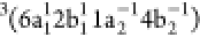 configuration,
followed by the intense
peak at 21.7 eV (peak 4) attributed to the spectator
configuration,
followed by the intense
peak at 21.7 eV (peak 4) attributed to the spectator  configuration.
The last feature we highlight
is peak 5, centered at 22.5 eV. This peak is associated with the overlap
of two triplet states assigned to the
configuration.
The last feature we highlight
is peak 5, centered at 22.5 eV. This peak is associated with the overlap
of two triplet states assigned to the  and
and 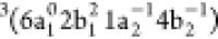 configurations.
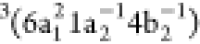
As expected, the results of OCA are in fairly good agreement with those of the SCI method. We highlight regions around peaks 2 and 3. In peak 2, the OCA intensity is more pronounced, whereas in peak 3, the SCI intensity is higher than the OCA. One can still see that the intensity of peak 1, which is a singlet decay channel, is practically the same in both methods. At higher energies (peaks 4 and 5), the decay rates are slightly larger in case of SCI. Similar to water, the differences are mostly stemming from the more pronounced contributions of triplet decay channels in the case of SCI.
4.7. Pyrimidine (C4H4N2)
We now benchmark our methodology against the experimental RAES of pyrimidine (C4H4N2), an organic molecule having four C and two N atoms arranged in a C2v symmetric six-membered heterocyclic ring. Since three nucleobases, thymine, cytosine and uracil, are pyrimidine derivatives, pyrimidine has been used as a common prototype system in numerous studies aimed at understanding the basics mechanisms involved in photoinduced DNA damage.86,115−121 We base our computational analysis on the recent XAS and RAES measurements at the N K-edge in the work of Bolognesi et al.86 A theoretical study has been recently reported for the XAS, RAES and PES of pyrimidine by Grell and Bokarev.68 In their report, the authors obtained resonant Auger spectra at the nitrogen K-edge based on the RASPT2 approximation level and the SCI.68 However, an overall agreement with the experimental RAES was not achieved; the authors tentatively assigned the observed inconsistencies to limitations in their quantum chemistry (QC) treatment of the initial and final bound states. With the aim of overcoming the above-mentioned disagreement between theory and experiment, here, we revisit the resonant Auger spectrum of pyrimidine at the N K-edge using new sets of RASPT2 calculations and two approximate treatments of the continuum, i.e., OCA and SCI.
For this purpose, we designed two different QC schemes in the following, which we reference as QC-I and QC-II, based on two distinct, but still compact, RAS spaces. A schematic representation of both QC schemes is shown in Figure 9.
Figure 9.

Restricted active spaces defining the quantum chemistry schemes QC-I and QC-II of pyrimidine. In the upper frame, we show scheme QC-I, which contains 10 orbitals and 14 electrons for the neutral system (13 electrons for the cation). In the lower frame, scheme QC-II is shown, which has 12 orbitals and 18 electrons for the neutral system (17 electrons for the cation).
In its ground state, considering C2v point-group symmetry, and the molecule lying on the xz-plane with the C2-axis along the z-direction, pyrimidine has the following HF configuration:
As noted previously, the RAS1 subspace is reserved for the 1sN orbitals. Notice that the 1sN orbitals displayed in Figure 9 are localized on each atomic center. For that purpose, and in a manner similar to what we did for N2, we reduced the point group symmetry in the calculations from C2v to Cs and localized the core orbitals applying a Cholesky localization procedure.95 The valence space is distributed differently in the two QC schemes. In QC-I, the set of molecular orbitals 11a1, 7b1, 1–3b2 and 1–3a2 was put in the RAS2 subspace, while the RAS3 subspace was kept empty. Thus, in QC-I, 14 active electrons are distributed over 10 active orbitals, restricted to a maximum of one hole in RAS1 and, as usual, a full CI treatment within the RAS2 space.122−124 To define QC-II, we moved the 3 π* orbitals into the RAS3 subspace, and added the set of occupied valence orbitals 10–11a1, 6–7b1, 1–2b2 and 1a2 to the RAS2 subspace. In QC-II, 18 active electrons are distributed over 12 orbitals restricted to a maximum of one hole in the RAS1 subspace and a maximum of two electrons in the RAS3 subspace. For the calculation of core-excited states, the CVS technique is invoked with the HEXS92 keyword available in OpenMolcas.72 In each QC scheme, cationic final (doublet) states have been obtained by state averaging over 150 states for each irreducible representation of the Cs point group.
Note that, in the SCI Auger calculation, the origin of the photoelectron orbital was set to the center of mass of the molecule (see section 3 for more computational details), whereas, in the OCA, the relevant matrix elements are projected onto a single N atom, similar to what we did for N2. Furthermore, the Auger-SCI code44,68 is not yet symmetry adapted, and therefore the RASSCF/RASPT2 calculations used with the SCI approach did not make use of point-group symmetry. On the other hand, the OCA scheme was implemented to take advantage of point group symmetry.
An analysis of the BEs obtained from the calculations with and without symmetry demonstrates only minute differences in the binding energies. Hence, employing point group symmetry is not mandatory, but simplifies (and accelerates) the bound-state calculations. The computational time spent in the SCI numerical continuum calculation for pyrimidine is also worth mentioning. The present SCI simulation was performed on 12 nodes/20 CPUs each (total of 240 CPUs) for ∼64 h. On the other hand, the OCA Auger decay rates are promptly obtained, their calculation taking no more than a few minutes on a single CPU, since the computational effort needed to project the MOs onto the MBS is minimal and the atomic two-electron integrals are simply tabulated numbers.
The 1sN → π*(2a2) core-excited energy of pyrimidine was calculated at 398.13 and 398.81 eV with QC-I and QC-II, respectively, whereas the measured reference value is 398.8 eV.86 Thus, both QC schemes reproduce the inner-shell excited state energy quite accurately. As for the resonant Auger, we start with the analysis of Figure 10a, where we compare the results obtained with the two continuum treatments, SCI and OCA, both based on the same QC-I scheme.
Figure 10.

Pyrimidine RAES spectra at the 1s → π*(2a2) resonance. The experimental spectrum was redigitized from ref (86). The computed spectra were broadened with Gaussian functions using a HWHM of 0.5 eV. On the left (panel (a)), we compare the spectra computed within the SCI and OCA continuum approximations, both based on QC-I scheme. On the right (panel (b)), the computed RAES obtained with the OCA and QC-II is compared to the experiment.
Visually, the convoluted spectra exhibit practically the same spectral
profiles, with only small differences. The Auger participator channels
associated with the final states with  , π–1(2b2),
  , and π–1(1a2) configurations appear in the low
energy region of the spectrum,
in increasing order of energy, from 9 to 11 eV (see data in Table 4). The calculated
participator states, from both SCI and OCA, resemble the experimental
profile quite well. The intensities (decay rates) are slightly larger
in the SCI, compared to the OCA spectrum, but the differences are
not substantial for any of the mentioned states. The remaining part
of the spectrum—above 12 eV—is dominated by a manifold
of spectator decay channels leading to cationic states with 2h1p character.
As we can observe, from the stick spectra plotted together with the
convoluted spectra, that multiple transition contribute to each peak,
making it difficult to assign the experimental features to a particular
orbital configuration. However, we do observe that the intensity distribution
in the entire region above 12 eV is not entirely satisfactory when
we compare both SCI and OCA QC-I results with the experiment. For
example, the relative intensity of the two peaks centered at ∼14.0
and 17.0 eV (peaks C and E in Table 4) are weaker than expected compared to the experimental
intensities, taking as reference, for comparison, the maximum of the
participator peak observed at ∼11 eV (peak B in Table 4).
, and π–1(1a2) configurations appear in the low
energy region of the spectrum,
in increasing order of energy, from 9 to 11 eV (see data in Table 4). The calculated
participator states, from both SCI and OCA, resemble the experimental
profile quite well. The intensities (decay rates) are slightly larger
in the SCI, compared to the OCA spectrum, but the differences are
not substantial for any of the mentioned states. The remaining part
of the spectrum—above 12 eV—is dominated by a manifold
of spectator decay channels leading to cationic states with 2h1p character.
As we can observe, from the stick spectra plotted together with the
convoluted spectra, that multiple transition contribute to each peak,
making it difficult to assign the experimental features to a particular
orbital configuration. However, we do observe that the intensity distribution
in the entire region above 12 eV is not entirely satisfactory when
we compare both SCI and OCA QC-I results with the experiment. For
example, the relative intensity of the two peaks centered at ∼14.0
and 17.0 eV (peaks C and E in Table 4) are weaker than expected compared to the experimental
intensities, taking as reference, for comparison, the maximum of the
participator peak observed at ∼11 eV (peak B in Table 4).
Table 4. Pyrimidine. Binding Energies and Main Character of Selected Cationic States of the RAES at the 1sN → π*(2a2) Resonance Computed with the QC-II Scheme (see Figure 9 for a Definition of the QC-I and QC-II Schemes)a.
| Binding
Energy, BE (eV) |
||||
|---|---|---|---|---|
| label | this work | experimentb | state main configuration [with CI weight]c | |
| A | 9.43 | 9.8 | ||
| 9.87 | 2b2–1[0.89] | |||
| B | 10.84 | 11.3 | ||
| 11.13 | 1a2–1[0.91] | |||
| C | 14.85 | 14.2 | ||
| D | 16.33 | ∼15.7 |
 [0.37] + [0.37] +  [0.19] [0.19] |
|
| E | 17.38 | 16.5 | ||
| 17.69 | 1a2–12b2–13b21[0.54] | |||
| 17.94 | ||||
| 18.17 | 11a1–17b1–12a21[0.49] | |||
| 18.23 |
 [0.41] + [0.41] +  [0.31] [0.31] |
|||
| F | 19.49 |
 [0.32] + [0.32] +  [0.20] [0.20] |
||
| 20.73 | 6b1–17b1–12a21[0.25] + 11a1–22a21[0.22] | |||
| 21.61 |
 [0.27] + [0.27] +  [0.14] [0.14] |
|||
| G | 24.61 | ∼25.8 |
 [0.12] + [0.12] +  [0.11] [0.11] |
|
The numbers in parentheses correspond to the CI weight of the respective configuration.
Data taken from ref (86).
Here, we show only configurations with CI weight of >0.1.
In an attempt to improve the intensity distribution of the RAES
in the second region of the spectrum, rich with spectator Auger decays,
we therefore computed the RAES with the OCA based on the QC-II scheme.
The spectrum computed with the QC-II scheme is presented in the top
panel of Figure 10b along, on the bottom panel, with the experimental spectrum measured
for the 1sN → π*(2a2) resonance.86 To help with the assignments, the main features
in the calculated spectrum are labeled from A to G, as in the experimental
spectrum.86 The same notation was used
in Table 4, where the
peaks assignments were based on the calculations performed with the
QC-II scheme. The analysis of the resonant Auger spectrum based on
QC-II is performed only for the OCA continuum, since its computational
cost is significantly less, compared to the SCI numerical procedure,
and since the comparison based on QC-I discussed earlier did not show
significant differences in the simulated spectra generated with the
SCI and OCA. The participator channels associated with the  , π–1(2b2),
  , and π–1(1a2) final states contribute to the peaks
labeled A and B (see Table 4 for the individual
BEs). These peaks got more intensity than previously obtained with
QC-I, but the convoluted shape of the overlapping peaks A and B is
the same as that observed previously.
, and π–1(1a2) final states contribute to the peaks
labeled A and B (see Table 4 for the individual
BEs). These peaks got more intensity than previously obtained with
QC-I, but the convoluted shape of the overlapping peaks A and B is
the same as that observed previously.
The main improvement brought
in with QC-II is indeed in the region
above 12 eV, rich in Auger spectator decays to 2h1p final cationic
states. The peak labeled C is assigned to the final state with main
configuration  and a BE of 14.85 eV. The most intense
peak seen from the experiment is peak E. Also, in the experiment,
we observe an asymmetry in the left side of peak E like a shoulder
near ∼15.7 eV. We suggest that this shoulder could be associated
with peak D obtained at 16.33 eV in the calculated spectrum. The cationic
final state associated with peak D has a multiconfigurational 2h1p
character, as it can be seen from the assignment in Table 4. In this final state, the holes
are distributed over the valence orbitals nN(7b1), nN(11a1),
π(1a2), π(2b2), and the particle
in the π*(2a2) virtual orbital. The intense peak
E overlaps with a large number of transitions, and the most intense
ones are listed in Table 4. However, notice that the intensity at the maximum of peak
E, when compared to peak B, is more in accord with the experimental
profile than that observed for QC-I. The center of peak E in the convoluted
spectrum is red-shifted by ∼1 eV, with respect to the experiment.
This error can be immediately attributed to the limitations in our
quantum chemistry approximation, even though we cannot discard photodissociation
or other nuclear dynamical effects, which are ignored in our simulations.
It is known that the RAES is very sensitive to nuclear relaxation
processes.11−14,63,64,66 The inclusion of nuclear dynamic effects
will be addressed in a further extension of this work aimed at time-resolved
Auger simulations. For the moment, we retain ourselves to the analysis
of the Auger spectra with the static ground-state equilibrium geometry.
Furthermore, the region of the spectrum labeled F also comprises a
very large number of transitions. We highlight the shakeup 2h1p state calculated at 19.49 eV in which the particle is observed
in the π*(3b2) virtual orbital instead of the π*(2a2). Following peak F, a weak peak is observed at ∼25
eV, which we label as peak G. According to our assignment, given in Table 4, the holes in the
cationic 2h1p final state associated with peak G are distributed over
the valence orbitals nN(6b1) and nN(10a1), and the particle
in the virtual orbitals π*(2a2) and π*(3b2).
and a BE of 14.85 eV. The most intense
peak seen from the experiment is peak E. Also, in the experiment,
we observe an asymmetry in the left side of peak E like a shoulder
near ∼15.7 eV. We suggest that this shoulder could be associated
with peak D obtained at 16.33 eV in the calculated spectrum. The cationic
final state associated with peak D has a multiconfigurational 2h1p
character, as it can be seen from the assignment in Table 4. In this final state, the holes
are distributed over the valence orbitals nN(7b1), nN(11a1),
π(1a2), π(2b2), and the particle
in the π*(2a2) virtual orbital. The intense peak
E overlaps with a large number of transitions, and the most intense
ones are listed in Table 4. However, notice that the intensity at the maximum of peak
E, when compared to peak B, is more in accord with the experimental
profile than that observed for QC-I. The center of peak E in the convoluted
spectrum is red-shifted by ∼1 eV, with respect to the experiment.
This error can be immediately attributed to the limitations in our
quantum chemistry approximation, even though we cannot discard photodissociation
or other nuclear dynamical effects, which are ignored in our simulations.
It is known that the RAES is very sensitive to nuclear relaxation
processes.11−14,63,64,66 The inclusion of nuclear dynamic effects
will be addressed in a further extension of this work aimed at time-resolved
Auger simulations. For the moment, we retain ourselves to the analysis
of the Auger spectra with the static ground-state equilibrium geometry.
Furthermore, the region of the spectrum labeled F also comprises a
very large number of transitions. We highlight the shakeup 2h1p state calculated at 19.49 eV in which the particle is observed
in the π*(3b2) virtual orbital instead of the π*(2a2). Following peak F, a weak peak is observed at ∼25
eV, which we label as peak G. According to our assignment, given in Table 4, the holes in the
cationic 2h1p final state associated with peak G are distributed over
the valence orbitals nN(6b1) and nN(10a1), and the particle
in the virtual orbitals π*(2a2) and π*(3b2).
5. Summary and Outlook
We have presented RAES and AES spectra obtained with a new implementation of the Auger decay rates using the one-center approximation48,49,53,125 based on a RASSCF/RASPT2 description of the target initial and ionized final states. Our implementation in OpenMolcas takes advantage of the Abelian point group symmetry, which usually simplifies the calculations and the analysis of the final results. Furthermore, a straightforward recipe was presented to select, from the cc-pVXZ family76,90 of contracted basis sets, a minimal basis set onto which we project the original MOs. This recipe can be easily extended to any other family of contracted basis sets. Resonant and nonresonant Auger spectra were obtained in very good agreement with experimental data for neon, carbon monoxide, molecular nitrogen, isocyanic acid, water, nitrogen dioxide, and pyrimidine. For nitrogen dioxide and pyrimidine, arguably the most challenging molecular systems in this work due to the open-shell doublet ground state in the first case and the molecular size in the other, the Auger spectra obtained with both the OCA and the Auger-SCI approach44,68 yielded very similar results.
Our first showcase system was the 1s → 3p core-excited Ne atom, whose resonant Auger spectrum stems almost entirely from spectator and shakeup decay channels. The latter involves a promotion to a Rydberg level, that is, its final states take the form (2s2p)64p1. These shakeup Ne+ states have a tendency to be very sensitive to the presence of diffuse primitives in the basis set.44 Thus, for the Ne atom, we used a modified d-aug-cc-pVQZ basis90 augmented with (3s2p2d) Rydberg-like functions.91 For the remaining molecular systems, we used compact basis sets—such as cc-pVTZ or a combination of DZ with TZ—since we were not aiming at the involvement of Rydberg states in the decay channels of molecular systems, but instead, in reproducing the main features observed in the experiments maintaining a good compromise between quality and computational cost.
Furthermore, we analyzed the resonant and nonresonant Auger spectra of the small molecules CO, N2, HNCO, and H2O, which have been previously computed within the OCA elsewhere46,48,53,82,84 mostly based on CASCI initial and final state wave functions, which are lacking dynamical correlation. Our calculations differ mainly in the inclusion of dynamical correlation effects on the initial and final state wave functions by means of the MS-RASPT2 approximation,57,58 and electronic relaxation of the core excited/ionized states by use of a set of biorthogonal bound orbitals obtained within the SI approach.59,74 The Auger spectra of CO and N2 obtained here are very similar to previous results reported by Fink and co-workers.48,53,82 For the isocyanic acid, correlation effects are apparently more relevant in the calculations of initial core-excited and the final cationic states, as we observe better agreement between experiment and our calculated spectra than in previously reported calculations,84 without having to rescale the BEs with an empirical factor.
Being an open-shell system, the 1sN → π*(2b1) core-excited NO2 molecule can decay either to singlets or triplets NO2+ final states. We have demonstrated that, different from the normal Auger spectrum of isocyanic acid, the triplet decay channels of NO2 are responsible for the most intense transitions of the resonant Auger spectrum.85 The decay rates obtained from the OCA and SCI continuum approximations have been obtained in very good agreement with each other and also with a former computational study solely based on the SCI continuum method.68
For the pyrimidine molecule, the resonant Auger spectra obtained with the two distinct continuum approximations—OCA and SCI, based on the same RASPT2 space selection (labeled QC-I scheme)—yielded very similar profiles. This an important point, since the SCI method is conceivably more accurate than the OCA, because it accounts for the ionic potential (in a spherically averaged way) with the multicenter two-electron bound-continuum integrals explicitly computed, whereas in the OCA these integrals are reduced to a single center quantity. Moreover, the computational time spent in the SCI approximation is substantially longer than needed for the simpler OCA. This is an important aspect one must take into consideration if aiming at practical simulations of time-resolved Auger spectra for example, where, in a trajectory-based dynamics, a large number of Auger spectra must be computed on the fly.126,127 Another important aspect, when using the Auger-SCI approach,44,68 is the necessity to interface the bound state quantities obtained within OpenMolcas with the external code that performs the numerical continuum calculation. On the other hand, an Auger spectrum can be obtained straightaway from OpenMolcas with the OCA, eliminating the extra burden of interfacing between different codes. We have shown with the calculations based on the QC-II scheme that the resonant Auger spectrum of pyrimidine can be calculated with very reasonable agreement with the experimental data86 by using a rather small basis set combined with a still compact (and accessible) restricted active space.
Aside from all its favorable characteristics, one also must beware of the possible limitations when applying the OCA to a general molecular system (or a cluster). One of them is associated with the fact that the OCA neglects scattering effects from the noncore-hole atoms, affecting the angular expansion of the continuum channels,54 and possibly the computed Auger intensities. Moreover, only a few attempts have been made to use the OCA in molecules of the size and complexity of pyrimidine.67 This might be related with difficulties in dealing with resonances arising from delocalized core-holes over several equivalent atoms (plus, of course, the challenges in defining good and compact RASSCF spaces for large molecules). For two cases presented here, N2 and C4N2H4, the N 1s orbitals are delocalized over two equivalent atomic centers. Nonetheless, we could (with the Cholesky approach95) localize the core and use the fact that the N atoms in those molecules are symmetrically equivalent, so the one-center approximation could be employed without significant loss of accuracy. The same strategy could be easily applied, for example, to compute the Auger spectra at the oxygen K-edges of NO2 or CO2. The applicability of the OCA to the carbon K-edge of C4N2H4, for example, is maybe less clear, because of the large number of C K-edge sites. However, using a localization procedure similar to the one here applied for the N K-edge, it should still be possible to obtain satisfactory Auger spectra at the C K-edge by an incoherent sum over intensities for each atom (i.e., each core hole). The extent by which the OCA-RASPT2 approach may be applied and its performance to obtain the Auger spectra of systems with more than two equivalent core holes is granted and will be the subject of future investigation. Furthermore, we plan to explore the applicability of our OCA-RASPT2 approach coupled to nuclear dynamics for time-resolved studies of complex molecules.
Acknowledgments
We would like to thank Dr. Gilbert Grell for the SCAMPI code and his assistance in its application. This work was performed with support from the European Union’s Horizon 2020 Research and Innovation Programme under the Marie Skłodowska-Curie Individual Fellowship (B.N.C.T., Grant Agreement No. 101027796), from the Independent Research Fund Denmark–Natural Sciences, DFF-RP2 Grant No. 7014-00258B (S.C.), from the Research Council of Norway through FRINATEK (Project No. 275506), Theolight (S.C.), and from the Deutsche Forschungsgemeinschaft (Grant No. BO 4915/1-1) (S.I.B.). The European Cooperation in Science and Technology, COST Action CA18222, Attochem, is also acknowledged.
Supporting Information Available
The Supporting Information is available free of charge at https://pubs.acs.org/doi/10.1021/acs.jctc.2c00252.
Total decay rates and number of basis functions for each molecule; schematic illustrations of the procedure adopted to select the minimal basis sets (MBS) for oxygen and neon; optimized structure of pyrimidine (Cartesian coordinates) (PDF)
The authors declare no competing financial interest.
Supplementary Material
References
- Hofmann S. In Auger- and X-Ray Photoelectron Spectroscopy in Materials Science; Ertl G., Lüth H., Mills D. L., Eds.; Springer Series in Surface Sciences; Springer: Berlin, Heidelberg, 2013. [Google Scholar]
- Svensson S. Soft x-ray photoionization of atoms and molecules. J. Phys. B-At. Mol. Opt. 2005, 38, S821–S838. 10.1088/0953-4075/38/9/024. [DOI] [Google Scholar]
- Armen G. B.; Aksela H.; Åberg T.; Aksela S. The resonant Auger effect. J. Phys. B-At. Mol. Opt. 2000, 33, R49–R92. 10.1088/0953-4075/33/2/201. [DOI] [Google Scholar]
- Ågren H.; Cesar A.; Liegener C.-M. In Theory of Molecular Auger Spectra; Löwdin P.-O., Sabin J. R., Zerner M. C., Eds.; Advances in Quantum Chemistry, Vol. 23; Academic Press, 1992; pp 1–82. [Google Scholar]
- Nicolas C.; Miron C. Lifetime broadening of core-excited and -ionized states. J. Electron Spectrosc. Relat. Phenom. 2012, 185, 267–272. 10.1016/j.elspec.2012.05.008. [DOI] [Google Scholar]
- Travnikova O.; Sisourat N.; Marchenko T.; Goldsztejn G.; Guillemin R.; Journel L.; Céolin D.; Ismail I.; Lago A. F.; Püttner R.; Piancastelli M. N.; Simon M. Subfemtosecond Control of Molecular Fragmentation by Hard X-Ray Photons. Phys. Rev. Lett. 2017, 118, 213001. 10.1103/PhysRevLett.118.213001. [DOI] [PubMed] [Google Scholar]
- Tenorio B. N. C.; Ponzi A.; Coriani S.; Decleva P. Photoionization Observables from Multi-Reference Dyson Orbitals Coupled to B-Spline DFT and TD-DFT Continuum. Molecules 2022, 27, 1203. 10.3390/molecules27041203. [DOI] [PMC free article] [PubMed] [Google Scholar]
- Cederbaum L. S.; Zobeley J.; Tarantelli F. Giant Intermolecular Decay and Fragmentation of Clusters. Phys. Rev. Lett. 1997, 79, 4778–4781. 10.1103/PhysRevLett.79.4778. [DOI] [Google Scholar]
- Averbukh V.; Cederbaum L. S. Ab initio calculation of interatomic decay rates by a combination of the Fano ansatz, Green’s-function methods, and the Stieltjes imaging technique. J. Chem. Phys. 2005, 123, 204107. 10.1063/1.2126976. [DOI] [PubMed] [Google Scholar]
- Zobeley J.; Santra R.; Cederbaum L. S. Electronic decay in weakly bound heteroclusters: Energy transfer versus electron transfer. J. Chem. Phys. 2001, 115, 5076–5088. 10.1063/1.1395555. [DOI] [Google Scholar]
- Gessner O.; Gühr M. Monitoring Ultrafast Chemical Dynamics by Time-Domain X-ray Photo- and Auger-Electron Spectroscopy. Acc. Chem. Res. 2016, 49, 138–145. 10.1021/acs.accounts.5b00361. [DOI] [PubMed] [Google Scholar]
- McFarland B. K.; Farrell J. P.; Miyabe S.; Tarantelli F.; Aguilar A.; Berrah N.; Bostedt C.; Bozek J. D.; Bucksbaum P. H.; Castagna J. C.; Coffee R. N.; Cryan J. P.; Fang L.; Feifel R.; Gaffney K. J.; Glownia J. M.; Martinez T. J.; Mucke M.; Murphy B.; Natan A.; Osipov T.; Petrović V. S.; Schorb S.; Schultz T.; Spector L. S.; Swiggers M.; Tenney I.; Wang S.; White J. L.; White W.; Gühr M. Ultrafast X-ray Auger probing of photoexcited molecular dynamics. Nat. Commun. 2014, 5, 4235. 10.1038/ncomms5235. [DOI] [PubMed] [Google Scholar]
- Wolf T. J. A.; Paul A. C.; Folkestad S. D.; Myhre R. H.; Cryan J. P.; Berrah N.; Bucksbaum P. H.; Coriani S.; Coslovich G.; Feifel R.; Martinez T. J.; Moeller S. P.; Mucke M.; Obaid R.; Plekan O.; Squibb R. J.; Koch H.; Gühr M. Transient resonant Auger–Meitner spectra of photoexcited thymine. Faraday Discuss. 2021, 228, 555–570. 10.1039/D0FD00112K. [DOI] [PubMed] [Google Scholar]
- Lever F.; Mayer D.; Metje J.; Alisauskas S.; Calegari F.; Düsterer S.; Feifel R.; Niebuhr M.; Manschwetus B.; Kuhlmann M.; Mazza T.; Robinson M. S.; Squibb R. J.; Trabattoni A.; Wallner M.; Wolf T. J. A.; Gühr M. Core-Level Spectroscopy of 2-Thiouracil at the Sulfur L1- and L2,3-Edges Utilizing a SASE Free-Electron Laser. Molecules 2021, 26, 6469. 10.3390/molecules26216469. [DOI] [PMC free article] [PubMed] [Google Scholar]
- Travnikova O.; Kukk E.; Hosseini F.; Granroth S.; Itälä E.; Marchenko T.; Guillemin R.; Ismail I.; Moussaoui R.; Journel L.; Bozek J.; Püttner R.; Krasnov P. O.; Kimberg V.; Gel’mukhanov F.; Piancastelli M. N.; Simon M. Ultrafast dissociation of ammonia: Auger Doppler effect and redistribution of the internal energy. Phys. Chem. Chem. Phys. 2022, 24, 5842–5854. 10.1039/D1CP05499F. [DOI] [PubMed] [Google Scholar]
- Coutinho L. H.; de A. Ribeiro F.; Tenorio B. N. C.; Coriani S.; dos Santos A. C. F.; Nicolas C.; Milosavljevic A. R.; Bozek J. D.; Wolff W. NEXAFS and MS-AES spectroscopy of the C 1s and Cl 2p excitation and ionization of chlorobenzene: Production of dicationic species. Phys. Chem. Chem. Phys. 2021, 23, 27484–27497. 10.1039/D1CP03121J. [DOI] [PubMed] [Google Scholar]
- Travnikova O.; Marchenko T.; Goldsztejn G.; Jänkälä K.; Sisourat N.; Carniato S.; Guillemin R.; Journel L.; Céolin D.; Püttner R.; Iwayama H.; Shigemasa E.; Piancastelli M. N.; Simon M. Hard-X-Ray-Induced Multistep Ultrafast Dissociation. Phys. Rev. Lett. 2016, 116, 213001. 10.1103/PhysRevLett.116.213001. [DOI] [PubMed] [Google Scholar]
- Santos A. C. F.; Vasconcelos D. N.; MacDonald M. A.; Sant’Anna M. M.; Tenório B. N. C.; Rocha A. B.; Morcelle V.; Appathurai N.; Zuin L. Atomic versus molecular Auger decay in CH2Cl2 and CD2Cl2 molecules. J. Chem. Phys. 2018, 149, 054303. 10.1063/1.5030644. [DOI] [PubMed] [Google Scholar]
- Santos A. C. F.; Vasconcelos D. N.; MacDonald M. A.; Sant’Anna M. M.; Tenório B. N. C.; Rocha A. B.; Morcelle V.; Bonfim V. S.; Appathurai N.; Zuin L. Evidence of ultrafast dissociation in the CHCl3 molecule. J. Phys. B-At. Mol. Opt. 2021, 54, 015202. 10.1088/1361-6455/abc9cc. [DOI] [Google Scholar]
- Goldsztejn G.; Guillemin R.; Marchenko T.; Travnikova O.; Ceolin D.; Journel L.; Simon M.; Piancastelli M. N.; Püttner R. Simulation of Auger decay dynamics in the hard x-ray regime: HCl as showcase. Phys. Chem. Chem. Phys. 2022, 24, 6590–6604. 10.1039/D1CP05662J. [DOI] [PubMed] [Google Scholar]
- Langhoff P. W.; Langhoff S. R.; Rescigno T. N.; Schirmer J.; Cederbaum L. S.; Domcke W.; Von Niessen W. Theoretical studies of inner-valence-shell photoionization cross sections in N2 and CO. Chem. Phys. 1981, 58, 71–91. 10.1016/0301-0104(81)80047-X. [DOI] [Google Scholar]
- Padial N.; Csanak G.; McKoy B. V.; Langhoff P. W. Photoabsorption in carbon monoxide: Stieltjes–Tchebycheff calculations in the separated-channel static-exchange approximation. J. Chem. Phys. 1978, 69, 2992–3004. 10.1063/1.437017. [DOI] [Google Scholar]
- Müller-Plathe F.; Diercksen G. H. In Electronic Structure of Atoms, Molecules and Solids. Proceeding of the II Escola Brasileira de Estructure Eletronica, Olinda, Brazil, July 17–22, 1989; Canuto S., D’Albuquerque e Castro J., Paixao F. J., Eds.; World Scientific: Olinda, Brazil, 1990; pp 1–29. [Google Scholar]
- Gokhberg K.; Vysotskiy V.; Cederbaum L. S.; Storchi L.; Tarantelli F.; Averbukh V. Molecular photoionization cross sections by Stieltjes-Chebyshev moment theory applied to Lanczos pseudospectra. J. Chem. Phys. 2009, 130, 064104. 10.1063/1.3073821. [DOI] [PubMed] [Google Scholar]
- Carravetta V.; Ågren H. In Computational Strategies for Spectroscopy: From Small Molecules to Nano Systems; Barone V., Ed.; John Wiley & Sons: Hoboken, NJ, 2012; pp 137–205. [Google Scholar]
- Moitra T.; Coriani S.; Cabral Tenorio B. N. Inner-shell photoabsorption and photoionisation cross-sections of valence excited states from asymmetric-Lanczos equation-of-motion coupled cluster singles and doubles theory. Mol. Phys. 2021, 119, e1980235 10.1080/00268976.2021.1980235. [DOI] [Google Scholar]
- Tenorio B. N. C.; Coriani S.; Rocha A. B.; Nascimento M. A. C. In Molecular Photoionization and Photodetachment Cross Sections Based on L2 Basis Sets: Theory and Selected Examples; Glushkov A. V., Khetselius O. Y., Maruani J., Brändas E., Eds.; Advances in Methods and Applications of Quantum Systems in Chemistry, Physics, and Biology; Springer International Publishing: Cham, Switzerland, 2021; pp 151–179. [Google Scholar]
- Tenorio B. N. C.; Nascimento M. A. C.; Coriani S.; Rocha A. B. Coupled Cluster Study of Photoionization and Photodetachment Cross Sections. J. Chem. Theory Comp. 2016, 12, 4440–4459. 10.1021/acs.jctc.6b00524. [DOI] [PubMed] [Google Scholar]
- Tenorio B. N. C.; Moitra T.; Nascimento M. A. C.; Rocha A. B.; Coriani S. Molecular inner-shell photoabsorption/photoionization cross sections at core-valence-separated coupled cluster level: Theory and examples. J. Chem. Phys. 2019, 150, 224104. 10.1063/1.5096777. [DOI] [PubMed] [Google Scholar]
- Cabral Tenorio B. N.; Chaer Nascimento M. A.; Rocha A. B. X-ray Photoionization Cross Section Spectra of Water and Ammonia Bonded on Polycyclic Aromatic Hydrocarbons: A Quantum Mechanical Interpretation to the Absorption Spectra on Graphene. J. Phys. Chem. A 2020, 124, 2591–2600. 10.1021/acs.jpca.9b11406. [DOI] [PubMed] [Google Scholar]
- Kopelke S.; Gokhberg K.; Cederbaum L. S.; Tarantelli F.; Averbukh V. Autoionization widths by Stieltjes imaging applied to Lanczos pseudospectra. J. Chem. Phys. 2011, 134, 024106. 10.1063/1.3523982. [DOI] [PubMed] [Google Scholar]
- Bachau H.; Cormier E.; Decleva P.; Hansen J. E.; Martín F. Applications of B-splines in atomic and molecular physics. Rep. Prog. Phys. 2001, 64, 1815–1943. 10.1088/0034-4885/64/12/205. [DOI] [Google Scholar]
- Brosolo M.; Decleva P.; Lisini A. LCAO expansion in a spline basis for accurate variational determination of continuum wavefunctions. Applications to H2+ and HeH2+. Chem. Phys. 1994, 181, 85–95. 10.1016/0301-0104(94)85017-8. [DOI] [Google Scholar]
- Ponzi A.; Angeli C.; Cimiraglia R.; Coriani S.; Decleva P. Dynamical photoionization observables of the CS molecule: The role of electron correlation. J. Chem. Phys. 2014, 140, 204304. 10.1063/1.4876495. [DOI] [PubMed] [Google Scholar]
- Ponzi A.; Quadri N.; Angeli C.; Decleva P. Electron correlation effects in the photoionization of CO and isoelectronic diatomic molecules. Phys. Chem. Chem. Phys. 2019, 21, 1937–1951. 10.1039/C8CP06103C. [DOI] [PubMed] [Google Scholar]
- Moitra T.; Ponzi A.; Koch H.; Coriani S.; Decleva P. Accurate Description of Photoionization Dynamical Parameters. J. Phys. Chem. Lett. 2020, 11, 5330–5337. 10.1021/acs.jpclett.0c01337. [DOI] [PubMed] [Google Scholar]
- Moitra T.; Coriani S.; Decleva P. Capturing Correlation Effects on Photoionization Dynamics. J. Chem. Theory Comput. 2021, 17, 5064–5079. 10.1021/acs.jctc.1c00303. [DOI] [PubMed] [Google Scholar]
- Carravetta V.; Ågren H. Stieltjes imaging method for molecular Auger transition rates: Application to the Auger spectrum of water. Phys. Rev. A 1987, 35, 1022–1032. 10.1103/PhysRevA.35.1022. [DOI] [PubMed] [Google Scholar]
- Kolorenč P.; Averbukh V. K-shell Auger lifetime variation in doubly ionized Ne and first row hydrides. J. Chem. Phys. 2011, 135, 134314. 10.1063/1.3646204. [DOI] [PubMed] [Google Scholar]
- Skomorowski W.; Krylov A. I. Feshbach-Fano approach for calculation of Auger decay rates using equation-of-motion coupled-cluster wave functions. I. Theory and implementation. J. Chem. Phys. 2021, 154, 084124. 10.1063/5.0036976. [DOI] [PubMed] [Google Scholar]
- Skomorowski W.; Krylov A. I. Feshbach–Fano approach for calculation of Auger decay rates using equation-of-motion coupled-cluster wave functions. II. Numerical examples and benchmarks. J. Chem. Phys. 2021, 154, 084125. 10.1063/5.0036977. [DOI] [PubMed] [Google Scholar]
- Colle R.; Simonucci S. Method for calculating Auger decay rates in molecules. Phys. Rev. A 1989, 39, 6247–6258. 10.1103/PhysRevA.39.6247. [DOI] [PubMed] [Google Scholar]
- Schimmelpfennig B.; Nestmann B. M.; Peyerimhoff S. D. Ab initio calculation of transition rates for autoionization: the Auger spectra of HF and F–. J. Electron Spectrosc. Relat. Phenom. 1995, 74, 173–186. 10.1016/0368-2048(95)02373-9. [DOI] [Google Scholar]
- Grell G.; Kühn O.; Bokarev S. I. Multireference quantum chemistry protocol for simulating autoionization spectra: Test of ionization continuum models for the neon atom. Phys. Rev. A 2019, 100, 042512. 10.1103/PhysRevA.100.042512. [DOI] [Google Scholar]
- Inhester L.; Burmeister C. F.; Groenhof G.; Grubmüller H. Auger spectrum of a water molecule after single and double core ionization. J. Chem. Phys. 2012, 136, 144304. 10.1063/1.3700233. [DOI] [PubMed] [Google Scholar]
- Siegbahn H.; Asplund L.; Kelfve P. The Auger electron spectrum of water vapour. Chem. Phys. Lett. 1975, 35, 330–335. 10.1016/0009-2614(75)85615-6. [DOI] [Google Scholar]
- Freund H.; Llegener C. Autoionization of CO after C 1s → 2π* excitation: a comparison with photoemission and auger decay. Chem. Phys. Lett. 1987, 134, 70–75. 10.1016/0009-2614(87)80016-7. [DOI] [Google Scholar]
- Fink R. Theoretical autoionization spectra of 1s → π* excited N2 and N2O. J. Electron Spectrosc. Relat. Phenom. 1995, 76, 295–300. 10.1016/0368-2048(95)02469-7. [DOI] [Google Scholar]
- Fink R. A theoretical simulation of the 1s → 2π excitation and deexcitation spectra of the NO molecule. J. Chem. Phys. 1997, 106, 4038–4052. 10.1063/1.473137. [DOI] [Google Scholar]
- Ohrendorf E. M.; Tarantelli F.; Cederbaum L. S. Dicationic states of hydrocarbons and a statistical approach to their Auger spectra. J. Chem. Phys. 1990, 92, 2984–2999. 10.1063/1.457894. [DOI] [Google Scholar]
- Minelli D.; Tarantelli F.; Sgamellotti A.; Cederbaum L. S. Theoretical simulation of molecular Auger spectra: The carbon and oxygen KLL Auger spectra of formaldehyde. J. Chem. Phys. 1993, 99, 6688–6696. 10.1063/1.465859. [DOI] [Google Scholar]
- Mitani M.; Takahashi O.; Saito K.; Iwata S. Theoretical molecular Auger spectra with electron population analysis. J. Electron Spectrosc. Relat. Phenom. 2003, 128, 103–117. 10.1016/S0368-2048(02)00270-0. [DOI] [Google Scholar]
- Kukk E.; Bozek J. D.; Cheng W.-T.; Fink R. F.; Wills A. A.; Berrah N. Auger decay of the C 1s → 2π* resonance in carbon monoxide: Vibrationally and angularly resolved spectra. J. Chem. Phys. 1999, 111, 9642–9650. 10.1063/1.480337. [DOI] [Google Scholar]
- Fink R. F.; Piancastelli M. N.; Grum-Grzhimailo A. N.; Ueda K. Angular distribution of Auger electrons from fixed-in-space and rotating C1s → 2π photoexcited CO: Theory. J. Chem. Phys. 2009, 130, 014306. 10.1063/1.3042153. [DOI] [PubMed] [Google Scholar]
- Andersson K.; Malmqvist P.-Å.; Roos B. O.; Sadlej A. J.; Wolinski K. Second-order perturbation theory with a CASSCF reference function. J. Phys. Chem. 1990, 94, 5483–5488. 10.1021/j100377a012. [DOI] [Google Scholar]
- Andersson K.; Malmqvist P.; Roos B. O. Second-order perturbation theory with a complete active space self-consistent field reference function. J. Chem. Phys. 1992, 96, 1218–1226. 10.1063/1.462209. [DOI] [Google Scholar]
- Malmqvist P.-Å.; Pierloot K.; Shahi A. R. M.; Cramer C. J.; Gagliardi L. The restricted active space followed by second-order perturbation theory method: Theory and application to the study of CuO2 and Cu2O2 systems. J. Chem. Phys. 2008, 128, 204109. 10.1063/1.2920188. [DOI] [PubMed] [Google Scholar]
- Sauri V.; Serrano-Andrés L.; Shahi A. R. M.; Gagliardi L.; Vancoillie S.; Pierloot K. Multiconfigurational Second-Order Perturbation Theory Restricted Active Space (RASPT2) Method for Electronic Excited States: A Benchmark Study. J. Chem. Theory Comput. 2011, 7, 153–168. 10.1021/ct100478d. [DOI] [PubMed] [Google Scholar]
- Malmqvist P.-Å.; Roos B. O. The CASSCF state interaction method. Chem. Phys. Lett. 1989, 155, 189–194. 10.1016/0009-2614(89)85347-3. [DOI] [Google Scholar]
- Geng T.; Ehrmaier J.; Schalk O.; Richings G. W.; Hansson T.; Worth G.; Thomas R. D. Time-Resolved Photoelectron Spectroscopy Studies of Isoxazole and Oxazole. J. Phys. Chem. A 2020, 124, 3984–3992. 10.1021/acs.jpca.9b11788. [DOI] [PMC free article] [PubMed] [Google Scholar]
- Berrah N.; Fang L.; Murphy B.; Osipov T.; Ueda K.; Kukk E.; Feifel R.; van der Meulen P.; Salen P.; Schmidt H. T.; Thomas R. D.; Larsson M.; Richter R.; Prince K. C.; Bozek J. D.; Bostedt C.; Wada S.-i.; Piancastelli M. N.; Tashiro M.; Ehara M. Double-core-hole spectroscopy for chemical analysis with an intense X-ray femtosecond laser. Proc. Natl. Acad. Sci. U. S. A. 2011, 108, 16912–16915. 10.1073/pnas.1111380108. [DOI] [PMC free article] [PubMed] [Google Scholar]
- Zhaunerchyk V.; Mucke M.; Salén P.; vd Meulen P.; Kaminska M.; Squibb R. J.; Frasinski L. J.; Siano M.; Eland J. H. D.; Linusson P.; et al. Using covariance mapping to investigate the dynamics of multi-photon ionization processes of Ne atoms exposed to X-FEL pulses. J. Phys. B: At. Mol. Opt. Phys. 2013, 46, 164034. 10.1088/0953-4075/46/16/164034. [DOI] [Google Scholar]
- Bao Z.; Fink R. F.; Travnikova O.; Céolin D.; Svensson S.; Piancastelli M. N. Detailed theoretical and experimental description of normal Auger decay in O2. J. Phys. B-At. Mol. Opt. 2008, 41, 125101. 10.1088/0953-4075/41/12/125101. [DOI] [Google Scholar]
- Takahashi O.; Odelius M.; Nordlund D.; Nilsson A.; Bluhm H.; Pettersson L. G. M. Auger decay calculations with core-hole excited-state molecular-dynamics simulations of water. J. Chem. Phys. 2006, 124, 064307. 10.1063/1.2166234. [DOI] [PubMed] [Google Scholar]
- Hjelte I.; Piancastelli M.; Fink R.; Björneholm O.; Bässler M.; Feifel R.; Giertz A.; Wang H.; Wiesner K.; Ausmees A.; Miron C.; Sorensen S.; Svensson S. Evidence for ultra-fast dissociation of molecular water from resonant Auger spectroscopy. Chem. Phys. Lett. 2001, 334, 151–158. 10.1016/S0009-2614(00)01434-2. [DOI] [Google Scholar]
- Eroms M.; Vendrell O.; Jungen M.; Meyer H.-D.; Cederbaum L. S. Nuclear dynamics during the resonant Auger decay of water molecules. J. Chem. Phys. 2009, 130, 154307. 10.1063/1.3117902. [DOI] [PubMed] [Google Scholar]
- Inhester L.; Oostenrijk B.; Patanen M.; Kokkonen E.; Southworth S. H.; Bostedt C.; Travnikova O.; Marchenko T.; Son S.-K.; Santra R.; Simon M.; Young L.; Sorensen S. L. Chemical Understanding of the Limited Site-Specificity in Molecular Inner-Shell Photofragmentation. J. Phys. Chem. Lett. 2018, 9, 1156–1163. 10.1021/acs.jpclett.7b03235. [DOI] [PubMed] [Google Scholar]
- Grell G.; Bokarev S. I. Multi-reference protocol for (auto)ionization spectra: Application to molecules. J. Chem. Phys. 2020, 152, 074108. 10.1063/1.5142251. [DOI] [PubMed] [Google Scholar]
- Wentzel G. Über strahlungslose Quantensprünge. Zeitschrift für Physik 1927, 43, 524–530. 10.1007/BF01397631. [DOI] [Google Scholar]
- Åberg T.; Howat G. In Encyclopedia of Physics, Vol. 31; Mehlhorn W., Ed.; Springer: Berlin, 1982; pp 469–619. [Google Scholar]
- Manne R.; Ågren H. Auger transition amplitudes from general many-electron wavefunctions. Chem. Phys. 1985, 93, 201–208. 10.1016/0301-0104(85)80018-5. [DOI] [Google Scholar]
- Fdez. Galván I.; Vacher M.; Alavi A.; Angeli C.; Aquilante F.; Autschbach J.; Bao J. J.; Bokarev S. I.; Bogdanov N. A.; Carlson R. K.; et al. OpenMolcas: From Source Code to Insight. J. Chem. Theory Comput. 2019, 15, 5925–5964. 10.1021/acs.jctc.9b00532. [DOI] [PubMed] [Google Scholar]
- OpenMolcas Project. Available via the Internet at: https://gitlab.com/Molcas/OpenMolcas (accessed June 6, 2022).
- Malmqvist P. Å. Calculation of transition density matrices by nonunitary orbital transformations. Int. J. Quantum Chem. 1986, 30, 479–494. 10.1002/qua.560300404. [DOI] [Google Scholar]
- Tenorio B. N. C.; Decleva P.; Coriani S. Multi-reference approach to the computation of double core-hole spectra. J. Chem. Phys. 2021, 155, 131101. 10.1063/5.0062130. [DOI] [PubMed] [Google Scholar]
- Balabanov N. B.; Peterson K. A. Systematically convergent basis sets for transition metals. I. All-electron correlation consistent basis sets for the 3d elements Sc–Zn. J. Chem. Phys. 2005, 123, 064107. 10.1063/1.1998907. [DOI] [PubMed] [Google Scholar]
- McGuire E. J. K-Shell Auger Transition Rates and Fluorescence Yields for Elements Be-Ar. Phys. Rev. 1969, 185, 1–6. 10.1103/PhysRev.185.1. [DOI] [Google Scholar]
- Walters D. L.; Bhalla C. P. Nonrelativistic K-shell Auger rates and matrix elements for 4 ≤ Z ≤ 54. Atomic Data 1971, 3, 301–315. 10.1016/S0092-640X(71)80013-X. [DOI] [Google Scholar]
- Chen M. H.; Larkins F. P.; Crasemann B. Auger and Coster-Kronig radial matrix elements for atomic numbers 6 ≤ Z ≤ 92. At. Data Nuclear Data Tables 1990, 45, 1–205. 10.1016/0092-640X(90)90023-D. [DOI] [Google Scholar]
- Grell G.; Kochetov V.; Marx T.; Kaiser A.; Bokarev S. I.. SCAMPI – Spherical Continuum for Auger-Meitner Decay and Photoionization Code. 2016-2022; Available by contacting the authors. [Google Scholar]
- Kivimäki A.; Heinäsmäki S.; Jurvansuu M.; Alitalo S.; Nõmmiste E.; Aksela H.; Aksela S. Auger decay at the 1s–1np (n = 3–5) resonances of Ne. J. Electron Spectrosc. Relat. Phenom. 2001, 114–116, 49–53. 10.1016/S0368-2048(00)00259-0. [DOI] [Google Scholar]
- Piancastelli M. N.; Neeb M.; Kivimäki A.; Kempgens B.; Köppe H. M.; Maier K.; Bradshaw A. M.; Fink R. F. Vibrationally resolved decay spectra of CO at the C and O K-edges: experiment and theory. J. Phys. B-At. Mol. Opt. 1997, 30, 5677–5692. 10.1088/0953-4075/30/24/008. [DOI] [Google Scholar]
- Eberhardt W.; Stöhr J.; Feldhaus J.; Plummer E. W.; Sette F. Correlation between Electron Emission and Fragmentation into Ions following Soft-X-Ray Excitation of the N2 Molecule. Phys. Rev. Lett. 1983, 51, 2370–2373. 10.1103/PhysRevLett.51.2370. [DOI] [Google Scholar]
- Holzmeier F.; Wolf T. J. A.; Gienger C.; Wagner I.; Bozek J.; Nandi S.; Nicolas C.; Fischer I.; Gühr M.; Fink R. F. Normal and resonant Auger spectroscopy of isocyanic acid, HNCO. J. Chem. Phys. 2018, 149, 034308. 10.1063/1.5030621. [DOI] [PubMed] [Google Scholar]
- Piancastelli M.; Carravetta V.; Hjelte I.; De Fanis A.; Okada K.; Saito N.; Kitajima M.; Tanaka H.; Ueda K. Experimental and theoretical study of resonant Auger decay of core-excited NO2. Chem. Phys. Lett. 2004, 399, 426–432. 10.1016/j.cplett.2004.10.045. [DOI] [Google Scholar]
- Bolognesi P.; O’Keeffe P.; Ovcharenko Y.; Avaldi L.; Carravetta V. Resonant Auger spectroscopy at the carbon and nitrogen K-edges of pyrimidine. J. Chem. Phys. 2012, 136, 154308. 10.1063/1.4704893. [DOI] [PubMed] [Google Scholar]
- NIST Computational Chemistry Comparison and Benchmark Database, NIST Standard Reference Database Number 101. Release 20, August 2019. [Google Scholar]
- Rappoport D.; Furche F. Property-optimized Gaussian basis sets for molecular response calculations. J. Chem. Phys. 2010, 133, 134105. 10.1063/1.3484283. [DOI] [PubMed] [Google Scholar]
- Balasubramani S. G.; Chen G. P.; Coriani S.; Diedenhofen M.; Frank M. S.; Franzke Y. J.; Furche F.; Grotjahn R.; Harding M. E.; Hättig C.; Hellweg A.; Helmich-Paris B.; Holzer C.; Huniar U.; Kaupp M.; Marefat Khah A.; Karbalaei Khani S.; Müller T.; Mack F.; Nguyen B. D.; Parker S. M.; Perlt E.; Rappoport D.; Reiter K.; Roy S.; Rückert M.; Schmitz G.; Sierka M.; Tapavicza E.; Tew D. P.; van Wüllen C.; Voora V. K.; Weigend F.; Wodyński A.; Yu J. M. TURBOMOLE: Modular program suite for ab initio quantum-chemical and condensed-matter simulations. J. Chem. Phys. 2020, 152, 184107. 10.1063/5.0004635. [DOI] [PMC free article] [PubMed] [Google Scholar]
- Woon D. E.; Dunning T. H. Gaussian basis sets for use in correlated molecular calculations. IV. Calculation of static electrical response properties. J. Chem. Phys. 1994, 100, 2975–2988. 10.1063/1.466439. [DOI] [Google Scholar]
- Kaufmann K.; Baumeister W.; Jungen M. Universal Gaussian basis sets for an optimum representation of Rydberg and continuum wavefunctions. J. Phys. B: At. Mol. Opt. Phys. 1989, 22, 2223–2240. 10.1088/0953-4075/22/14/007. [DOI] [Google Scholar]
- Delcey M. G.; Sørensen L. K.; Vacher M.; Couto R. C.; Lundberg M. Efficient calculations of a large number of highly excited states for multiconfigurational wavefunctions. J. Comput. Chem. 2019, 40, 1789–1799. 10.1002/jcc.25832. [DOI] [PubMed] [Google Scholar]
- Cederbaum L. S.; Domcke W.; Schirmer J. Many-body theory of core holes. Phys. Rev. A: At. Mol. Opt. Phys. 1980, 22, 206–222. 10.1103/PhysRevA.22.206. [DOI] [Google Scholar]
- DTU Computing Center, DTU Computing Center Resources; DTU Computing Center, Technical Unviersity of Denmark, 2021. Available via the Internet at: https://doi.org/10.48714/DTU.HPC.0001.
- Aquilante F.; Bondo Pedersen T.; Sánchez de Merás A.; Koch H. Fast noniterative orbital localization for large molecules. J. Chem. Phys. 2006, 125, 174101. 10.1063/1.2360264. [DOI] [PubMed] [Google Scholar]
- Coriani S.; Christiansen O.; Fransson T.; Norman P. Coupled-cluster response theory for near-edge x-ray-absorption fine structure of atoms and molecules. Phys. Rev. A 2012, 85, 022507. 10.1103/PhysRevA.85.022507. [DOI] [Google Scholar]
- Persson W. The Spectrum of Singly Ionized Neon, Ne II. Phys. Scr. 1971, 3, 133–155. 10.1088/0031-8949/3/3-4/008. [DOI] [Google Scholar]
- Dyall K.; Grant I.; Johnson C.; Parpia F.; Plummer E. GRASP: A general-purpose relativistic atomic structure program. Comput. Phys. Commun. 1989, 55, 425–456. 10.1016/0010-4655(89)90136-7. [DOI] [Google Scholar]
- Aquilante F.; De Vico L.; Ferré N.; Ghigo G.; Malmqvist P.-A.; Neogrády P.; Pedersen T. B.; Pitoňák M.; Reiher M.; Roos B. O.; Serrano-Andrés L.; Urban M.; Veryazov V.; Lindh R. MOLCAS 7: The Next Generation. J. Comput. Chem. 2010, 31, 224–247. 10.1002/jcc.21318. [DOI] [PubMed] [Google Scholar]
- Stock S.; Beerwerth R.; Fritzsche S. Auger cascades in resonantly excited neon. Phys. Rev. A 2017, 95, 053407. 10.1103/PhysRevA.95.053407. [DOI] [Google Scholar]
- Avaldi L.; Dawber G.; Camilloni R.; King G. C.; Roper M.; Siggel M. R. F.; Stefani G.; Zitnik M.; Lisini A.; Decleva P. Measurement of Ne 1s and 1snl satellite photoelectron spectra near threshold. Phys. Rev. A 1995, 51, 5025–5028. 10.1103/PhysRevA.51.5025. [DOI] [PubMed] [Google Scholar]
- Kelly H. P. K Auger rates calculated for Ne+. Phys. Rev. A 1975, 11, 556–565. 10.1103/PhysRevA.11.556. [DOI] [Google Scholar]
- Yarzhemsky V. G.; Sgamellotti A. Auger rates of second-row atoms calculated by many-body perturbation theory. J. Electron Spectrosc. Relat. Phenom. 2002, 125, 13–24. 10.1016/S0368-2048(02)00042-7. [DOI] [Google Scholar]
- Dunning T. H.; Hay P. J. InMethods of Electronic Structure Theory; Schaefer H. F., Ed.; Springer: Boston, MA, 1977; pp 1–27. [Google Scholar]
- Lindblad R.; Kjellsson L.; Couto R. C.; Timm M.; Bülow C.; Zamudio-Bayer V.; Lundberg M.; von Issendorff B.; Lau J. T.; Sorensen S. L.; Carravetta V.; Ågren H.; Rubensson J.-E. X-Ray Absorption Spectrum of the N2+ Molecular Ion. Phys. Rev. Lett. 2020, 124, 203001. 10.1103/PhysRevLett.124.203001. [DOI] [PubMed] [Google Scholar]
- Baltzer P.; Larsson M.; Karlsson L.; Wannberg B.; Carlsson Göthe M. Inner-valence states of N2+ studied by uv photoelectron spectroscopy and configuration-interaction calculations. Phys. Rev. A 1992, 46, 5545–5553. 10.1103/PhysRevA.46.5545. [DOI] [PubMed] [Google Scholar]
- Neeb M.; Kivimäki A.; Kempgens B.; Köppe H. M.; Bradshaw A. M.; Feldhaus J. Conjugate shake-up-enhanced Auger transitions in N2. Phys. Rev. A 1995, 52, 1224–1228. 10.1103/PhysRevA.52.1224. [DOI] [PubMed] [Google Scholar]
- Angonoa G.; Walter O.; Schirmer J. Theoretical K-shell ionization spectra of N2 and CO by a fourth-order Green’s function method. J. Chem. Phys. 1987, 87, 6789–6801. 10.1063/1.453424. [DOI] [Google Scholar]
- Boys S. F. Construction of Some Molecular Orbitals to Be Approximately Invariant for Changes from One Molecule to Another. Rev. Mod. Phys. 1960, 32, 296–299. 10.1103/RevModPhys.32.296. [DOI] [Google Scholar]
- Pipek J.; Mezey P. G. A fast intrinsic localization procedure applicable for ab initio and semiempirical linear combination of atomic orbital wave functions. J. Chem. Phys. 1989, 90, 4916–4926. 10.1063/1.456588. [DOI] [Google Scholar]
- McLaren R.; Clark S. A. C.; Ishii I.; Hitchcock A. P. Absolute oscillator strengths from K-shell electron-energy-loss spectra of the fluoroethenes and 1,3-perfluorobutadiene. Phys. Rev. A 1987, 36, 1683–1701. 10.1103/PhysRevA.36.1683. [DOI] [PubMed] [Google Scholar]
- Moddeman W. E.; Carlson T. A.; Krause M. O.; Pullen B. P.; Bull W. E.; Schweitzer G. K. Determination of the K-LL Auger Spectra of N2, O2, CO, NO, H2O, and CO2. J. Chem. Phys. 1971, 55, 2317–2336. 10.1063/1.1676411. [DOI] [Google Scholar]
- Tenório B. N.; de Moura C. E.; Oliveira R. R.; Rocha A. B. Transitions energies, optical oscillator strengths and partial potential energy surfaces of inner-shell states of water clusters. Chem. Phys. 2018, 508, 26–33. 10.1016/j.chemphys.2018.04.009. [DOI] [Google Scholar]
- Åberg T. Theory of X-Ray Satellites. Phys. Rev. 1967, 156, 35–41. 10.1103/PhysRev.156.35. [DOI] [Google Scholar]
- Lottermoser U.; Rademacher P.; Mazik M.; Kowski K. Photoelectron Spectra and Electronic Structures of Substituted Pyrimidines. Eur. J. Org. Chem. 2005, 2005, 522–531. 10.1002/ejoc.200400534. [DOI] [Google Scholar]
- Bolognesi P.; O’Keeffe P.; Ovcharenko Y.; Coreno M.; Avaldi L.; Feyer V.; Plekan O.; Prince K. C.; Zhang W.; Carravetta V. Pyrimidine and halogenated pyrimidines near edge x-ray absorption fine structure spectra at C and N K-edges: experiment and theory. J. Chem. Phys. 2010, 133, 034302. 10.1063/1.3442489. [DOI] [PubMed] [Google Scholar]
- Storchi L.; Tarantelli F.; Veronesi S.; Bolognesi P.; Fainelli E.; Avaldi L. The Auger spectroscopy of pyrimidine and halogen-substituted pyrimidines. J. Chem. Phys. 2008, 129, 154309. 10.1063/1.2993317. [DOI] [PubMed] [Google Scholar]
- Potts A. W.; Holland D. M. P.; Trofimov A. B.; Schirmer J.; Karlsson L.; Siegbahn K. An experimental and theoretical study of the valence shell photoelectron spectra of purine and pyrimidine molecules. J. Phys. B-At. Mol. Opt. 2003, 36, 3129–3143. 10.1088/0953-4075/36/14/314. [DOI] [Google Scholar]
- O’Keeffe P.; Bolognesi P.; Casavola A. R.; Catone D.; Zema N.; Turchini S.; Avaldi L. An experimental and computational study of the valence photoelectron spectra of halogenated pyrimidines. Mol. Phys. 2009, 107, 2025–2037. 10.1080/00268970903120328. [DOI] [Google Scholar]
- Holland D.; Potts A.; Karlsson L.; Stener M.; Decleva P. A study of the valence shell photoionisation dynamics of pyrimidine and pyrazine. Chem. Phys. 2011, 390, 25–35. 10.1016/j.chemphys.2011.09.025. [DOI] [Google Scholar]
- Vall-llosera G.; Gao B.; Kivimäki A.; Coreno M.; Álvarez Ruiz J.; de Simone M.; Ågren H.; Rachlew E. The C 1s and N 1s near edge x-ray absorption fine structure spectra of five azabenzenes in the gas phase. J. Chem. Phys. 2008, 128, 044316. 10.1063/1.2822985. [DOI] [PubMed] [Google Scholar]
- Roos B. O.; Taylor P. R.; Sigbahn P. E. M. A complete active space SCF method (CASSCF) using a density matrix formulated super-CI approach. Chem. Phys. 1980, 48, 157–173. 10.1016/0301-0104(80)80045-0. [DOI] [Google Scholar]
- Olsen J.; Roos B. O.; Jørgensen P.; Jensen H. J. A. Determinant based configuration interaction algorithms for complete and restricted configuration interaction spaces. J. Chem. Phys. 1988, 89, 2185–2192. 10.1063/1.455063. [DOI] [Google Scholar]
- Malmqvist P. A.; Rendell A.; Roos B. O. The restricted active space self-consistent-field method, implemented with a split graph unitary group approach. J. Phys. Chem. 1990, 94, 5477–5482. 10.1021/j100377a011. [DOI] [Google Scholar]
- Fink R. F.; Sorensen S. L.; de Brito A. N.; Ausmees A.; Svensson S. The resonant Auger electron spectrum of C1s → 1π* excited ethene: A combined theoretical and experimental investigation. J. Chem. Phys. 2000, 112, 6666–6677. 10.1063/1.481241. [DOI] [Google Scholar]
- Kossoski F.; Barbatti M. Nonadiabatic dynamics in multidimensional complex potential energy surfaces. Chem. Sci. 2020, 11, 9827–9835. 10.1039/D0SC04197A. [DOI] [PMC free article] [PubMed] [Google Scholar]
- Kossoski F.; Varella M. T. d. N.; Barbatti M. On-the-fly dynamics simulations of transient anions. J. Chem. Phys. 2019, 151, 224104. 10.1063/1.5130547. [DOI] [PubMed] [Google Scholar]
Associated Data
This section collects any data citations, data availability statements, or supplementary materials included in this article.