Selective representations of texture and motion in mouse higher visual areas

Summary

Mouse visual cortex contains interconnected higher visual areas, but their functional specializations are unclear. Here, we used a data-driven approach to examine representations of complex visual stimuli by L2/3 neurons across mouse higher visual areas, measured using large field-of-view two-photon calcium imaging. Using specialized stimuli, we found higher fidelity representations of texture in area LM, compared to area AL. Complementarily, we found higher fidelity representations of motion in area AL, compared to area LM. We also observed this segregation of information in response to naturalistic videos. Finally, we explored how receptive field models of visual cortical neurons could produce the segregated representations of texture and motion we observed. These selective representations could aid in behaviors such as visually guided navigation.

Blurb

Mouse vision evolved for complex natural stimuli, not simple gratings. Using naturalistic stimuli, large-scale calcium imaging, and a data driven approach, Yu et al. reveal how informative representations of motion and form are segregated to separate higher visual areas. They present modeling data for a potential mechanism of this segregation.

Introduction

Visual systems evolved to extract behaviorally relevant information from complex natural scenes. Visual stimuli contain information about texture, motion, objects, and other features of the environment around the animal. These components of visual stimuli have unequal relevance across behaviors. For example, optic flow and parallax motion information can help guide navigation behavior, but object recognition is often invariant to motion.

In mice, axons from neurons in primary visual cortex (V1) extend out to an array of higher visual areas (HVAs), seven of which share a border with V1, and all of which have characteristic connectivity with other brain regions. Mouse visual cortical areas exhibit a level of hierarchical structure¹, and form two subnetworks anatomically^2,3 and developmentally⁴. HVAs receive functionally distinct afferents from V1 (ref. ^5,6). At least nine HVAs exhibit retinotopic topology^7–10 and neurons in HVAs have larger receptive fields than neurons in V1 (ref. ^4,8,11). This organization and connectivity of mouse visual areas may have evolved to selectively propagate specific visual information to other brain regions^5,6.

Gratings are classic visual stimuli for characterizing responses in visual cortical areas^12–14. In mice, HVAs exhibit biases in their preferred spatial and temporal frequencies of gratings, but overall, their frequency passbands largely overlap^5,15–17, and thus it can be challenging to determine how visual information is processed selectively in HVAs. Moreover, neural responses to more complex or naturalistic stimuli cannot be predicted from gratings. Even the neural responses to the superposition of two gratings, called plaid stimuli, are not well predicted by their component responses. Plaids can thus reveal cells that are selective to pattern motion, as opposed to the motion of the component gratings¹⁸, and plaids have been used to show that neurons in HVAs LM and RL contain pattern-selective neurons¹⁹. Similarly, responses to gratings cannot predict invariant object recognition, which is exhibited by neurons in some rodent HVAs^20–23. Thus, stimuli beyond simple gratings can help reveal functional specializations of HVAs.

Naturalistic visual stimuli contain complex multi-scale spatial features with statistical dependencies that are lacking in simple gratings. Mice can distinguish photographs of natural scenes²⁴, which contain these features, but the features are often nonuniform and sparse. Parametric texture stimuli provide a more spatially uniform stimulus for determining how complex statistical features are represented by neuronal circuitry²⁵, and cortical area V2 in primates is specialized for processing texture stimuli²⁶.

Motion is another component of visual stimuli, and it can be represented with some independence from spatial components of naturalistic visual representations in the brain²⁷. Texture and motion differentially contribute to neuronal activity in HVAs²⁸. Representation of texture relies on the encoding of a combination of local spatial features²⁶, while the representation of motion relies on computing integrated motion signals (e.g. opponent motion energy²⁹). Thus, there is a potential computational rationale for expecting segregated representations of motion and texture.

In this study, we determined whether L2/3 neurons in mouse HVAs exhibit biases in their representations of motion and texture. We used three classes of visual stimuli: drifting textures, random dot kinematograms, and naturalistic videos. We examined how the texture/spatial and motion components of a naturalistic video are represented, and found that high fidelity representations of these stimulus features are segregated to different HVAs. We then characterized the encoding properties of HVA neurons using a Gabor filter-based receptive field model. The results from these experiments reveal functional segregations of mouse HVAs for texture/spatial and motion components of visual stimuli.

Results

Multi-area calcium imaging to distinguish tuning properties of HVAs

To survey the tuning properties of multiple visual cortical areas, we performed population calcium imaging of L2/3 neurons in V1 and four HVAs (lateromedial, LM; laterointermediate, LI; anterolateral, AL; posteromedial, PM) of awake mice using a multiplexing, large field-of-view two-photon microscope with subcellular resolution developed in-house³⁰, and transgenic mice expressing the genetically encoded calcium indicator GCaMP6s^31,32. We located V1 and HVAs of each mouse using retinotopic maps obtained by intrinsic signal optical imaging^4,16 (Figure S1A). Borders of HVAs were reliably delineated in most cases, with the exception being some experiments where the AM (anteromedial, AM) and PM boundary was not clearly defined. In those cases, to be conservative, we consider the population to be pooled between AM and PM, but dominated by the latter, and thus referred to as “PM” or “AM/PM”. In cases where AM neurons were positively identified, we did not observe functional difference between putative AM and PM neurons. The large field-of-view imaging system allows us to carry out flexible high resolution recordings from up to four cortical visual areas simultaneously^11,30 (Figure 1A and 1B). In the current study, most of the data were recorded in twin-region imaging mode, and two data sets were recorded in single region imaging mode. Neuropil corrected calcium signals were used to infer probable spike trains for each neuron (Figure S1B). The inferred spike train was accurate enough for computing spike-count-based statistical values¹¹. During visual stimulation, the average and maximal firing rates inferred were similar across cortical areas, and were typically around 0.5 spikes/s average, and ranged up to 15-30 spikes/s maximal (Figure 1C), consistent with previously reported values from electrophysiology³³.

Figure 1. Multi-area calcium imaging of mouse visual cortex.

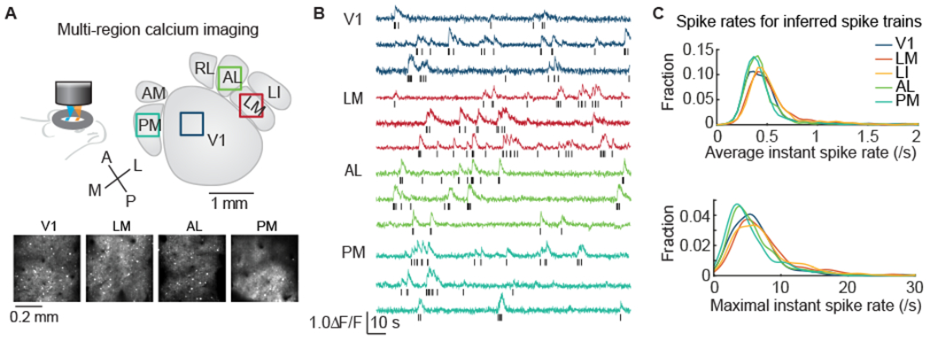
(A) Neuronal activity was imaged in multiple HVAs simultaneously using large field-of-view, temporally multiplexed, two-photon calcium imaging. In an example experiment, layer 2/3 excitatory neurons were imaged in V1, LM, AL, and PM simultaneously. Squares indicate the imaged regions, and projections of raw image stacks are shown below.

(B) Image stacks were analyzed to extract calcium dynamics from cell bodies, after neuropil subtraction. These traces were used to infer spike activity, as shown in raster plots below each trace.

(C) Statistics of inferred spiking were similar to those of prior reports, indicating accurate inference. The mean and maximal instantaneous firing rates of neurons in V1 and HVAs are similar (mean, 0.5 ± 0.5 spike/s; max, 7 ± 11 spike/s; p = 0.055 and p = 0.6).

We characterized the neuronal responses to three types of visual stimuli: scrolling textures (hereafter “texture stimuli”), random dot kinematograms (RDK), and a naturalistic video mimicking home cage navigation. Hundreds of neurons were recorded for V1, LM, AL and PM for all three stimuli, and LI were recorded for the texture stimuli (complete numbers are in Table S1). Neurons that exhibited reliable responses to a stimulus were included for further characterization (reliable neurons responded to > 50% of trials for RDK or texture stimuli; or exhibited trial-to-trial correlations > 0.08 with 0.5 s bins to naturalistic stimuli). These criteria resulted in 20 – 50% of all recorded neurons being included for further analysis (Table S1).

Texture and RDK stimuli were best represented in separate HVAs

We tested the selectivity of neurons in V1, LM, LI, AL and PM to texture stimuli using a set of naturalistic textures that drifted in one of the four cardinal directions (Figure S2A). We generated four families of texture images based on parametric models of naturalistic texture patterns³⁴. These stimuli allowed us to characterize the representation of both texture pattern information and drift direction information, and thus test the tolerance of a texture selective neuron to motion direction.

We observed reliable responses to drifting textures in V1, LM, LI, and PM. AL was less reliable in response to these stimuli (V1, LM, LI and PM have 33%~41% reliable neurons, while AL has 20% reliable neurons; p = 0.04 One-way ANOVA; Figure S2A and S2B). Texture informative neurons exhibited various selectivity patterns (Figure 2A). We measured neuronal selectivity to texture family, motions direction, or joint selectivity using mutual information analysis. Higher bit values for a neuron-stimulus parameter pair means that the activity from that neuron provides more information about that stimulus parameter (or combination of stimulus parameters). Overall, neurons in V1 and LI were more informative about the texture stimuli, followed by LM. By contrast, neurons in areas AL and PM were not informative about the texture stimuli (Figure 2B; p = 3.7 x 10⁻¹⁷; one-way ANOVA). To examine the tolerance of texture encoding neurons to the translational direction, we computed the mutual information between neuronal responses and texture families (refer to the statistical pattern of a texture image). LI was the most informative about texture family out of all tested visual areas, followed by V1 and LM (Figure S2C; p = 1.8 x 10⁻¹¹; one-way ANOVA). Meanwhile, V1, LM and LI also carried more information about the motion direction of the texture stimuli, compared to areas AL and PM (Figure S2D; p = 1.2 x 10⁻⁷, one-way ANOVA). Examining the information encoding of individual neurons, we found an increasing fraction of neurons that jointly encoded texture family and texture drift direction along the putative ventral pathway (V1: 7%, LM: 8%, LI: 14%, AL: 2%, PM: 1%; p = 9 x 10⁻¹²; one-way ANOVA; Figure 2C), suggesting increasing joint coding along the putative ventral visual hierarchy (V1 -> LM -> LI).

Figure 2. Segregated representations of textures and random dot kinematogram (RDK) motion in HVAs.

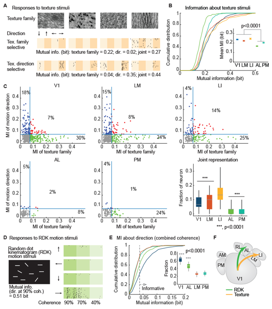
(A) Mice were shown texture stimuli, each of which was from one of four texture families, and drifted in one of four directions. Spike raster plots from two example neurons (10 trials shown for each) show that one neuron is selective for texture family, and the other is more selective for texture direction. The amount of mutual information (MI, in bits) for the two stimulus parameters (texture family and motion direction) are written below each raster, along with the overall or joint (family and direction) MI.

(B) V1, LM, and LI provide higher MI for texture stimuli than AL or PM (p = 3.7 x 10⁻¹⁷). Error bars in inset indicate SE.

(C) Relation between information about the moving direction and information about the texture family carried by individual neuron per visual area. Each dot indicates one neuron. Blue line indicates the threshold of significant amount of information, which was defined by shuffled data (Mean + 3*SD). Lower right: summarize the fraction of neurons exhibit significant joint representation (red dots). Distribution generated by permutation.

(D) Mice were shown random dot kinematogram (RDK) motion stimuli, which drifted in one of four directions with up to 90% coherence (fraction of dots moving in the same direction). A raster for an example neuron (30 trials) shows that it fires during rightward motion, with 0.51 bits of MI for motion direction at 90% coherence.

(E) Cumulative distribution plot of information about the motion direction combining all coherence levels. Gray dashed line indicates the threshold for a significant amount of information, which was defined by shuffled data (mean + 3*SD). (inset) A boxplot of the fraction of informative neurons generated by permutation.

(F) These results indicate a segregation of visual stimulus representations: texture stimuli to LM, and RDK motion stimuli to AL.

(B, C, E) p-values generated by one-way ANOVA with Bonferroni correction.

To further examine joint coding along the putative ventral hierarchy, we fit an encoder model to neurons that were significantly informative about the drift direction or the texture family (roughly half of the reliable neurons; Figure 2C). We decomposed the neuron model into the drifting direction component and the texture family component through SVD decomposition, and we quantified the number of drifting direction and the number of texture family one neuron was selective to in the SVD components (Figure S2E and S2F). Joint encoding neurons exhibited increasingly broader selectivity towards texture family and drifting directions along the putative ventral pathway (Figure S2G).

These results for texture encoding contrast with results for standard drifting gratings. For gratings, we found motion direction information to be encoded broadly, differing <10% among HVAs (Figure S2H), while texture motion information did not propagate to visual areas outside the putative ventral pathway, differing >200% among HVAs (Figure S2C and S2D). The drift speeds were similar (32 degrees/s for the textures and 40 degrees/s for the gratings), so it is unclear which spatial structural differences between these stimuli drove the differences in encoding. Thus, we next examined responses to a stimulus with less spatial structure and greater focus on motion.

We examined the encoding of random dot kinematograms (RDK), which are salient white dots on a dark background with 40-90% motion coherence (remaining dots move in random directions (Figure 2D). The RDK stimuli elicited reliable responses (responses to >50% trials) in neurons in V1, LM, AL and PM. For this stimulus, reliable neurons were common in V1 and rarer in LM (p = 0.001; one-way ANOVA; Figure S3A and S3B). To characterize the direction selectivity of reliable neurons, we computed the mutual information between neuronal responses and the motion direction at each coherence level. V1 and AL have larger fractions of informative neurons than LM and PM (p = 2.3 x 10⁻¹⁵, one-way ANOVA; Figure 2E). On average, V1 and AL were more informative than LM and PM about the motion direction of the RDK at moderate-to-high coherence levels (>=70%; Figure S3C and S3D; p = 3.3 x 10⁻¹⁰, one-way ANOVA). At low coherence level (40%), the differences among HVAs became insignificant (Figure S3D).

To further characterize the direction selectivity of neurons, we fit an encoder model to neurons that were significantly informative about the RDK stimuli. Followed by decomposing the neuron model into the direction component and the coherence component through SVD decomposition (Figure S3E, and S3F; Methods). We then identified the preferred direction and the preferred coherence level in these SVD components for individual neurons. Interestingly, the direction preference of V1 biased to a downward motion, or horizontal flows (p = 8.6 x 10⁻⁸, one-way ANOVA). However, in AL, an RDK representing HVA, such bias was not obvious (p = 0.09; one-way ANOVA; Figure S3G). All tested areas were modulated by coherence, and the highest coherence was preferred by the majority of neurons (Figure S3G).

In summary, texture selective neurons were more abundant in V1, LM, LI, while RDK direction selectivity neurons were more abundant in V1 and AL. Thus, information about drifting textures and RDK motion are relatively segregated to distinct HVAs (Figure 2F).

Features of naturalistic videos were best represented in separate HVAs

To determine whether this segregation of texture and motion information among HVAs could be detected within a more complex stimulus, we characterized the neuronal representation of a 64-second-long naturalistic video (Figure 3A). The naturalistic video stimulus contained time-varying visual features such as contrast^35,36, luminance, edge density³⁷, difference of Gaussian (DOG) entropy³⁸, and optic flow (OF) speed and direction³⁹ (Methods; Figure S4A–D). Both edge density and DOG entropy capture spatial properties of a naturalistic video frame, while DOG entropy better supports texture family encoding (Figure S4E and S4F). Our results thus far suggested that activity in AL would be modulated by motion information (OF speed or direction) in the naturalistic video, and activity in LM would be modulated by texture information (DOG entropy) in the same video.

Figure 3. Parametric features of the naturalistic video stimulus.

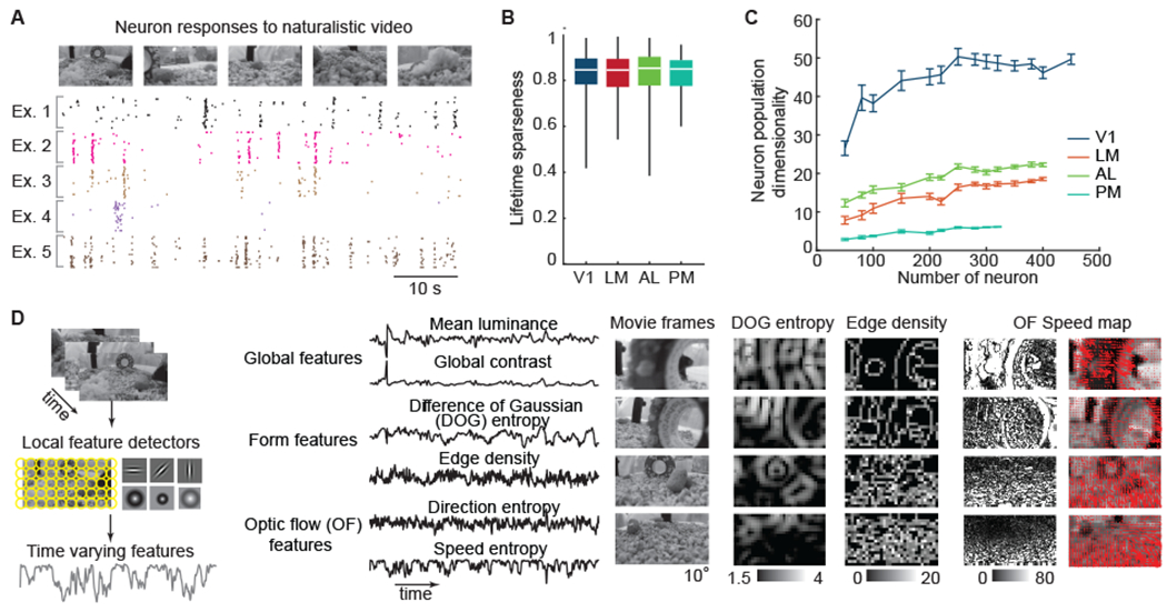
(A) Five example neurons show reliable, yet diverse, spike responses during a naturalistic video stimulus.

(B) Neurons in all four tested areas exhibited similarly high response sparseness to the naturalistic video (one-way ANOVA, p = 0.8).

(C) Dimensionality of neuron population responses versus the number of neurons per visual cortical area (error bars indicate SE of permutation).

(D) Form and motion components of the naturalistic video were extracted using a bank of linear filters with various sizes and locations (left). This provided time-varying signals correlated with global, form, and motion features, such as contrast, difference-of-Gaussian (DOG) entropy, and speed entropy (middle). To provide an intuitive feel for these features, example naturalistic video frames with the corresponding DOG entropy maps, edge density maps, and optical flow speed maps are shown (also see Figure S4A–C).

About 45% of V1 neurons and about 25% of LM, AL, and PM neurons responded to the naturalistic video reliably (trail-to-trial correlation > 0.08; Figure S5A). Neurons in the four imaged visual areas exhibited diverse and highly selective responses to the naturalistic video. Individual neurons responded to ~ 3% of stimulus video frames, corresponding to a high lifetime sparseness (0.83 ± 0.09 (mean ± SD); Figure 3B). The dimensionality of the population responses of V1 was about three-to-ten-times higher than those of LM, AL and PM (Figure 3C). The average response of a cortical area neuron population converged with several hundreds of neurons (about 500 from V1, about 200 from HVAs; Figure S5B). Thus, the data set has sufficiently covered the neuronal responses of V1, LM, AL, and PM to support further analysis. To take a data-driven approach to understanding the diverse response patterns, we classified neurons using an unbiased clustering method (Gaussian mixture model, GMM; Methods). Neurons were partitioned into 25 tuning classes based on their responses to the naturalistic video, and 21 of these classes exhibited unique sparse response patterns, responding at specific time points of the naturalistic video (Figure S5C and S5D). All tuning classes were observed in V1 and HVAs, but their relative abundance varied by area (Figure S5E and S5F). V1 had a relatively more uniform distribution of tuning classes compared to HVAs (Figure S5E). The lower dimensionality and biased distribution of tuning classes of HVAs can indicate selective representations of visual features.

To examine how well visual features (Figure S4D) of the naturalistic video were represented in HVAs, we computed the linear regression between responses of individual neurons, or population-averaged activity, with time-varying visual features of the naturalistic video (Fig. 3D). We defined the modulation power of each feature as the variance of responses explained by the model (i.e, the r² of a linear fit), and the modulation coefficients as the slope. The visual features were computed at multiple spatial scales (image filtered by Gaussian kernel with 1-25° full width at half maximum, FWHM), and qualitatively similar results were observed across a wide range of scales. Overall, the set of visual features explained 31% of the variance of the trial-averaged responses (with 0.5 s bins) of individual neurons across the visual areas. Representative results are obtained for edge density maps with a Gaussian kernel of 2.35° (FWHM), and DOG entropy maps with a Gaussian kernel of 11.75° (FWHM, inner kernel; the outer kernel is two-fold larger in FWHM) (Fig. 3D).

Regressing these visual features with individual neuronal responses revealed selective feature representations. AL neurons were more sensitive to the modulation by the OF speed entropy, while PM neurons were more sensitive to the modulation by contrast and edge density (Figure 4A). We further characterized the collective effects of biased distributions of tuning classes (from the GMM clustering analysis) among HVAs. Some tuning classes were more abundant in specific HVAs (relative to their abundance in V1), and we assessed their activity modulation by features in the naturalistic video. LM was enriched with neurons that correlated with DOG entropy (Figure 4B). As expected, AL and PM were enriched with tuning classes that correlate with the OF speed entropy feature, and the contrast and the edge density features, respectively (Figure 4B).

Figure 4. Segregated representations of spatial and motion features in naturalistic videos.

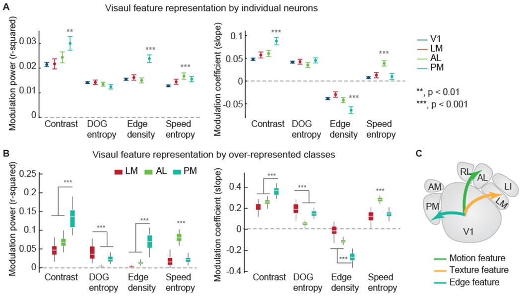
(A) The average modulation power (left) and the average modulation coefficients (right) of individual neuronal activity by visual features of the naturalistic video. The modulation power is characterized by the r-squared values (variance explained) of the linear regression.

(B) The time-varying features were weighted to best match the average neuronal activity of enriched classes for a cortical area (N = 200 with permutation; classes with red stars in Figure S5F). Areas LM was strongly modulated by DOG entropy. Area AL was strongly modulated by speed entropy. Area PM was modulated by contrast and edge density. The modulation coefficients were typically positive, but were negative for edge density. Thus, area PM is positively modulated by contrast, but negatively modulated by edge density. (p-values are from one-way ANOVAs with the Bonferroni correction for multiple comparison).

(C) These results indicate that visual feature components are segregated among HVAs: texture features to LM, motion features to AL, and fine edge features to PM.

Together, these results indicate that motion information and spatial information are differentially represented among HVAs due to the distribution of tuning classes among them. Neurons in AL provided superior representations of motion features in a naturalistic video, and neurons in LM and PM provided superior representations of texture and edge features, respectively, in the same naturalistic video (Figure 4C).

Gabor models exhibited biased feature representations

To this point, the evidence from the naturalistic stimuli indicates an enriched representation of spatial and motion features in LM, PM, and AL. We then questioned whether the feature enrichment in HVAs could be explained by receptive field (RF) structure. To model the receptive field structures of neurons, we employed a rich set of Gabor models, which are classic models for visual cortical neurons^40,41. Gabor models were simulated using a base model of a linear-nonlinear (LNL) cascade with Gabor filter-based linear kernels (Figure 5A). The set of models included 2D Gabor models with single or multiple sub-units combined linearly or quadratically (Figure 5B), as multiple Gabor kernels are required for predicting V1 neuron responses in mice⁴¹ and generating tolerances to rotation, translation, and scale^26,42. The set of models also included 3D Gabor kernels with or without untune normalization units (Figure 5B), as normalization is critical for capturing the diverse response profiles of V1 neurons to naturalistic stimuli⁴³. For 2D Gabor filter-based models, we examined both linear and energy models. These are similar to models of complex cells in which input from multiple simple cells with similar orientation preferences but varying phases are integrated¹². Other combinations were used as well (cross-orientation, cross-scale, etc.; Figure 5B). For 3D Gabor filter-based models, we also examined motion models (opponent motion energy²⁹; Figure 5B). The simulations were performed with multiple spatial scales and, for 3D Gabor filter-based models, temporal scales and sampled uniformly in space.

Figure 5. Spatial and motion feature encoding by variants of Gabor filter-based models.

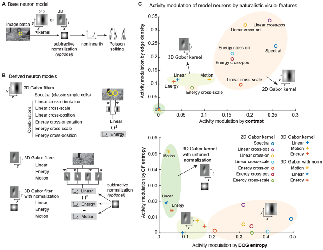
(A) The general architecture is a linear-nonlinear-Poisson (LNP) cascade neuron model. Neurons were simulated by various 2D and 3D Gabor-like linear kernels, with or without an untuned subtractive normalization.

(B) From the base LNP model, variations were derived, organized into three classes: 2D Gabor-based, 3D Gabor-based without normalization, and 3D Gabor-based with normalization. Both linear and energy responses (akin to simple cells and complex cells) were computed from combinations of 2D Gabor filters. Linear, energy and motion responses (akin to simple cells, complex cells, and speed cells) were computed from 3D Gabor filters.

(C) These three classes of models varied in how much their activity was modulated by global, form, and motion features in naturalistic videos. The neuron models are plotted by their modulation in feature spaces. The location of a neuron model was defined by the modulation power (same as Figure 4).

We determined the feature extraction properties of the models by simulating responses to the texture and RDK stimuli and characterizing them (Figure S6). Neuron models varied in the encoding power of different types of stimuli or visual features. We noted that 2D Gabor models exhibited specific tuning to the texture family while remaining tolerant to motion directions, especially the cross-orientation and linear cross-position models (Figure S6A), which are the best models for texture family encoding. On the other hand, 3D Gabor models with normalization performed the best in encoding the motion direction in RDK stimuli (Figure S6B).

In response to the naturalistic videos, 2D Gabor models, especially linear cross-position and linear cross-orientation models, exhibited better sensitivity to the contrast, edge density, and the DOG entropy, while the 3D Gabor models with untuned normalization exhibited better sensitivity to the OF entropy (Figure 5C). These simulation results confirmed the apparent trade-off in representation fidelity for spatial features and motion features, with 2D Gabor kernels performing better on the former, and 3D Gabor kernels with or without normalization, on the latter.

Gabor models reproduced specific feature representations of mouse visual cortex

Next, we determined the best Gabor model for neurons recorded in vivo to the naturalistic video stimuli. We fit individual neuronal responses with the Gabor-based models. One best model among the whole set, the “preferred” model, was selected for individual neurons. Preferred models captured the greatest amount of PSTH variance of the in vivo neuronal responses (Figure 6A). In general, the preferred models explained 40 ± 17 % (mean ± SD) of the variance of the PSTH (no difference between visual areas, one-way ANOVA p = 0.06).

Figure 6. HVA-specific enrichment of Gabor model types.

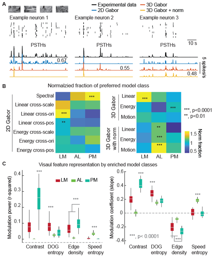
(A) Data from example neurons are shown in raster plots (top) and PSTHs (bottom), along with the best fits (as PSTHs) from each of the three model classes: 2D Gabor, 3D Gabor, and 3D Gabor with normalization. The numbers near the model PSTHs indicate the variance explained by the best models for that example neuron. One best model was selected for each neuron for the analysis in the following panels.

(B) For each Gabor model type and HVA, we computed how often that model was preferred for that HVA. Then, for each HVA, we normalized the model type fractions by the frequency for model types in V1.

(C) The modulation power (left) and the modulation coefficients (right) of the average responses of enriched model classes for HVAs (N = 50 with permutation; classes with stars in B).

(B, C) p-values from one-way ANOVAs to test the statistical difference among the three HVA areas.

V1 and HVAs varied in model preference. All classes were present in V1, but HVAs varied in the classes that were more or less frequently observed (Figure 6B). We found that LM was enriched with texture feature encoding models, such as 2D models with linear cross-orientation subunits, and linear cross-position subunits (Figure 6B). AL was enriched with, motion encoding models, such as 3D motion models with normalization (Figure 6B). In contrast, PM had an abundance of single-unit 2D models (spectral filters), which were sensitive to the contrast visual features (Figure 6B).

Using the preferred models that were enriched in each HVA, we reproduced the linear regression results between the features of the naturalistic video (Figure 3D) and the HVA-specific model responses (Figure 6C). In general, the model selection reflected the segregated representation of spatial and motion features by LM, AL, and PM. Overall, the Gabor model analysis revealed that LM, AL, and PM were enriched with different RF structures. LM had more 2D linear cross-orientation and linear cross-position RFs, as well as 3D simple cells. AL had more 3D simple, complex, and motion cells, and received surround normalization input. PM had more 2D simple cells and 3D complex cells. These insights into the RF structure of neurons in HVAs provide clues into potential neural circuitry underlying the varying representations of features in naturalistic stimuli.

Discussion

The results revealed unique encoding properties of L2/3 neurons of V1 and multiple HVAs in representing textures, motion, and naturalistic videos. Our results show that neurons in LM provide high fidelity representations of spatial features such as DOG entropy and textures, but are poor at representing motion. By contrast, neurons in AL provide high fidelity representations of motion features, but are poor at representing spatial features. Neurons in PM provide high fidelity representations of some spatial features like edge density and contrast, but not DOG entropy or textures as areas LM do. Relatedly, LM, LI, and AL are all poor at representing edge density. These findings show that visual features are represented in segregated neuronal populations, implying trade-offs in encoding. To investigate potential trade-offs, we examined receptive field structures of neurons in HVAs that contributed to specialized feature representations. Indeed, we found that different receptive field models were required for reproducing the in vivo results in separate HVAs. These findings provide new insights into the neural circuitry that can generate distributed representations of visual stimuli in HVAs.

The rodent visual system evolved in response to the ecological niche mice found themselves in. We do not expect such a process to result in neural circuitry that performs neat, absolute segregations of information about visual scenes. Instead, we expect neural circuitry that supports adaptive behavior for the mouse’s ecological niche, such as visual mechanism for predator avoidance^44,45. The principles of that circuitry are likely quite different from those of any systematic, mathematically compact approach for parsing a visual scene in terms of known receptive field properties of visual cortical neurons. Thus, here we used a data-driven approach to gain a conservative foothold into complex visual scene processing in mice. We explored how segregated representations might emerge using a modeling approach based on known receptive field properties of visual cortical neurons, or at least popular models thereof. This analysis showed that linear combination of edges and motion energy model with normalization provided accurate accounts for distinguishing texture and motion stimuli.

The enrichment of specific representations of motion or texture in L2/3 of areas AL and LM respectively, could arise from specific connectivity from other brain regions (e.g., V1) that preserves selectivity that arose there⁵, or from converging input that results in enhanced selectivity (i.e., more invariant selectivity) for a visual feature^12,41,46. We generally cannot distinguish those two possibilities with this data set. Dense feedback and feedforward connectivity between HVAs and V1 make it difficult to pinpoint where selectivity arises. However, area LI exhibited more complex selectivity than V1, so it appears as though preserved selectivity from V1 projecting to LI would be insufficient to produce such selectivity. Even then, we cannot rule out thresholding effects which could play a role in increasing apparent selectivity.

The dual-stream framework describes two subnetworks of visual circuitry, a ventral one for object recognition, and a dorsal one for motion and action^27,47. In primates, the ventral stream— from V1, through V2, V3, and V4, to the inferior temporal lobe— develops selective activity for specific recognized objects, including faces. The dorsal stream— from V1, through V2, MT, MST and the parietal lobe— processes the spatial and motion information in visual scenes. Anatomically, cat and ferret have similar visual hierarchies as primates. Cat areas 17, 18 and 19 are analogous to the V1, V2, and V3 of primates; and area 21a and posterior medial lateral suprasylvian sulcus (PMLS) are analogous to primates’ V4 and MT respectively^48–53. Robust representations of oriented gratings or edges are commonly found in V1, but how do representations change along the dorsal and ventral streams? Neurons in areas V2 and V4 can encode a combination of local features, such as multiple edges to detect curves and shapes^37,42. Neurons in areas MT and MST can encode opponent motion energy^29,54–56. However, conflicts and complexities have been identified for these apparently stream-segregated feature representations in primates^57,58. Cats and ferrets may have cortical circuitry that is functionally analogous to V4 and MT in primates^48,53,59, nevertheless our knowledge of intermediate-level feature representations in these animals is limited. Anatomical connectivity with downstream brain regions supports functional distinctions in mouse HVAs, between putative ventral and dorsal streams. For example, putative ventral areas are strongly connected to temporal and parahippocampal cortices, while putative dorsal areas are preferentially connected to parietal, motor and limbic areas³. However, there are also major differences. The cortical visual system of mice is distinct from primates, cats, and ferrets, which have a single V2 adjacent to V1⁶⁰. Instead, mice have more than seven HVAs that share a border with V1^8,60. These anatomical differences complicate the search for the dual stream homologies in mice, and motivate functional studies to elucidate the information processing in mouse HVAs²⁷. The functional similarities between mouse LM and LI and macaque V2 and V4, and between mouse AL and macaque MT are perhaps superficial, but could also indicate that the dual stream framework for visual pathways in primates could have an analog in mice^3,61. Anatomical and receptive field mapping studies suggest that mouse LM and AL likely serve as the ventral and dorsal gateways in the mouse visual hierarchy^4,8,62.

Our experimental results reveal segregations of visual encoding, or representations, among HVAs in mice. The modeling results demonstrate how classic models of visual cortex neuron receptive fields can entail reciprocal trade-offs for representing spatial features and motion features of visual stimuli, thus providing a potential functional substrate for this segregation. These insights show how mouse HVAs likely play distinct roles in visual behaviors, and may share similarities with the dual processing streams in primates.

STAR Methods

RESOURCE AVAILABILITY

Lead contact

Requests for additional information or resources related to the study should be directed to Spencer L. Smith (sls@ucsb.edu).

Materials availability

This study did not generate new unique reagents.

Data and code availability

• Deconvolved spike data, and key functions for Gabor modeling and naturalistic video processing are available in: https://github.com/yuyiyi/HVA_tuning.git

• Code for calcium imaging processing is available in: https://github.com/yuyiyi/CaSoma_Proc.git

• Any additional information required to reanalyze the data reported in this paper is available from the lead contact upon request.

EXPERIMENTAL MODEL AND SUBJECT DETAILS

Subjects

All animal procedures and experiments were approved by the Institutional Animal Care and Use Committee of the University of North Carolina at Chapel Hill or the University of California Santa Barbara and performed in accordance with the regulation of the US Department of Health and Human Services. Total of 34 GCaMP6s-expressing transgenic adult mice of both sexes were used in this study. Mice were 110 – 300 days old for data collection. GCaMP6s-expressing mice were induced by triple crossing of the following mouse lines: TITL-GCaMP6s (Allen Institute Ai94), Emx1-Cre (Jackson Labs #005628), and ROSA:LNL:tTA (Jackson Labs #011008)³¹. Mice were housed under a 12 h light / 12 h dark cycle, and experiments were performed during the dark cycle of mice.

METHOD DETAILS

Surgery

For cranial window implantation, mice were anesthetized with isoflurane (1.5 – 1.8% in oxygen) and acepromazine (1.5 – 1.8 mg/kg body weight). Carprofen (5 mg/kg body weight) was administered prior to surgery. Body temperature was maintained using physically activated heat packs or homeothermic heat pads during surgery. Eyes were kept moist with ophthalmic ointment during surgery. The scalp overlaying the right visual cortex was removed, and a custom steel headplate with a 5 mm diameter opening was mounted to the skull with cyanoacrylate glue (Oasis Medical) and dental acrylic (Lang Dental). A 4 mm diameter craniotomy was performed over the visual cortex and covered with a #1 thickness coverslip, which was secured with cyanoacrylate glue.

Intrinsic signal optical imaging (ISOI)

Prior to two-photon imaging, the locations of primary and higher visual areas were mapped using ISOI, as previously reported^4,30,63. Pial vasculature images and intrinsic signal images were collected using a CCD camera (Teledyne DALSA 1M30) and a tandem lens macroscope. A 4.7 × 4.7 mm² cortical area was imaged at 9.2 μm/pixel spatial resolution and at 30 Hz frame rate. The pial vasculature was illuminated and captured through green filters (550 ± 50 nm and 560 ± 5 nm, Edmund Optics). The ISO images were collected after focusing 600 μm down into the brain from the pial surface. The intrinsic signals were illuminated and captured through red filters (700 ± 38 nm, Chroma and 700 ± 5 nm, Edmund Optics). Custom ISOI instrumentation was adapted from Kalatsky and Stryker⁹. Custom acquisition software for ISOI imaging collection was adapted from David Ferster³⁰. During ISOI, mice were 20 cm from a flat monitor (60 × 34 cm²), which covered the visual field (110° x 75°) of the left eye. Mice were lightly anesthetized with isoflurane (0.5%) and acepromazine (1.5 – 3 mg/kg). The body temperature was maintained at 37 °C using a custom electric heat pad³⁰. Intrinsic signal responses to vertical and horizontal drifting bars were used to generate retinotopic maps for azimuth and elevation. The retinotopic maps were then used to locate V1 and HVAs (Figure S1A). Borders between these areas were drawn using features of the elevation and azimuth retinotopic maps, such as reversals, manually^4,16. The vasculature map provided landmarks to identify visual areas in two-photon imaging.

In vivo two-photon imaging

Two-photon imaging was performed using a custom Trepan2p microscope controlled by custom LabView software³⁰. Two regions were imaged simultaneously using temporal multiplexing³⁰. Two-photon excitation light from an ultrafast Ti:Sapph laser tuned to 910 nm (MaiTai DeepSee; Newport Spectra-Physics) laser was split into two beams through polarization optics, and one path was delayed 6.25 ns relative to the other. The two beams were steered independently from each other using custom voice coil steering mirrors and tunable lenses. This way, the X, Y, Z plane of the two paths can be independently positioned anywhere in the full field (4.4 mm diameter). The two beams were raster scanned synchronously about their independently positioned centers by a 4 kHz resonant scanner and a linear scanner (Cambridge Technologies). Photons were detected (H7422P-40, Hamamatsu) and demultiplexed using fast electronics. For four-region scanning, the steering of the two beams was alternated every other frame.

In the current study, two-photon imaging of 500 x 500 μm² was collected at 13.3 Hz for two-region imaging, or 6.67 Hz for large-field single path imaging (Table S1). We typically imaged neurons in V1 and one or more HVAs simultaneously. Up to 500 neurons (V1: 129 ± 92; HVAs: 94 ± 72; mean ± SD) were recorded per imaging region (500 x 500 μm²). Imaging was performed with typically <80 mW of 910 nm excitation lights out of the front of the objective (0.45 NA), including both multiplexed beams together. Mice were head-fixed about 11 cm from a flat monitor, with their left eye facing the monitor, during imaging. The stimulus display monitor covered 70° x 45° the left visual field. Two-photon images were recorded from awake mice. During two-photon imaging, we monitored the pupil position and diameter using a custom-controlled CMOS camera (GigE, Omron) at 20 – 25 fps. No additional illumination was used for pupil imaging.

Visual stimuli

Visual stimuli were displayed on a 60 Hz LCD monitor (9.2 x 15 cm²). All stimuli were displayed in full contrast.

The texture stimuli (Figure S2A) were generated by panning a window over a large synthesized naturalistic texture image at one of the cardinal directions at the speed of 32 °/s. We generated the large texture image by matching the statistics of naturally occurring texture patterns³⁴. The texture pattern families were: animal fur, mouse chow, rocks, and tree trunk. Each texture stimulus ran for 4 s and was interleaved by a 4 s gray screen.

The random dot kinematogram (RDK) stimuli contained a percentage (i.e., coherence) of white dots that move in the same direction (i.e., global motion direction) on a black background (Figure S3A). We presented the animal with RDK at three coherence levels (40%, 70%, and 90%) and four cardinal directions. The dot diameter was 3.8° and the dot speed was 48 °/s. White dots covered about 12.5% of the screen. The lifetime of individual dots were about 10 frames (1/6 s). These parameters were selected based on mouse behavior in a psychometric RDK task⁶⁴. Each RDK stimulus ran for 3 – 7 s (responses in the first 3 s were used for analysis) and interleaved with 3 s gray screen. The same RDK pattern was looped over trials.

Two naturalistic videos (Figure 3A) were taken by navigating a mouse home cage, with or without a mouse in the cage. Each video had a duration of 32 s and were presented with interleaved 8 s long periods with a gray screen. For the convenience of analysis, we concatenated the responses to the two videos (total 64 s).

QUANTIFICATION AND STATISTICAL ANALYSIS

Calcium imaging processing

Calcium imaging processing was carried out using custom MATLAB codes. Two-photon calcium imaging was motion corrected using Suite2p subpixel registration module⁶⁵. Neuron ROIs and cellular calcium traces were extracted from imaging stacks using custom code adapted from Suit2p modules⁶⁵ (https://github.com/cortex-lab/Suite2P). Neuropil contamination was corrected by subtracting the common time series (1^st principal component) of a spherical surrounding mask of each neuron from the cellular calcium traces^15,66.

Neuropil contamination corrected calcium traces were then deconvolved using a Markov chain Monte Carlo (MCMC) methods⁶⁷ (https://github.com/flatironinstitute/CalmAn-MATLAB/tree/master/deconvolution; Figure S1B). For each calcium trace, we repeated the MCMC simulation for 400 times, and measured the reproducibility of MCMC spike train inference for each cell. We computed the Pearson correlation of the entire inferred spike train (tens of mins duration) binned at 13.3 fps. For all subsequent analysis, only cells with stable spike train inference results were included (correlations between MCMC simulations > 0.2). The number of neurons passed this criterion was defined as the total number of neurons (Table S1). The MCMC quality control was defined empirically. For all following analysis, we randomly pick one simulation trial for each neuron. Randomly picking a different trial did not affect results quantitatively.

Neurons in V1 and HVAs exhibited similar instantaneous firing rates, defined as inverse of inter-spike-interval (Figure 1C). Maximal instantaneous firing rates were computed as the inverse of the minimal inter-spike-interval, while average instantaneous firing rates were computed as the inverse of the average inter-spike-interval for individual neurons.

Reproducibility and lifetime sparseness

The reproducibility of responses to naturalistic videos was defined as the trial-to-trial Pearson correlation between inferred spike trains of each neuron binned in 500 ms bins. The reproducibility of responses to texture stimuli and RDK were computed as the fraction of trials that a neuron fired to its preferred stimulus within a time window (4 s for texture stimuli and 3 s for RDK). These definitions were commonly used in previous studies^46,68. Only reliably responsive neurons were included in the latter analysis (Pearson correlation > 0.08 to naturalistic video; fired on > 50% trials to the texture and RDK stimuli). The qualitative results were not acutely sensitive to the selection criteria.

The lifetime sparseness defines how often one neuron response to a particular stimulus was computed as (eq. 1)⁶⁹:

$$S=\frac{1-\frac{1}{N}\ast \frac{{({\sum }_i{r}_i)}^2}{{\sum }_i{r}_i^2}}{1-\frac{1}{N}}$$ (eq. 1)

For lifetime sparseness, r_i is trial-averaged response to i^th stimulus and N is the length of the stimuli. The sparseness to naturalistic videos was computed using 500 ms bins. The qualitative results of reliability and sparseness were not acutely sensitive to the bin size.

Information analysis

Mutual information (MI) evaluates the information the neuronal response (r) has about certain aspects of the stimulus, and it is computed in units of bits. It was computed using the following equation.

$$MI(r,s)=\sum _r\sum _s{p}_{r,s}(r,s)\ast {\log }_2\frac{p_{r,s}(r,s)}{p_r(r)\ast p_s(s)}$$ (eq. 2)

We computed the MI between neuron responses and the visual stimulus (s has 16 categories for texture stimuli, p_s(s) = 1/16; s has 12 categories for RDK, p_s(s) = 1/12). We also computed the MI between neuron responses and the texture family (s has 4 categories for texture stimuli, p_s(s) = 1/4), and the MI between neuron responses and the moving directions (s has 4 categories for both texture stimuli and RDK, p_s(s) = 1/4). The probability of neuron responses was computed from spike count distributions within a stimulus window (4 s for texture stimulus and 3 s for RDK). Reliable RDK and texture reliable neurons (response to >50% of trials) were included for the MI analysis.

Informative neurons:

We defined threshold for informative neurons from shuffled data (> mean + 3 SD of MI of shuffled data). That is the spike count (p_r,s(r, s)) of a neuron shuffled on each trial independently.

Tuning pattern of informative neurons

To estimate the tuning pattern of informative neurons, i.e., which texture pattern or motion direction one neuron responded to, or how many texture patterns one neuron responded to, we decomposed the neuronal responses into motion direction components, and texture family or RDK coherence components using singular value decomposition (SVD). To be more robust, instead of using trial-averaged response, we first estimated the neuronal responses by linearly regressing with a unit encoding space (Figure S2E and S3E). Lasso regularization was applied to minimize overfitting. The regularization hyper-parameters were selected by minimizing the cross-validation error in predicting single trial neuronal responses. The linear regression model performance was measured by the Pearson correlation between the trial-averaged neuron response and the model. All informative neurons were well-fit by the model (Figure S2F and S3F).

We then characterized the SVD components of all informative neurons. The SVD vectors reflect the selectivity of a neuron. Absolute values close to one indicate a preferred stimulus while values close to zeros indicate a null stimulus. Some texture informative neurons were activated by multiple texture patterns or motion directions, which were identified as the components that have a >0.4 absolute SVD vector value (qualitative results hold with similar thresholds). We quantified the number of texture patterns and the number of motion directions one texture informative neuron was responsive to (Figure S2G). Also, we identified the preferred motion direction and coherence level for RDK informative neurons (Figure S3G).

Population response dimensionality

We measured the dimensionality of neuron populations with certain size through principal components analysis of trial-averaged response of neurons (spike trains were binned in 500 ms). We generated principal components of each population by the trial-averaged responses that were computed using randomly selected half of the trials (training data), and then used the first x number of principal components to recover the trial-averaged responses of the remaining half of the trials (testing data). The dimensionality was defined as the number of principal components that reproduced the testing data that minimize the mean squared error.

Gaussian mixture model

To characterize the tuning properties in an unbiased manner, neurons were clustered using a Gaussian mixture model⁷⁰ (GMM) based on the trial-averaged responses to the naturalistic video. Only reliably responsive neurons were included for GMM analysis (trial-to-trial Pearson correlation of the inferred spike trains > 0.08, after spike trains were binned in 500 ms bins). Neuronal responses of the whole population, pooled overall cortical areas, were first denoised and reduced in dimension by minimizing the prediction error of the trial-averaged response using principal component (PC) analysis. 45 PCs were kept for population responses to the naturalistic videos. We also tested a wide range of PCs (20 – 70) to see how this parameter affected clustering, and we found that the tuning group clustering was not acutely affected by the number of PCs used. Neurons collected from different visual areas and different animals were pooled together in training the GMM (3839 neurons). GMMs were trained using the MATLAB build function fitgmdist with a range of numbers of clusters. A model of 25 classes was selected based on the Bayesian information criterion (BIC). We also examined models with different numbers of classes (20, 30, 45, or 75), and found that the main results held regardless of the number of GMM classes. Neurons with similar response patterns were clustered into the same class. Figure S5C shows the response pattern of GMM classes to the naturalistic video. The size of the naturalistic video classes is shown in Figure S5D. To examine the reproducibility of the GMM classification, we performed GMM clustering on 10 random subsets of neurons (90% of all neurons). We found the center of the Gaussian profile of each class was consistent (Pearson correlation of class centers, 0. 74 +/− 0.12). About 65% of all neurons were correctly (based on the full data set) classified, while 72% of neurons in classes that are over-represented in HVAs were correctly classified. Among misclassifications, about 78% were due to confusion between the three untuned classes with tuned classes. Thus, most of the classes to come out of the GMM analysis appear to be reproducible, and are not sensitive to specific subsets of the data.

Visual features of the naturalistic video

We characterized various visual features of the naturalistic video (Supplementary Fig. 5).

Average luminance:

The average pixel value of each frame.

Global contrast:

The ratio between the standard deviation of pixel values in a frame, and the average luminance of that same frame.

Edge density:

The local edges were detected by a Canny edge detector⁷¹. The algorithm finds edges by the local intensity gradient and guarantees to keep the maximum edge in a neighborhood while suppressing non-maximum edges. We applied the Canny edge detector after Gaussian blurring of the original image at multiple scales (1°-10°). A binary edge map was generated as the result of edge detection (Figure S4A). The edge density was computed as the sum of positive pixels in the binary edge map of each frame.

Difference of Gaussian (DOG) entropy:

We characterized local luminance features following the difference of Gaussian filtering at multiple scales, and then computed the entropy of these features within a local neighborhood (Figure S4B).

Optical flow entropy:

We estimated the direction and speed of salient features (e.g., moving objects) using the Horn-Schunck method at multiple spatial scales. Then we computed the entropy of the OF direction and speed at each frame. Since the OF estimation relies on the saliency of visual features, the moving texture and RDK stimuli resulted in distinct OF entropies, with the latter being larger (Figure S5C).

Visual features were computed either by average over space or by computing a spatial variance value (i.e., entropy). These measurements were inspired by the efficient coding theory⁷², which suggested that the neuron population coding is related to the abundance or the variance of visual features in the natural environment.

Discrimination of texture images by DOG features:

We computed the pairwise distance between texture images (Figure S4E) within the same class or from different classes (Figure S4F). The Euclidean distance was computed using DOG entropy (11.75° spatial filter size) or edge density (2.35° spatial filter size) feature maps. We then trained a support vector machine (SVM) classifier to discriminate texture images within and across classes, based on this pairwise distance (using the Matlab built-in function classify). We reported the cross-validation classification error rate (Figure S4F).

Modulation power of naturalistic features

A linear regression model was fit to the neuronal activity of individual neurons or average population response with individual features (Figure 4). These features are described above in the section (Visual features of the naturalistic video). We then evaluated a feature’s contribution in modulating the average population responses by the variance explained (r-squared) of each model (Figure 3D). Features were computed over multiple spatial scales. The spatial scales that best modulated (highest r-squared) the neuronal response was used for this analysis.

Neuronal activity of individual neurons or population average response were binning into 50 ms bins (50 – 500 ms bins were tested and generated qualitatively similar results). To evaluate the functional contribution of over-represented classes of HVAs, we pooled neurons from over-represented tuning classes of one HVA (200 neurons per pool with permutation; 50 – 200 pool size was tested and results hold), and we averaged activity over the pool, and then determined which features modulated activity the over-represented classes in an HVA (Figure 4B).

Gabor-based receptive field models

The neuron models used the structure of a linear-nonlinear (LNL) cascade. The spiking of model neurons was simulated following a nonhomogeneous Poisson process with a time varying Poisson rate. The rate was calculated by convolving visual stimuli with a linear kernel or a combination of linear kernels, followed by an exponential nonlinearity (Figure 5A). Linear kernels were modeled by 2D (XY spatial) or 3D Gabor (XYT spatiotemporal) filters defined over a wide range of spatiotemporal frequencies and orientations. We simulated neurons with simple cells, complex cells and motion cells models²⁹ (Figure 5B). The three differed in the linear components of the LNL cascade: simple cells (called linear model, or spectral model for the 2D Gabor kernels) used the linear response of a Gabor filter; complex cells (called energy model) used the sum of the squared responses from a quadrature pair of Gabor filters (90° phase shifted Gabor filter pairs); speed cells (called motion model) used the arithmetic difference between the energy responses from an opponent pair of complex cells. We also modeled neurons based on the cross product of the linear or energy responses from two 2D Gabor filters. In particular, we simulated the following three combination models: 1. 2D Gabor filters matched in spatial scale and location but tuned to different orientations (cross-orientation model); 2. 2D Gabor filters tuned to the same orientation and location with different spatial scales (cross-scale model); 3. 2D Gabor filters with matched tuning properties but offset in visual space (cross-position model) (Figure 5B). In addition, we included a subtractive normalization before taking the nonlinearity in some models. A total of 13 Gabor model types were used (Figure 5B).

To examine feature encoding by these neuron model types, we performed 10 – 20 repeats of simulation for each neuron model to each stimulus. Either the simulated spike trains or peristimulus time histograms (PSTH) were used for characterizing the feature encoding. We analyzed the model responses in the same way as we had done for the mouse experimental data. We computed the mutual information between simulated neuron responses and texture stimuli or RDK stimuli, and characterized the selectivity of simulated neurons to texture families or RDK directions (Figure S6). Next, we examined the modulation of simulated population responses by visual features of the naturalistic video. Neuron models were located in the feature space by how much of the population response variance was explained by individual features (Figure 5C).

Fit neuron responses with Gabor-based models

We fit individual neuronal responses with models following a linear regression equation (eq. 3). The linear coefficients were optimized by minimizing the cross-validation error. We also tested a sigmoidal nonlinear fitting (eq. 4). Sigmoidal parameters were optimized through gradient descent. As sigmoidal nonlinearity did not significantly improve the modeling performance, we reported the results from the linear fitting.

$$neuronresponse=a\ast x;$$ (eq. 3)

$$neuronresponse=\frac{a}{1+\exp (-b\ast x+c)};$$ (eq. 4)

Where x is the simulated response and a – c are parameters for fitting. Neuron models were grouped into three categories: 2D Gabor models, 3D Gabor models, and 3D Gabor models with normalization. One model of each category, which minimizes the cross-validation error, was kept for each neuron. Then, we selected the one among the three that maximize the variance explained of the PSTH for each neuron (Figure 6A). HVAs varied in their preference of different model types (Figure 6B). We then examined the modulation power of naturalistic visual features of enriched neuron models.

Statistical analysis and data availability

P-values were generated by one-way ANOVA with Bonferroni multiple comparison if not otherwise stated. Detailed statistical values were provided in the figure legends. Boxplot whiskers indicate the full data range.

KEY RESOURCES TABLE

REAGENT or RESOURCE	SOURCE	IDENTIFIER
Experimental Models: Organisms/Strains
Mouse: Emx1-cre; Ai94D (TITL-GCamp6s); ROSA-tTA	The Jackson Laboratory	Strain: jax #005628, Jax #024104, Jax # 011008
Software and Algorithms
MATLAB R2015b, 2019b	Mathworks	https://www.mathworks.com/products/matlab.html
suite2p calcium imaging processing toolbox	Pachitariu et al.65	https://github.com/cortex-lab/Suite2P
MCMC spike deconvolution toolbox	Pnevmatikakis et al.67	https://github.com/flatironinstitute/CaImAn-MATLAB/tree/master/deconvolution
Gabor modeling and naturalistic video processing	This paper	https://github.com/yuyiyi/HVA_tuning.git

Highlights.

• Texture stimuli are best represented in areas LM & LI, compared to areas AL & PM.

• Motion stimuli are best represented in area AL compared to areas LM & PM.

• Texture and motion components of naturalistic videos are similarly segregated.

• Receptive field models show trade-off for representations of motion versus texture.

References

- 1.Siegle JH, Jia X, Durand S, Gale S, Bennett C, Graddis N, Heller G, Ramirez TK, Choi H, Luviano JA, et al. (2021). Survey of spiking in the mouse visual system reveals functional hierarchy. Nature, 11–16. [DOI] [PMC free article] [PubMed] [Google Scholar]
- 2.Miyamichi K, Amat F, Moussavi F, Wang C, Wickersham I, Wall NR, Taniguchi H, Tasic B, Huang ZJ, He Z, et al. (2011). Cortical representations of olfactory input by trans-synaptic tracing. Nature 472, 191–6. [DOI] [PMC free article] [PubMed] [Google Scholar]
- 3.Wang Q, Sporns O, and Burkhalter A (2012). Network Analysis of Corticocortical Connections Reveals Ventral and Dorsal Processing Streams in Mouse Visual Cortex. J. Neurosci 32, 4386–4399. [DOI] [PMC free article] [PubMed] [Google Scholar]
- 4.Smith IT, Townsend LB, Huh R, Zhu H, and Smith SL (2017). Stream-dependent development of higher visual cortical areas. Nat. Neurosci 20, 200–208. [DOI] [PMC free article] [PubMed] [Google Scholar]
- 5.Glickfeld LL, Andermann ML, Bonin V, and Reid RC (2013). Cortico-cortical projections in mouse visual cortex are functionally target specific. Nat. Neurosci 16, 219–26. [DOI] [PMC free article] [PubMed] [Google Scholar]
- 6.Kim M, Znamenskiy P, Iacaruso MF, and Mrsic-flogel TD (2018). Segregated Subnetworks of Intracortical Projection Neurons in Primary Visual Cortex Highlights. Neuron, 1–9. [DOI] [PubMed] [Google Scholar]
- 7.Garrett ME, Nauhaus I, Marshel JH, and Callaway EM (2014). Topography and Areal Organization of Mouse Visual Cortex. J. Neurosci 34, 12587–12600. [DOI] [PMC free article] [PubMed] [Google Scholar]
- 8.Wang Q, and Burkhalter A (2007). Area Map of Mouse Visual Cortex. J. Comp. Neurol 502, 339–357. [DOI] [PubMed] [Google Scholar]
- 9.Kalatsky VA, Stryker MP, and Foundation WMK (2003). New paradigm for optical imaging: Temporally encoded maps of intrinsic signal. Neuron 38, 529–545. [DOI] [PubMed] [Google Scholar]
- 10.Schuett S, Bonhoeffer T, and Hübener M (2002). Mapping retinotopic structure in mouse visual cortex with optical imaging. J. Neurosci 22, 6549–6559. [DOI] [PMC free article] [PubMed] [Google Scholar]
- 11.Yu Y, Stirman JN, Dorsett CR, and Smith SL (2018). Mesoscale correlation structure with single cell resolution during visual coding. bioRxiv, 469114. [Google Scholar]
- 12.Hubel DH, and Wiesel T (1962). AND FUNCTIONAL ARCHITECTURE IN THE CAT ’S VISUAL CORTEX From the Neurophysiolojy Laboratory , Department of Pharmacology central nervous system is the great diversity of its cell types and inter- receptive fields of a more complex type (Part I) and to. J. Physiol 160, 106–154. [DOI] [PMC free article] [PubMed] [Google Scholar]
- 13.Jin M, and Glickfeld LL (2020). Mouse Higher Visual Areas Provide Both Distributed and Specialized Contributions to Visually Guided Behaviors. Curr. Biol 30, 4682–4692.e7. [DOI] [PMC free article] [PubMed] [Google Scholar]
- 14.Stringer C, Michaelos M, Tsyboulski D, Lindo SE, and Pachitariu M (2021). High-precision coding in visual cortex. Cell 184, 2767–2778.e15. [DOI] [PubMed] [Google Scholar]
- 15.Andermann ML, Kerlin AM, Roumis DK, Glickfeld LL, and Reid RC (2011). Functional Specialization of Mouse Higher Visual Cortical Areas. Neuron 72, 1025–1039. [DOI] [PMC free article] [PubMed] [Google Scholar]
- 16.Marshel JH, Garrett ME, Nauhaus I, and Callaway EM (2011). Functional specialization of seven mouse visual cortical areas. Neuron 72, 1040–1054. [DOI] [PMC free article] [PubMed] [Google Scholar]
- 17.Goltstein PM, Reinert S, Bonhoeffer T, and Hübener M (2021). Mouse visual cortex areas represent perceptual and semantic features of learned visual categories. Nat. Neurosci 24. [DOI] [PMC free article] [PubMed] [Google Scholar]
- 18.Tinsley CJ, Webb BS, Barraclough NE, Vincent CJ, Parker A, and Derrington AM (2003). The nature of V1 neural responses to 2D moving patterns depends on receptive-field structure in the marmoset monkey. J. Neurophysiol 90, 1263. [DOI] [PubMed] [Google Scholar]
- 19.Juavinett ALL, Callaway EMM, Information S, Juavinett ALL, and Callaway EMM (2015). Pattern and Component Motion Responses in Mouse Visual Cortical Areas. Curr. Biol 25, 1759–1764. [DOI] [PMC free article] [PubMed] [Google Scholar]
- 20.Zoccolan D (2015). Invariant visual object recognition and shape processing in rats. Behav. Brain Res 285, 10–33. [DOI] [PMC free article] [PubMed] [Google Scholar]
- 21.Tafazoli S, Safaai H, De Franceschi G, Rosselli FB, Vanzella W, Riggi M, Buffolo F , Panzeri S, and Zoccolan D (2017). Emergence of transformation-tolerant representations of visual objects in rat lateral extrastriate cortex. Elife 6, 1–39. [DOI] [PMC free article] [PubMed] [Google Scholar]
- 22.Chang L, and Tsao DY (2017). The Code for Facial Identity in the Primate Brain. Cell 169, 1013–1028.e14. [DOI] [PMC free article] [PubMed] [Google Scholar]
- 23.Froudarakis E, Cohen U, Diamantaki M, Walker EY, Reimer J, Berens P, Sompolinsky H, and Tolias AS (2020). Object manifold geometry across the mouse cortical visual hierarchy. bioRxiv, 2020.08.20.258798. [Google Scholar]
- 24.Yu Y, Hira R, Stirman JN, Yu W, Smith IT, and Smith SL (2018). Mice use robust and common strategies to discriminate natural scenes. Sci. Rep 8, 1–36. [DOI] [PMC free article] [PubMed] [Google Scholar]
- 25.Victor JD, Conte MM, and Chubb CF (2017). Textures as Probes of Visual Processing. Annu. Rev. Vis. Sci 3, 275–296. [DOI] [PMC free article] [PubMed] [Google Scholar]
- 26.Freeman J, Ziemba CM, Heeger DJ, Simoncelli EP, and Movshon JA (2013). A functional and perceptual signature of the second visual area in primates. Nat. Neurosci 16, 974–981. [DOI] [PMC free article] [PubMed] [Google Scholar]
- 27.Cadieu CF, and Olshausen BA (2012). Learning intermediate-level representations of form and motion from natural movies. Neural Comput. 24, 827–866. [DOI] [PubMed] [Google Scholar]
- 28.Zehi S, and Shipp S (1988). The functional logic of cortical connections. Nature 335, 311–317. [DOI] [PubMed] [Google Scholar]
- 29.Adelson EH, and Bergen JR (1985). Spatiotemporal energy models for the perception of motion. J. Opt. Soc. Am. A 2, 284. [DOI] [PubMed] [Google Scholar]
- 30.Stirman Jeffrey N., Smith Ikuko T., Kudenov Michael W., S. SL. (2016). Wide field-of-view, multi-region two-photon imaging of neuronal activity. Nat. Biotechnol 34, 857–862. [DOI] [PMC free article] [PubMed] [Google Scholar]
- 31.Madisen L, Garner AR, Shimaoka D, Chuong AS, Klapoetke NC, Li L, van der Bourg A, Niino Y, Egolf L, Monetti C, et al. (2015). Transgenic Mice for Intersectional Targeting of Neural Sensors and Effectors with High Specificity and Performance. Neuron 85, 942–958. [DOI] [PMC free article] [PubMed] [Google Scholar]
- 32.Chen TW, Wardill TJ, Sun Y, Pulver SR, Renninger SL, Baohan A, Schreiter ER, Kerr RA, Orger MB, Jayaraman V, et al. (2013). Ultrasensitive fluorescent proteins for imaging neuronal activity. Nature 499, 295–300. [DOI] [PMC free article] [PubMed] [Google Scholar]
- 33.Niell CM, and Stryker MP (2008). Highly Selective Receptive Fields in Mouse Visual Cortex. J. Neurosci 28, 7520–7536. [DOI] [PMC free article] [PubMed] [Google Scholar]
- 34.Portilla J, and Simoncelli EP (2000). Parametric texture model based on joint statistics of complex wavelet coefficients. Int. J. Comput. Vis 40, 49–71. [Google Scholar]
- 35.Prusky GT, and Douglas RM (2004). Characterization of mouse cortical spatial vision. Vision Res. 44, 3411–3418. [DOI] [PubMed] [Google Scholar]
- 36.Goldbach HC, Akitake B, Leedy CE, and Histed MH (2021). Performance in even a simple perceptual task depends on mouse secondary visual areas. Elife 10, 1–39. [DOI] [PMC free article] [PubMed] [Google Scholar]
- 37.Ziemba CM, Freeman J, Movshon JA, and Simoncelli EP (2016). Selectivity and tolerance for visual texture in macaque V2. Proc. Natl. Acad. Sci 113, E3140–3149. [DOI] [PMC free article] [PubMed] [Google Scholar]
- 38.Duan H, and Wang X (2015). Visual attention model based on statistical properties of neuron responses. Sci. Rep 5, 8873. [DOI] [PMC free article] [PubMed] [Google Scholar]
- 39.Sit KK, and Goard MJ (2020). Distributed and retinotopically asymmetric processing of coherent motion in mouse visual cortex. Nat. Commun 11, 1–14. [DOI] [PMC free article] [PubMed] [Google Scholar]
- 40.Carandini M, Heeger DJ, and Movshon JA (1997). Linearity and Normalization in Simple Cells of the Macaque Primary Visual Cortex. J. Neurosci 17, 8621–8644. [DOI] [PMC free article] [PubMed] [Google Scholar]
- 41.Yoshida T, and Ohki K (2020). Natural images are reliably represented by sparse and variable populations of neurons in visual cortex. Nat. Commun 11. [DOI] [PMC free article] [PubMed] [Google Scholar]
- 42.Okazawa G, Tajima S, and Komatsu H (2014). Image statistics underlying natural texture selectivity of neurons in macaque V4. Proc. Natl. Acad. Sci 112, E351–360. [DOI] [PMC free article] [PubMed] [Google Scholar]
- 43.Cowley BR, Smith MA, Kohn A, and Yu BM (2016). Stimulus-Driven Population Activity Patterns in Macaque Primary Visual Cortex. PLoS Comput. Biol 12, 1–31. [DOI] [PMC free article] [PubMed] [Google Scholar]
- 44.Yilmaz M, and Meister M (2013). Rapid innate defensive responses of mice to looming visual stimuli. Curr. Biol 23, 2011–2015. [DOI] [PMC free article] [PubMed] [Google Scholar]
- 45.Shang C, Chen Z, Liu A, Li Y, Zhang J, Qu B, Yan F, Zhang Y, Liu W, Liu Z, et al. (2018). Divergent midbrain circuits orchestrate escape and freezing responses to looming stimuli in mice. Nat. Commun 9, 1–17. [DOI] [PMC free article] [PubMed] [Google Scholar]
- 46.de Vries SEJ, Lecoq JA, Buice MA, Groblewski PA, Ocker GK, Oliver M, Feng D, Cain N, Ledochowitsch P, Millman D, et al. (2020). A large-scale standardized physiological survey reveals functional organization of the mouse visual cortex. Nat. Neurosci 23, 138–151. [DOI] [PMC free article] [PubMed] [Google Scholar]
- 47.Mishkin M, and Ungerleider LG (1982). Contribution of striate inputs to the visuospatial functions of parieto-preoccipital cortex in monkeys. Behav. Brain Res 6, 57–77. [DOI] [PubMed] [Google Scholar]
- 48.Dreher B, Wang C, Turlejski KJ, Djavadian RL, and Burke W (1996). Areas PMLS and 21a of cat visual cortex: Two functionally distinct areas. Cereb. Cortex 6, 585–599. [DOI] [PubMed] [Google Scholar]
- 49.Manger PR, Nakamura H, Valentiniene S, and Innocenti GM (2004). Visual areas in the lateral temporal cortex of the ferret (Mustela putorius). Cereb. Cortex 14, 676–689. [DOI] [PubMed] [Google Scholar]
- 50.Connolly JD, Hashemi-Nezhad M, and Lyon DC (2012). Parallel feedback pathways in visual cortex of cats revealed through a modified rabies virus. J. Comp. Neurol 520, 988–1004. [DOI] [PubMed] [Google Scholar]
- 51.Tusa RJ, and Palmer LA (1980). Retinotopic organization of areas 20 and 21 in the cat. J. Comp. Neurol 193, 147–164. [DOI] [PubMed] [Google Scholar]
- 52.Pan H, Zhang S, Pan D, Ye Z, Yu H, Ding J, Wang Q, Sun Q, and Hua T (2021). Characterization of Feedback Neurons in the High-Level Visual Cortical Areas That Project Directly to the Primary Visual Cortex in the Cat. Front. Neuroanat 14, 1–14. [DOI] [PMC free article] [PubMed] [Google Scholar]
- 53.Lempel AA, and Nielsen KJ (2019). Ferrets as a Model for Higher-Level Visual Motion Processing. Curr. Biol 29, 179–191.e5. [DOI] [PMC free article] [PubMed] [Google Scholar]
- 54.Khawaja FA, Liu LD, and Pack CC (2013). Responses of MST neurons to plaid stimuli. J. Neurophysiol 110, 63–74. [DOI] [PubMed] [Google Scholar]
- 55.Adelson EH, and Movshon JA (1982). Phenomenal coherence of moving visual patterns. Nature 300, 523–525. [DOI] [PubMed] [Google Scholar]
- 56.Britten KH, Newsome WT, Shadlen MN, Celebrini S, and Movshon JA (1996). A relationship between behavioral choice and the visual responses of neurons in macaque MT. Vis. Neurosci 13, 87–100. [DOI] [PubMed] [Google Scholar]
- 57.Ferrara V, and Maunsell JHR (2005). Motion processing in macaque V4. Nat. Neurosci 8, 2005–2005. [DOI] [PubMed] [Google Scholar]
- 58.Konen CS, and Kastner S (2008). Two hierarchically organized neural systems for object information in human visual cortex. Nat. Neurosci 11, 224–231. [DOI] [PubMed] [Google Scholar]
- 59.Dreher B, Michalski A, Ho RHT, Lee CWF, and Burke W (1993). Processing of form and motion in area 21a of cat visual cortex. Vis. Neurosci 10, 93–115. [DOI] [PubMed] [Google Scholar]
- 60.Rosa MGP, and Krubitzer LA (1999). The evolution of visual cortex: Where is V2? Trends Neurosci. 22, 242–248. [DOI] [PubMed] [Google Scholar]
- 61.Saleem AB (2020). Two stream hypothesis of visual processing for navigation in mouse. Curr. Opin. Neurobiol 64, 70–78. [DOI] [PubMed] [Google Scholar]
- 62.Wang Q, Gao E, and Burkhalter A (2011). Gateways of Ventral and Dorsal Streams in Mouse Visual Cortex. J. Neurosci 31, 1905–1918. [DOI] [PMC free article] [PubMed] [Google Scholar]
- 63.Smith SL, and Häusser M (2010). Parallel processing of visual space by neighboring neurons in mouse visual cortex. Nat. Neurosci 13, 1144–1149. [DOI] [PMC free article] [PubMed] [Google Scholar]
- 64.Stirman JN, Townsend LB, and Smith SL (2016). A touchscreen based global motion perception task for mice. Vision Res. 127, 74–83. [DOI] [PMC free article] [PubMed] [Google Scholar]
- 65.Pachitariu M, Stringer C, Schröder S, Dipoppa M, Rossi LF, Carandini M, and Harris KD (2017). Suite2p: beyond 10,000 neurons with standard two-photon microscopy. bioRxiv, 061507. [Google Scholar]
- 66.Harris KD, Quiroga RQ, Freeman J, and Smith SL (2016). Improving data quality in neuronal population recordings. Nat. Neurosci 19, 1165–1174. [DOI] [PMC free article] [PubMed] [Google Scholar]
- 67.Pnevmatikakis EA, Merel J, Pakman A, and Paninski L (2013). Bayesian spike inference from calcium imaging data. Adv. Neural Inf. Process. Syst 26, 1250–1258. [Google Scholar]
- 68.Yu Y, Burton SD, Tripathy SJ, and Urban NN (2015). Postnatal development attunes olfactory bulb mitral cells to highfrequency signaling. J. Neurophysiol 114, 2830–2842. [DOI] [PMC free article] [PubMed] [Google Scholar]
- 69.Froudarakis E, Berens P, Ecker AS, Cotton RJ, Sinz FH, Yatsenko D, Saggau P, Bethge M, and Tolias AS (2014). Population code in mouse V1 facilitates readout of natural scenes through increased sparseness. Nat. Neurosci 17, 851–857. [DOI] [PMC free article] [PubMed] [Google Scholar]
- 70.Baden T, Berens P, Franke K, Román Rosón M, Bethge M, and Euler T (2016). The functional diversity of retinal ganglion cells in the mouse. Nature 529, 345–350. [DOI] [PMC free article] [PubMed] [Google Scholar]
- 71.Canny J (1986). A Computational Approach to Edge Detection. IEEE Trans. Pattern Anal. Mach. Intell PAMI-8, 679–698. [PubMed] [Google Scholar]
- 72.Hermundstad AM, Briguglio JJ, Conte MM, Victor JD, Balasubramanian V, and Tkačik G (2014). Variance predicts salience in central sensory processing. Elife 3, 1–28. [DOI] [PMC free article] [PubMed] [Google Scholar]
Associated Data
This section collects any data citations, data availability statements, or supplementary materials included in this article.
Supplementary Materials
Data Availability Statement