A Protocol for Untargeted Metabolomic Analysis: From Sample Preparation to Data Processing

Abstract

Untargeted metabolomics has rapidly become a profiling method of choice in many areas of research, including mitochondrial biology. Most commonly, untargeted metabolomics is performed with liquid chromatography/mass spectrometry because it enables measurement of a relatively wide range of physiochemically diverse molecules. Specifically, to assess energy pathways that are associated with mitochondrial metabolism, hydrophilic interaction liquid chromatography (HILIC) is often applied before analysis with a high-resolution accurate mass instrument. The workflow produces large, complex data files that are impractical to analyze manually. Here, we present a protocol to perform untargeted metabolomics on biofluids such as plasma, urine, and cerebral spinal fluid with a HILIC separation and an Orbitrap mass spectrometer. Our protocol describes each step of the analysis in detail, from preparation of solvents for chromatography to selecting parameters during data processing.

1. Introduction

Metabolomics, or metabolite profiling, is the quantitative study of endogenous and exogenous small molecules from a biological system [1, 2]. Unlike genomics and proteomics, which do not assess enzyme activity directly, metabolomics surveys biochemical phenotypes and therefore provides unique insight into health and disease. As such, metabolomics has advanced our understanding of numerous physiological processes and disease pathologies. Successful applications of metabolomics have ranged from biomarker discovery and precision medicine to nutrition and mitochondrial bioenergetics [3, 4].

Generally, there are two analytical strategies for profiling metabolites. The first, referred to as targeted metabolomics, applies methods that have been optimized to quantify a defined set of molecules. The approach is well suited for research questions that require measuring only a small number of analytes (e.g., does this drug affect a specific pathway of interest? do these samples contain a given pesticide? is this compound a marker for a particular phenotype?). Targeted metabolomics can be applied to quantitate less than a few dozen compounds, but some workflows have been developed to monitor several hundred metabolites [5].

At the other end of the spectrum is untargeted metabolomics, which aims to measure all the small molecules in a sample. Although untargeted metabolomics strives to be global and unbiased, the physiochemical diversity of the metabolome limits the number of compounds that can be measured in a single experiment [6]. Selection of solvents, separation strategies, and instrumentation platforms strongly influence which metabolites can be detected [7]. Given that the goal of untargeted metabolomics is to survey as many metabolites as possible, methods that are optimal for only specific classes of compounds are typically not applied as they often necessitate a decrease in overall metabolome coverage. In this sense, there is a tradeoff in metabolomics between molecular coverage and method optimization for specific compounds. Hence, before applying the protocol presented here, we suggest considering whether untargeted metabolomics is necessary for a given study. Detailed descriptions of suitable applications of untargeted metabolomics (such as biomarker discovery and hypothesis generation) have been provided elsewhere [8].

After determining that a study will benefit from the application of untargeted metabolomics, the next step is to select an experimental workflow to conduct the analysis. There are many well-established protocols involving different solvents, columns, mass spectrometers, NMR systems, and processing software [9,10,11,12,13,14,15,16]. In general, each has its own advantages and it is therefore typical for investigators to apply multiple methods to a single biological sample. Liquid chromatography/mass spectrometry (LC/MS) is the most widely used analytical platform for untargeted metabolomics because of its high sensitivity and its ability to detect many compounds without chemical derivatization. To improve coverage, it has become increasingly common to integrate analysis of lipophilic compounds by reversed-phase liquid chromatography (RP-LC)/MS with analysis of water-soluble compounds by hydrophilic interaction liquid chromatography (HILIC)/MS. Notably, however, there are multiple variations of such integrated strategies [17,18,19,20].

Herein, we present a protocol to perform untargeted metabolomics on biofluids such as plasma, urine, and cerebral spinal fluid (CSF) by using HILIC/MS. The method, which is an adaptation of a previous protocol for targeted metabolomics, uses a Waters Atlantis™ HILIC Silica column coupled to an Orbitrap mass spectrometer [21]. Each piece of the analytical pipeline is described in detail, from sample extraction to data processing (Fig. 1). We would like to emphasize that this is one workflow for performing untargeted metabolomics, but there are many variations that are also widely employed in the field [22,23,24,25,26,27,28]. Considering this, it is worth noting that the protocol presented is highly modular. The HILIC column described, for example, can be exchanged for a different HILIC column with minimal modifications. Alternatively, instead of using an Orbitrap instrument, analysis can be performed with a quadrupole time-of-flight mass spectrometer or a triple quadrupole mass spectrometer. Similarly, rather than using Thermo Scientific™ Compound Discoverer™ software, data processing can be performed with any number of commercial or freely available software platforms. Some opportunities where the protocol is easily adapted are noted within the steps that follow.

Fig. 1.

Steps implemented in the untargeted metabolomic workflow, from experimental design to data processing

The protocol presented here is highly amenable to the investigation of mitochondrial biology. Mitochondrial dysfunction can lead to numerous metabolic alterations, both at the cellular level and at the organismal level [29,30,31,32,33]. These changes result not only from decreased ATP production by oxidative phosphorylation but also from disruptions in other mitochondrial pathways related to fatty acid, amino acid, nucleotide, and heme metabolism. Additionally, given their role in cellular signaling, defective mitochondria may affect any number of biochemical processes within the cell. In the context of an organism, altered mitochondrial function can lead to the accumulation of metabolites in biofluids such as blood [34]. When the mitochondrial enzyme medium-chain acyl-CoA dehydrogenase (MCAD) is deficient, for example, it leads to the accumulation of medium-chain length acylcarnitines in blood. Indeed, most newborns are screened for MCAD deficiency by using dried blood spots analyzed with mass spectrometry [35]. We have applied the protocol below to assay many metabolites relevant to mitochondrial function, such as medium-chain length acylcarnitines. Although steps are described for analysis of biofluids, the extraction procedure can be easily adapted to study cells or tissues.

2. Materials

1. LC aqueous mobile phase A (0.1% formic acid, 10 mM ammonium formate): To yield a total volume of 1 L, prepare the solution with the following steps. Using an appropriate analytical balance, weigh 0.631 g of ammonium formate. Transfer ammonium formate to a clean 1 L HPLC glass bottle. Using a 1 L graduated cylinder, transfer 999 mL of LC/MS-grade water to the HPLC bottle. Using a pipette, transfer 1 mL of LC/MS-grade formic acid, 99.0+%, to the HPLC bottle. Manually vortex or sonicate to mix. Connect the HPLC bottle to the LC system via the inlet tubing. Prime and purge the solvent channel according to the manufacturer’s recommendations. Add a label to the bottle listing its content, filling date, and expiration date. This solution will expire approximately 1 month after preparation.

2. LC organic mobile phase B (0.1% formic acid in acetonitrile): To yield a total volume of 1 L, prepare the solution with the following steps. Using a 1 L graduated cylinder, transfer 999 mL of LC/MS-grade acetonitrile to a clean 1 L HPLC glass bottle. Using a pipette, transfer 1 mL of LC/MS - grade formic acid, 99.0+%, to the HPLC bottle. Manually vortex or sonicate to mix. Connect the HPLC bottle to the LC system via the inlet tubing. Prime and purge the solvent channel according to the manufacturer’s recommendations. Add a label to the bottle listing its content, filling date, and expiration date. This solution will expire approximately 1 month after preparation.

3. Extraction solvent (acetonitrile:methanol:formic acid (74.9, 24.9, 0.2, v/v/v)): This organic solvent solution is formulated to extract hydrophilic polar metabolites from the sample matrix. Two selected stable-labeled metabolites will be incorporated at a later step (see Internal Standard Extraction Solution) for quality control (QC) purposes (see Note 1). To yield a total volume of 500 mL, prepare the solution with the following steps. Using a 250 mL graduated cylinder, transfer 125 mL of LC/MS-grade methanol into a 500 mL glass media bottle. Using a 500 mL graduated cylinder, add 375 mL of LC/MS-grade acetonitrile to the 500 mL glass bottle. Using a pipette, transfer 1 mL of LC/MS-grade formic acid, 99.0+%, to the 500 mL glass bottle. Manually vortex or sonicate to mix. This is a stop point where the solution can be stored at −20 °C for up to 1 month after preparation. The total volume can be adjusted based on the required volume of extraction solution needed for analysis.

4. Internal standard stock solutions: Two isotope labeled amino acids, l-Phenylalanine-d8 and l-Valine-d8 (Cambridge Isotope Laboratories), should be used as internal standards (IS) to monitor each sample for QC purposes (see Note 2). These two IS can be substituted for different stable-labeled metabolites as needed. Each IS is initially prepared as a concentrated stock solution at a nominal concentration of 1000 μg/mL. These concentrated stocks are used to make the internal standard extraction solution (next step). To yield a total volume of 5 mL, prepare the solution with the following steps. Using an appropriate analytical balance, individually weigh out 5 mg of l-Phenylalanine-d8 and l-Valine-d8 into a 7 mL glass scintillation vial. To each vial, add 4 mL of LC/MS-grade water and 1 mL of LC/MS methanol totaling 5 mL to achieve a solution with a nominal concentration of 1000 μg/mL. Vortex each vial to completely dissolve and mix. Solution stability differs by selected metabolites. This is a stop point where the solution can be stored at −20 °C for up to several weeks after preparation. When required, allow IS stock solution to reach room temperature before use.

5. Internal standard extraction solution: The IS extraction solution combines isotope-labeled internal standards with the extraction solvent from the previous two steps, extraction solvent and IS stock solutions (see Note 3). The ionization efficiencies of l-Phenylalanine-d8 and l-Valine-d8 differ, thus slightly different concentrations are used to minimize interference with endogenous metabolite levels. To yield a total volume of 250 mL extraction solution with a nominal concentration of 0.1 μg/mL of l-Phenylalanine-d8 and 0.2 μg/mL of l-Valine-D8, prepare the solution with the following steps. Using a 250 mL graduated cylinder, transfer 250 mL of extraction solvent to a 250 mL glass media bottle. Pipette 25 μL of l-Phenylalanine-d8 IS stock solution into the glass bottle. Pipette 50 μL of l-Valine-d8 IS stock solution into the glass bottle. Vortex to mix. Solution stability differs by selected metabolites. This is a stop point where the IS extraction solution can be stored at −20 °C for up to several weeks after preparation.

6. Mixture of reference metabolites: A neat mixture of reference metabolites is used to qualitatively assess LC and MS parameters before, during, and at the end of the LC/MS run by evaluating metrics like retention time, mass accuracy, MS response by peak area, precision, chromatographic peak shape, multistage fragmentation, and other relevant parameters (see Note 2). Compounds selected for the reference mixture should include metabolites of known detection for the specific protocol. Methods applying different extraction solutions or chromatographic stationary phases for separation should incorporate metabolites that are expected to be detected when using the modified protocol. When applied to plasma, urine, and CSF, this HILIC /MS protocol typically detects the following metabolites, which are a good starting point for a reference mixture: glycine, trimethylamine N-oxide, alanine, β-alanine, sarcosine, dimethylglycine, γ-aminobutyric acid (GABA), ureidopropionic acid, choline, creatine, creatinine, betaine, valine, leucine, isoleucine, asparagine, ornithine, methionine, histidine, asymmetric dimethylarginine (ADMA), symmetric dimethylarginine (SDMA), 1-methylnicotinamide, kynurenic acid, citrulline, glutamine, glutamic acid, thiamine, phosphocholine, thyroxine, and carnitine. Using the same approach for preparing the concentrated IS stock solution, concentrated reference metabolite stock solutions should be prepared. To yield a total volume of 5 mL of reference metabolite stock solution, prepare the solution with the following steps. Using an appropriate analytical balance, individually weigh out 5 mg of each metabolite (purified powdered stock) (Sigma-Aldrich) into a 7 mL glass scintillation vial. To each vial, add 2.5 mL of LC/MS-grade water and then 2.5 mL of LC/MS-grade methanol for a total volume of 5 mL to achieve a solution with a nominal concentration of 1000 μg/mL (see Note 4). Vortex each vial to completely dissolve and mix. Solution stability differs by selected metabolites. This is a stop point where the concentrated metabolite stock solutions can be stored at −20 °C for up to several weeks after preparation. To yield a total volume of 50 mL of reference metabolite mix containing 30 metabolites, each at a nominal concentration of 0.2 μg/mL, prepare the solution with the following steps. Using a 50 mL graduated cylinder, transfer 49.7 mL of extraction solvent to a 50 mL glass media bottle. Pipette 10 μL of each reference metabolite solution (total volume equals 300 μL) into the glass bottle. Vortex to mix. Solution stability differs by selected metabolites. This is a stop point where the neat mixture of reference metabolites can be stored at −20 °C for up to several weeks after preparation.

7. Pooled QC stock sample: A pooled QC sample consisting of matrix material has multiple purposes, which include facilitating the annotation and identification of unknown compounds, evaluation of reproducibility using select known metabolites (from the reference metabolite mixture), and normalization of detected compounds to adjust for temporal drift in signal response (see Notes 2 and 5). A pooled QC sample consists of a specified volume taken from each experimental sample that is combined into one stock pooled sample (see Note 2). The required volume of pooled QC sample depends on the injection frequency (e.g., how intermittently the pooled QC sample is analyzed and the total number of samples in the worklist). It is recommended that the required volume of the pooled QC sample be calculated before moving to the next step. Remove experimental samples from storage in the −80 °C freezer (see Note 6) and allow them to thaw on ice (covered with foil) or in a 4 °C refrigerator (see Note 7). Depending on the total volume of pooled sample to collect, use a 1.5 or 2 mL microcentrifuge tube or a 15 mL centrifuge tube. From each experimental sample, using a pipette, transfer the same volume into the stock pooled sample. For instance, from each of 50 experimental samples, transfer 10 μL of sample into the collection tube for a total of 500 μL. Vortex for 1 min at 4 °C to mix. To minimize freeze–thaw cycles, aliquot an appropriate volume of the pooled QC sample into labeled 1.5 mL microcentrifuge tubes prior to the experimental analysis (see Note 8). Always handle samples on ice. Store all samples at −80 °C (see Note 6).

3. Method

3.1. LC/MS Protocol

1. LC/MS protocol for positively charged polar metabolites: This protocol is designed to measure hydrophilic metabolites from biofluids such as plasma, urine, and cerebral spinal fluid (CSF) with HILIC /MS (see Notes 5, and 9–11). The procedure has been adapted from a prior publication to support untargeted metabolite profiling by high-resolution accurate mass (HRAM ) mass spectrometry [9]. Minor modifications were also made for improved outcomes, based on experience. The LC/MS system should be cleaned, calibrated, and checked for system suitability according to the manufacturer’s operating manual before preparing and extracting experimental samples (see Note 12) [36]. To evaluate LC/MS performance over extended time periods using a designated matrix material, a long-term reference matrix can assess system suitability, also termed quality assurance (see Note 1). The long-term reference matrix is separated from experimental samples but provides historical data points for instrument assessment. Solvents, additives, and reference material should be LC/MS-grade and of the highest purity.

3.2. LC Method Setup

1. The following parameters outline the analytical conditions for the Thermo Scientific™ Vanquish™ UHPLC system (Thermo Fisher Scientific) configured with a Vanquish Horizon Binary Pump H, a Vanquish Column Compartment H, a Vanquish Split sampler HT, and installed with Thermo Scientific™ Standard Instrument Integration (SII) for Xcalibur™ interface driver for LC software control.

2. Use mobile phase A (0.1% formic acid, 10 mM ammonium formate) and mobile phase B (0.1% formic acid in acetonitrile) as prepared in the Materials section.

3. Metabolites are separated with gradient elution using the Waters Atlantis HILIC Silica column, 2.1 × 150 mm, 3 μm (Waters Corporation).

4. Prior to the use of a new column, equilibration is essential to ensure optimal chromatographic separation. As recommended by the manufacturer of the Atlantis HILIC Silica column, pass 50 column volumes of 50% acetonitrile/50% water (100 min at 0.25 mL/min) followed by 20 column volumes of initial mobile phase conditions (40 min at 0.25 mL/min) through the column.

5. Method setup parameters for the Vanquish™ UHPLC system are listed in Table 1. Perform gradient elution by using the linear steps outlined in Table 2.

Table 1.

Vanquish UHPLC system setup parameters

Column temperature	30 °C
Column compartment mode	Still air
Column compartment equilibration time	0.5 min
Autosampler temperature	4 °C
Autosampler puncture offset	1 μm
Autosampler wash speed	10 μL/s
Autosampler wash mode	Both
Autosampler wash time	2 s
Autosampler dispense speed	1.0 μL/s
Autosampler draw speed	0.5 μL/s
Injection volume	10 μL
Total run time	32 min
Pump flow rate	0.25–0.4 mL/min
Pump curve	5

Table 2.

UHPLC gradient method

Step	Total time (min)	Flow rate (μL/min)	Mobile phase B (% vol)
0	0	250	95
1	0.5	250	95
2	10.5	250	40
3	15.0	250	40
4	17.0	250	95
5	18.0	400	95
6	30.5	400	95
7	31.5	250	95
8	32.0	250	95

3.3. MS Method Setup

1. The following parameters outline the analytical conditions for the Thermo Scientific™ Q Exactive™ HF Hybrid-Quadrupole Orbitrap™ mass spectrometer (Thermo Fisher Scientific) utilizing the QE HF Tune Instrument Control Software and high-purity nitrogen (99.999%) connection. The Orbitrap mass analyzer provides HRAM detection of charged molecules. Fragmentation of isolated precursor ions is achieved with high-energy collision-induced dissociation (HCD) to generate fragmentation spectra containing fragment ions.

2. For improved method robustness, a diverter valve can be incorporated into the hardware configuration post-column to divert LC flow between MS during acquisition and waste during re-equilibration and the initial isocratic hold. Diverter valve setup and timing steps are outlined in Table 3.

3. Data collection for untargeted metabolomic analysis involves two acquisition modes: full-scan (FS) acquisition mode and data-dependent acquisition (DDA) mode. In this protocol, FS parameter settings include ion detection with high-resolution for all experimental samples. These MS1 data are used for quantitative profiling analysis. DDA is then applied to the pooled QC sample (or another representative sample, like a group pooled sample or a related reference matrix sample) to generate fragmentation spectra to aid in unknown identification via spectral matching against open-source or in-house spectral libraries.

4. To minimize and eliminate the potential selection of experimentally unrelated background ions in the DDA injection such as chemical noise, contaminants, or analytes resulting from sample handling, an exclusion list containing specified masses can be incorporated in the acquisition method. These masses will not be triggered for subsequent fragmentation even if the ion is present in the MS1 spectrum. A list of unrelated background masses can be generated via an FS solvent blank injection (e.g., extraction solvent).

5. Table 4 provides method parameters for the global MS source settings applied in both acquisition methods: FS and DDA. FS method parameters used to generate quantitative profiling data for all experimental samples are found in Table 5. This method is denoted as FS. DDA method parameters used to generate fragmentation spectra for annotation and identification of unknown compounds are found in Table 6. This method is denoted as DDA.

Table 3.

MS diverter valve configuration

Time (min)	Direction of flow
0.0	To waste
0.3	To MS
16.0	To waste

Table 4.

Q Exactive HF method global settings

Source type	Heated electrospray ionization (H-ESI)
Lock mass	Off
MS method duration	16.5 min
Spray voltage (V)	+3500
Sheath gas (Arb)	45
Auxiliary gas (Arb)	8
Sweep gas (Arb)	1
Ion transfer tube (capillary) temperature (°C)	350
Vaporizer temperature (°C)	300
S-lens RF level (%)	35

Table 5.

Q Exactive HF FS method conditions

Acquisition mode	Full MS
Polarity	Positive
Microscans	1
Resolution setting	120K
AGC target	1e6
Maximum injection time (ms)	100
Scan range (m/z)	67–800
Spectrum data type	Profile

Table 6.

Q exactive HF DDA method conditions

FS	Acquisition mode	Full MS/dd-MS2 (TopN)
	Polarity	Positive
	Exclusion	On
	Microscans	1
	Resolution setting	120K
	AGC target	1e6
	Maximum injection time (ms)	100
	Scan range (m/z)	67–800
	Spectrum data type	Profile
MS2	Resolution setting	15 K
	AGC target	1e5
	Maximum injection time (ms)	50
	Loop count	1
	Top N	5
	Isolation window (m/z)	1.5
	Fixed first mass (m/z)	50
	Collision energy mode	Stepped
	Collision energies (%)	20, 50, 100
	Spectrum data type	Profile
	Underfill ratio (%)	10
	Intensity threshold	1e5
	Exclude isotopes	On
	Dynamic exclusion (sec)	8
	If idle…	Pick others
Exclusion list parameters	Mass (m/z)	ppm
	Polarity	Positive

3.4. Acquisition Sequence Order

1. The LC/MS injection sequence for data acquisition is ordered to allow for system conditioning, qualitative assessment, QC monitoring, and analyte normalization to the reference matrix. The sequence table is a list that consists of acquisition information to acquire the data set such as sample information, acquisition method, and sample location for the LC autosampler. Table 7 provides a guided list for the LC/MS sequence setup for sample injection order.

2. Solvent blanks flush and equilibrate the chromatographic column after instrument standby with no flow. Solvent blanks also reduce the potential for analyte carryover.

3. The neat reference metabolite mix is injected at the beginning and end of the run for qualitative evaluation (e.g., retention time, peak shape, chromatographic resolution).

4. The pooled QC sample is multipurposed. Initially, this sample is injected to condition the stationary phase with matrix sample. Three injections are sufficient to accomplish conditioning. We recommend injecting the pooled QC sample at the beginning and end of experiments, as well as every ten experimental samples for compound normalization. Finally, DDA is applied to a pooled sample to collect fragmentation spectra of sample relevant ions for unknown compound identification.

5. The run order of experimental samples must be randomized to ensure that the comparison of metabolite concentrations in the subsequent analysis is not confounded by temporal drift in instrument performance.

Table 7.

LC/MS sequence setup for sample injection order

Injection number	Sample	MS acquisition method	Acquisition scheme
1	Solvent Blank 1	FS	System Conditioning
2	Solvent Blank 2	FS	System Conditioning
3	Reference Metabolite Mix 1	FS	Qualitative Assessment
4	Solvent Blank 3	FS	System Conditioning
5	Solvent Blank 4	FS	System Conditioning
6	Pooled Sample Conditioning 1	FS	System Conditioning
7	Pooled Sample Conditioning 2	FS	System Conditioning
8	Pooled Sample Conditioning 3	FS	System Conditioning
9	Pooled Sample 1	FS	MS1 Profiling
10	Experimental Sample 1	FS	MS1 Profiling
11	Experimental Sample 2	FS	MS1 Profiling
12	Experimental Sample 3	FS	MS1 Profiling
13	Experimental Sample 4	FS	MS1 Profiling
14	Experimental Sample 5	FS	MS1 Profiling
15	Experimental Sample 6	FS	MS1 Profiling
16	Experimental Sample 7	FS	MS1 Profiling
17	Experimental Sample 8	FS	MS1 Profiling
18	Experimental Sample 9	FS	MS1 Profiling
19	Experimental Sample 10	FS	MS1 Profiling
20	Pooled Sample 2	FS	MS1 Profiling
21	Experimental Sample 11	FS	MS1 Profiling
…	…	…	…
63	Experimental Sample 50	FS	MS1 Profiling
64	Pooled Sample 6	FS	MS1 Profiling
65	Solvent Blank 5	FS	System Conditioning
66	Solvent Blank ID	FS	Background Ion ID
67	Pooled Plasma ID 00	FS	System Conditioning
68	Pooled Sample ID 01	DDA	Unknown Annotation
69	Reference Metabolite Mix 2	FS	Qualitative Assessment
70	Solvent Blank 6	FS	System Conditioning

3.5. Biofluid Sample Preparation and Metabolite Extraction for Positively Charged Polar Metabolites

1. Allow frozen samples to thaw on ice (see Note 7). Cover with foil to shield from light. Large volumes of starting material require longer wait times.

2. Transfer an appropriate volume of sample into a labeled 1.5 mL microcentrifuge tube as outlined in Table 8.

3. Transfer the required volume of IS extraction solution to the sample for metabolite extraction by protein precipitation.

4. Vortex samples for 1 min at 4 °C.

5. Centrifuge samples at 10000 rcf for 10 min at 4 °C. A protein pellet is formed at the bottom of the microcentrifuge tube and the hydrophilic metabolites are partitioned into the supernatant.

6. Transfer 60 μL of organic supernatant into a labeled LC autosampler vial containing a deactivated (silanized) low volume glass insert (Thermo Fisher Scientific) (see Note 13). Avoid disturbing the protein pellet when transferring the supernatant. Tightly secure a screw cap with a PTFE/silicone septum (Thermo Fisher Scientific) to seal the autosampler vial.

7. The LC/MS protocol for positively charged polar metabolites should be employed for these extracted samples. Post-data processing is then performed on the raw LC/MS data.

Table 8.

Metabolite extraction dilution factors by sample type

Biofluid sample	Dilution factor	Sample volume (μL)	IS extraction solution (μL)
Plasma	10	10	90
Urine	5	20	80
CSF	5	20	80

3.6. Data Analysis

1. Several open-source and commercial software packages are available for the analysis of untargeted metabolomic LC/MS data (see Note 14) [12, 14, 16, 37,38,39,40,41]. While each program follows a series of general processing steps (peak detection, statistical analysis, and unknown annotation and identification), implementation and execution of each step may vary resulting in slightly different outcomes. Here, Compound Discoverer software v3.1 is employed (Thermo Fisher Scientific) (see Notes 15 and 16). The following is a step-by-step guide for generating a Study, an Analysis, and the Results Table in the data processing program (see Note 17).

2. Launch the New Study and Analysis wizard from initial Start Page in the application window to begin.

3. Define a Study Name and Study Folder to allocate where the processed data should reside. In the processing section of this window, select the preexisting workflow template titled Untargeted Metabolomics with Statistics Detect Unknowns with ID using Online Databases and mzLogic. Click Next to continue in the wizard.

4. Xcalibur RAW files are added in the Input File Selection section. Via the Add Files dialog box, browse to and select the RAW files to be added for processing. Select Open and then Next to continue.

5. In the Input File Characterization section, a sample type is assigned to each RAW file. Options include Sample, Blank, and Identification Only. For metabolomic experiments with defined characteristics like specified groups (e.g., genetic variants), disease state, time, etc., a Study Factor may be generated to designate RAW files to a respective group. This step is necessary for statistical analysis. Multiple study factors can be applied based on experimental design. The example in Fig. 2 displays the user-defined Study Factor titled Phenotype for an experiment comparing two groups of Zucker diabetic fatty (ZDF) rats. Within the Phenotype, two study factors are assigned as Lean and Fatty. For this study, each RAW file assigned as a Sample is then further assigned as Lean or Fatty. Click Next to continue in the wizard.

6. The Sample Group and Ratios section enables differential analysis by defining sample groups to compare and group ratios to include in the results file. Sample RAW files are assigned to a comparison group automatically using the Study Variables section or manually using the Manual Ratio Generator. Defined ratios are listed along with user-defined groups and associated RAW files per group. Figure 3 is an example of the Sample Group and Ratios section from the ZDF experiment consisting of three sample groups, Lean, Fatty and n/a, and one ratio of Fatty compared to Lean. The n/a sample group includes RAW files assigned as Blank and Identification Only. Files in the n/a sample group are excluded from the differential analysis. Click Finish to save the study and close the wizard.

7. Completing the wizard generates a Study page and populates the Analysis pane. A Study consists of the following four tabs: Study Definition, Input Files, Samples, and Analysis Results. The Analysis pane lists the selected processing workflow, the Results File name, and selected RAW files for processing in addition to the Run button. When an Analysis is actively open, two additional tabs are displayed in the Analysis pane: Grouping & Ratios and Workflows. Figure 4 displays the Study pages, Analysis pages, and Analysis pane in the application.

8. Before submitting the analysis to the Job Queue for processing, review and modify the processing Workflow Tree as needed (see Note 18). The Workflow Tree is an assembly of nodes and edges where each node is a processing function (Fig. 5). Edges are directional and establish the flow of processing steps. The program only allows connections for logical associations. The untargeted metabolomic processing workflow template follows a series of general steps: peak detection, statistical analysis, and annotation for unknown compounds. Clicking a node populates associated parameter settings on the left panel, allowing users to manually adjust values. Note, selecting Advanced Parameters enables access to additional settings within a node. Default parameter settings for the metabolomic template are a good starting point for processing. Depending on the data, however, modifications to these settings may be necessary.

9. In Analysis pane, rename the Results File to the desired file name. Then submit the analysis to the Job Queue by selecting the Run button.

10. Within the Analysis Results tab, select the completed analysis from the list and click Open Results. The default results file layout includes the Chromatogram View, Mass Spectrum View, and the Main Table of the Compounds tab (Fig. 6). The main table provides information about each compound across the dataset (see Notes 19 and 20). Clicking on a specific compound returns the associated chromatogram overlay and mass spectrum. Annotations are determined based on the user input in the Assign Compound Annotations node (see Note 21). Supporting data for the compound annotation is viewed by opening Related Tables (accessible from the lower left of the Main Table by selecting Show Related Tables).

11. Key icons displayed at the top of the program provide plotting capabilities and visualization tools useful for analyzing untargeted metabolomic data. Relevant plots include Chromatograms, Mass Spectra, Trend Charts, Descriptive Statistics, Differential Analysis via volcano plot, Principal Component Analysis (PCA), Partial Least Squares–Discriminant Analysis (PLS-DA), and Hierarchical Cluster Analysis to associate compounds with similarity via a heat map array, Retention Time Corrections, and biochemical pathway mapping. The Trend Chart view enables box-and-whisker charts or a trend line chart to aid in viewing metabolite differences among samples. Figure 7 displays icons for data review in the application toolbar.

12. Multiple annotation tools are available in the Compound Discoverer software including prediction of elemental composition using HRAM spectra, database searching via elemental composition or m/z via the ChemSpider™ chemical structure database, and spectral library matching to a custom in-house spectral library (Thermo Scientific™ mzVault™ offline application) or the online Thermo Scientific™ mzCloud spectral library. The mzLogic algorithm can also be applied to prioritize the list of candidate chemical structures from the ChemSpider database search based on the experimental fragmentation spectra. Annotation tools are processed independently; however, priority is given to annotations with matching fragmentation spectra compared to HRAM MS1 alone. A consensus approach is applied by considering multiple annotation sources via the Annotation Sources column. Collectively, these annotation tools increase confidence in the annotation assignment. For compound identification, confirmation by purified reference standard is necessary.

Fig. 2.

Input file table with assigned study factors. This table demonstrates how to implement a study factor within the Input File Characterization page. This example includes the user-defined study factor Phenotype where experimental samples are allocated as Lean or Fatty

Fig. 3.

Defining sample groups and ratios for differential analysis. Using the ZDF rat experiment as an example, three sample groups are defined automatically by selecting Phenotype in the Study Variables check box. The comparison ratio is defined by selecting the control group to compare to

Fig. 4.

Study page and analysis pane. After completing the wizard, a tab is generated consisting of the study pages (Study Definition, Input Files, Samples, and Analysis Results), the analysis pages (Grouping & Ratios, Workflows) and the Analysis pane. Within the Analysis pane, users can assign the Result File name

Fig. 5.

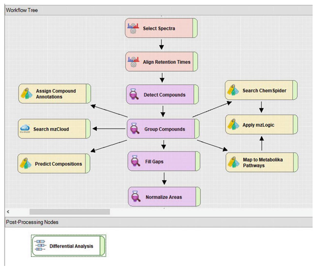
A processing workflow tree. Nodes connected by edges indicate the selected functions for data processing. The workflow represented here is for the workflow template titled “Untargeted Metabolomics with Statistics Detect Unknowns with ID using Online Databases and mzLogic.” The workflow includes retention time alignment, unknown peak detection and ion association, gap filling, detection of background components unrelated to experimental samples, prediction of elemental composition, ChemSpider database searching, mzCloud spectral library matching, pathway mapping, and statistical analysis

Fig. 6.

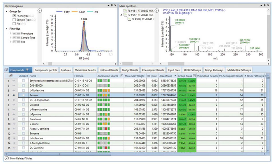
Results page default layout. The Main Table of the Compounds tab includes information for each of the detected compounds including annotation, elemental composition, molecular weight, peak areas, results from database searching and library matching, and univariate statistical results. Selecting a specific compound returns the associated chromatogram overlay and mass spectra

Fig. 7.

Icons in the application toolbar supporting data review. When reviewing a Results File, data review icons are active. Selection of an icon brings the view to the front

Fig. 8.

Recommended minimum peak intensity range for the Detect Compounds node of the Compound Discoverer software. Depending on the mass spectrometer used for data acquisition, corresponding peak intensity values should be selected for unknown peak detection

Box 1. Definitions of Common Terms.

Experimental sample:

Complex biological fluid for LC/MS analysis including human or animal plasma, urine, or CSF.

Pooled sample:

A sample representing multiple experimental samples. The pooled sample is generated by combing the same volume of biofluid from each experimental sample into one stock vial.

Reference metabolite mixture:

A mixture of metabolites in a solvent compatible with the initial LC conditions at low concentration.

Internal standard:

A chemical substance, typically a stable-labeled metabolite, added at a constant amount to each experimental sample used for analytical quality control. Peak area is plotted to visualize variations and potential outliers.

Long-term reference matrix:

A biological sample available in large quantity, which is separate from and not related to the experimental sample used as an analytical reference for LC/MS assessment. Applied to document datapoints over long periods of time for historical record keeping. This reference matrix is often plasma.

References

- 1.Oliver SG, Winson MK, Kell DB, Baganz F (1998) Systematic functional analysis of the yeast genome. Trends Biotechnol 16:373–378 [DOI] [PubMed] [Google Scholar]
- 2.Cho K, Mahieu NG, Johnson SL, Patti GJ (2014) After the feature presentation: technologies bridging untargeted metabolomics and biology. Curr Opin Biotechnol 28:143–148 [DOI] [PMC free article] [PubMed] [Google Scholar]
- 3.Wishart DS (2019) Metabolomics for investigating physiological and pathophysiological processes. Physiol Rev 99:1819–1875 [DOI] [PubMed] [Google Scholar]
- 4.Tebani A, Bekri S (2019) Paving the way to precision nutrition through metabolomics. Front Nutr 6:41. [DOI] [PMC free article] [PubMed] [Google Scholar]
- 5.Nikolskiy I, Siuzdak G, Patti GJ (2015) Discriminating precursors of common fragments for large-scale metabolite profiling by triple quadrupole mass spectrometry. Bioinformatics 31:2017–2023 [DOI] [PMC free article] [PubMed] [Google Scholar]
- 6.Patti GJ (2011) Separation strategies for untargeted metabolomics. J Sep Sci 34:3460–3469 [DOI] [PubMed] [Google Scholar]
- 7.Ivanisevic J, Want EJ (2019) From samples to insights into metabolism: uncovering biologically relevant information in LC-HRMS metabolomics data. Meta 9(12):308. [DOI] [PMC free article] [PubMed] [Google Scholar]
- 8.Patti GJ, Yanes O, Siuzdak G (2012) Innovation: metabolomics: the apogee of the omics trilogy. Nat Rev Mol Cell Biol 13:263–269 [DOI] [PMC free article] [PubMed] [Google Scholar]
- 9.Dunn WB, Bailey NJC, Johnson HE (2005) Measuring the metabolome: current analytical technologies. Analyst 130:606–625 [DOI] [PubMed] [Google Scholar]
- 10.Kind T, Tsugawa H, Cajka T, Ma Y, Lai Z, Mehta SS, Wohlgemuth G, Barupal DK, Showalter MR, Arita M, Fiehn O (2017) Identification of small molecules using accurate mass MS/MS search. Mass Spectrom Rev 37(4):513–532 [DOI] [PMC free article] [PubMed] [Google Scholar]
- 11.Dunn WB, Ellis DI (2005) Metabolomics: current analytical platforms and methodologies. Trends Anal Chem 24(4)285–294 [Google Scholar]
- 12.Mahieu NG, Genenbacher JL, Patti GJ (2016) A roadmap for the XCMS family of software solutions in metabolomics. Curr Opin Chem Biol 30:87–93 [DOI] [PMC free article] [PubMed] [Google Scholar]
- 13.Olivon F, Grelier G, Roussi F, Litaudon M, Touboul D (2017) MZmine 2 data-preprocessing to enhance molecular networking reliability. Anal Chem 89:7836–7840 [DOI] [PubMed] [Google Scholar]
- 14.Lommen A, Kools HJ (2012) MetAlign 3.0: performance enhancement by efficient use of advances in computer hardware. Metabolomics 8:719–726 [DOI] [PMC free article] [PubMed] [Google Scholar]
- 15.Dunn WB, Broadhurst DI, Atherton HJ, Goodacre R, Griffin JL (2011) Systems level studies of mammalian metabolomes: the role of mass spectrometry and nuclear magnetic resonance spectroscopy. Chem Soc Rev 40:387–426 [DOI] [PubMed] [Google Scholar]
- 16.Uppal K, Soltow QA, Strobel FH, Pittard WS, Gernert KM, Yu T, Jones DP (2013) xMSanalyzer: automated pipeline for improved feature detection and downstream analysis of large-scale, non-targeted metabolomics data. BMC Bioinformatics 14:15. [DOI] [PMC free article] [PubMed] [Google Scholar]
- 17.Schwaiger M, Schoeny H, El Abiead Y, Hermann G, Rampler E, Koellensperger K (2019) Merging metabolomics and lipidomics into one analytical run. Analyst 144:220–229 [DOI] [PubMed] [Google Scholar]
- 18.Naser FJ, Mahieu NG, Wang L, Spalding JL, Johnson SL, Patti GJ (2018) Two complementary reversed-phase separations for comprehensive coverage of the semipolar and nonpolar metabolome. Anal Bioanal Chem 410(4):1287–1297 [DOI] [PMC free article] [PubMed] [Google Scholar]
- 19.Contrepois K, Jiang L, Snyder M (2015) Optimized analytical procedures for the untargeted metabolomic profiling of human urine and plasma by combining hydrophilic interaction (HILIC) and reverse-phase liquid chromatography (RPLC)-mass spectrometry. Mol Cell Proteomics 14(6):1684–1695 [DOI] [PMC free article] [PubMed] [Google Scholar]
- 20.Ivanisevic J, Zhu ZJ, Plate L, Tautenhahn R, Chen S, O’Brien PJ, Johnson CH, Marletta MA, Patti GJ, Siuzdak G (2013) Toward ‘omic scale metabolite profiling: a dual separation-mass spectrometry approach for coverage of lipid and central carbon metabolism. Anal Chem 85(14):6876–6884 [DOI] [PMC free article] [PubMed] [Google Scholar]
- 21.Roberts LD, Souza AL, Gerszten RE, Clish CB (2012) Targeted metabolomics. Curr Protoc Mol Biol 98(1):1–34 [DOI] [PMC free article] [PubMed] [Google Scholar]
- 22.Snyder NW, Khezam M, Mesaros CA, Worth A, Blair IA (2013) Untargeted metabolomics from biological sources using ultraperformance liquid chromatography-high resolution mass spectrometry (UPLC-HRMS). J Vis Exp 75:1–8 [DOI] [PMC free article] [PubMed] [Google Scholar]
- 23.Want EJ (2018) LC-MS untargeted analysis. In: Theodoridis AG, Gika HG, Wilson ID (eds) Metabolic profiling, methods and protocols. Humana, New York, NY, pp 99–116 [Google Scholar]
- 24.University of California San Diego. Metabolomics workbench, general protocols. https://www.metabolomicsworkbench.org/protocols/general.php. Accessed 12 Jan 2019
- 25.European Molecular Biology Laboratory (2019) Metabolomics core facility, protocols used for LC-MS analysis. https://www.embl.de/mcf/metabolomics-core-facility/protocols/. Accessed 12 Jan 2019
- 26.Saigusa D, Okamura Y, Motoike IN, Katoh Y, Kurosawa Y, Saijyo R, Koshiba S, Yasuda J, Motohashi H, Sugawara J, Tanabe O, Kinoshita K, Yamamoto M (2016) Establishment of protocols for global metabolomics by LC-MS for biomarker discovery. PLoS One 11(8):e0160555. [DOI] [PMC free article] [PubMed] [Google Scholar]
- 27.Gika HG, Zisi C, Theodoridis G, Wilson ID (2016) Protocol for quality control in metabolic profiling of biological fluids by U(H)PLC-MS. J Chromatogr B Anal Technol Biomed Life Sci 1008:15–25 [DOI] [PubMed] [Google Scholar]
- 28.Knee JM, Rzezniczak TZ, Barsch A, Guo KZ, Merritt TJS (2013) A novel ion pairing LC/MS metabolomics protocol for study of a variety of biologically relevant polar metabolites. J Chromatogr B Anal Technol Biomed Life Sci 936:63–73 [DOI] [PubMed] [Google Scholar]
- 29.Esterhuizen K, van der Westhuizen FH, Louw R (2017) Metabolomics of mitochondrial disease. Mitochondrion 35:97–110 [DOI] [PubMed] [Google Scholar]
- 30.Barshop BA (2004) Metabolomic approaches to mitochondrial disease: correlation of urine organic acids. Mitochondrion 4:521–527 [DOI] [PubMed] [Google Scholar]
- 31.Shaham O, Slate NG, Goldberger O, Xu Q, Ramanathan A, Souza AL, Clish CB, Sims KB, Mootha VK (2010) A plasma signature of human mitochondrial disease revealed through metabolic profiling of spent media from cultured muscle cells. Proc Natl Acad Sci U S A 107(4):1571–1575 [DOI] [PMC free article] [PubMed] [Google Scholar]
- 32.Leoni V, Strittmatter L, Zorzi G, Zibordi F, Dusi S, Garavaglia B, Venco P, Caccia C, Souza AL, Deik A, Clish CB, Rimoldi M, Ciusani E, Bertini E, Nardocci N, Mootha VK, Tiranti V (2012) Metabolic consequences of mitochondrial coenzyme A deficiency in patients with PANK2 mutations. Mol Genet Metab 105(3):463–471 [DOI] [PMC free article] [PubMed] [Google Scholar]
- 33.Yao CH, Wang R, Wang Y, Kung CP, Weber JD, Patti GJ (2019) Mitochondrial fusion supports increased oxidative phosphorylation during cell proliferation. Elife 8:pii:e41351 [DOI] [PMC free article] [PubMed] [Google Scholar]
- 34.Mandal R, Chamot D, Wishart DS (2018) The role of the Human Metabolome Database in inborn errors of metabolism. J Inherit Metab Dis 41:329–336 [DOI] [PubMed] [Google Scholar]
- 35.Feuchtbaum L, Carter J, Dowray S, Currier RJ, Lorey F (2012) Birth prevalence of disorders detectable through newborn screening by race/ethnicity. Genet Med 14:937–945 [DOI] [PubMed] [Google Scholar]
- 36.Thermo Fisher Scientific, Exactive Series Operating Manual, BRE0012255, Revision A, April 2017. https://assets.thermofisher.com/TFS-Assets/CMD/manuals/man-bre0012255-exactive-series-manbre0012255-en.pdf. Accessed 16 Feb 2019
- 37.Tsugawa H, Cajka T, Kind T, Ma Y, Higgins B, Ikeda K, Kanazawa M, VanderGheynst J, Fiehn O, Arita M (2015) MS-DIAL: data-independent MS/MS deconvolution for comprehensive metabolome analysis. Nat Methods 12:523–526 [DOI] [PMC free article] [PubMed] [Google Scholar]
- 38.Chong J, Soufan O, Li C, Caraus I, Li S, Bourque G, Wishart DS, Xia J (2018) MetaboAnalyst 4.0: towards more transparent and integrative metabolomics analysis. Nucleic Acids Res 46:W486–W494 [DOI] [PMC free article] [PubMed] [Google Scholar]
- 39.Mahieu NG, Spalding J, Patti GJ (2015) Warpgroup: increased precision of metabolomic data processing by consensus integration bound analysis. Bioinformatics 32:268–275 [DOI] [PMC free article] [PubMed] [Google Scholar]
- 40.Blazenovic I, Kind T, Ji J, Fiehn O (2018) Software tools and approaches for compound identification of LC-MS/MS data in metabolomics. Meta 8(2):31. [DOI] [PMC free article] [PubMed] [Google Scholar]
- 41.Stanstrup J, Broeckling CD, Helmus R, Hoffmann N, Mathe E, Naake T, Nicolotti L, Peters K, Rainer J, Salek RM, Schulze T, Schymanski EL, Stravs MA, Thevenot EA, Treutler H, Weber RJM, Willighagen E, Witting M, Neumann S (2019) The metaRbolomics toolbox in bioconductor and beyond. Meta 9(10):200. [DOI] [PMC free article] [PubMed] [Google Scholar]
- 42.Souza A, Tautenhan R (2018) Features or compounds? A data reduction strategy for untargeted metabolomics to generate meaningful data (Report no. TN65204-EN 0418S). Thermo Fisher Scientific. https://assets.thermofisher.com/TFS-Assets/CMD/Technical-Notes/tn-65204-lc-ms-untargeted-metabolomics-tn65204-en.pdf. Accessed 16 Feb 2020 [Google Scholar]
- 43.Mahieu NG, Patti GJ (2017) Systems-level annotation of a metabolomics data set reduces 25000 features to fewer than 1000 unique metabolites. Anal Chem 89:10397–10406 [DOI] [PMC free article] [PubMed] [Google Scholar]
- 44.Fiehn O, Robertson D, Griffin J, van der Werf M, Nikolau B, Morrison N, Sumner LW, Goodacre R, Hardy NW, Taylor C, Fostel J, Kristal B, Kaddurah-Daouk R, Mendes P, van Ommen B, Lindon JC, Sansone S (2007) The metabolomics standards initiative (MSI). Metabolomics 3:175–178 [Google Scholar]
- 45.Sumner LW, Amberg A, Barrett D, Beale MH, Beger RD, Daykin CA, Fan T, Fiehn O, Goodacre R, Griffin JL, Hankemeier T, Hardy NW, Harnly J, Higashi RM, Kopka J, Lane AN, Lindon JC, Marriott P, Nicholls AW, Reily MD, Thaden J, Viant M (2007) Proposed minimum reporting standards for chemical analysis. Metabolomics 3:231–241 [DOI] [PMC free article] [PubMed] [Google Scholar]
- 46.Souza A, Ntai I, Tautenhan R (2018) Accelerated unknown compound annotation with confidence: from spectra to structure in untargeted metabolomics experiments (Report no. AN65362-EN 1218M). Thermo Fisher Scientific. https://assets.thermofisher.com/TFS-Assets/CMD/Application-Notes/an-65362-ms-compound-annotation-an65362-en.pdf. Accessed 16 Feb 2020 [Google Scholar]