Whole‐brain high‐resolution metabolite mapping with 3D compressed‐sensing SENSE low‐rank ¹H FID‐MRSI

Abstract

There is a growing interest in the neuroscience community to map the distribution of brain metabolites in vivo. Magnetic resonance spectroscopic imaging (MRSI) is often limited by either a poor spatial resolution and/or a long acquisition time, which severely restricts its applications for clinical and research purposes. Building on a recently developed technique of acquisition‐reconstruction for 2D MRSI, we combined a fast Cartesian ¹H‐FID‐MRSI acquisition sequence, compressed‐sensing acceleration, and low‐rank total‐generalized‐variation constrained reconstruction to produce 3D high‐resolution whole‐brain MRSI with a significant acquisition time reduction. We first evaluated the acceleration performance using retrospective undersampling of a fully sampled dataset. Second, a 20 min accelerated MRSI acquisition was performed on three healthy volunteers, resulting in metabolite maps with 5 mm isotropic resolution. The metabolite maps exhibited the detailed neurochemical composition of all brain regions and revealed parts of the underlying brain anatomy. The latter assessment used previous reported knowledge and a atlas‐based analysis to show consistency of the concentration contrasts and ratio across all brain regions. These results acquired on a clinical 3 T MRI scanner successfully combined 3D ¹H‐FID‐MRSI with a constrained reconstruction to produce detailed mapping of metabolite concentrations at high resolution over the whole brain, with an acquisition time suitable for clinical or research settings.

A novel acquisition‐reconstruction scheme, combining FID‐MRSI with a compressed‐sensing sensitivity‐encoding low‐rank model, makes possible 3D spectroscopic imaging of the whole human brain in high resolution on a 3 T system. Following 20 min acquisition, the resulting metabolic maps reflect the detailed neurochemical composition of all brain regions.

Abbreviations used

¹H‐MRSI

proton magnetic resonance spectroscopic imaging

Cho

choline moiety metabolites

CRLB

Cramer‐Rao lower bound

CS

compressed sensing

CS‐SENSE‐LR

compressed‐sensing sensitivity‐encoding low‐rank

FID

free induction decay

Glx

glutamate + glutamine

GM

gray matter

HSVD

Hankel singular value decomposition

Ins

myo‐inositol

I.U.

institutional unit

MM

macromolecule

OVS

outer‐volume saturation bands

RMS

root mean square

RMSE

normalized root mean square error

SNR

signal‐to‐noise ratio

SSE

spatio‐spectral encoding

SSIM

structural similarity index

tCre

creatine + phosphocreatine

TE

echo time

TGV

total generalized variation

tNAA

N‐acetylaspartate + N‐acetylaspartylglutamate

TR

repetition time

VOI

volume of interest

WET

water suppression enhanced through T ₁ effects

WM

white matter

1. INTRODUCTION

Measuring metabolite distributions in three dimensions over the whole human brain using proton magnetic resonance spectroscopic imaging (¹H‐MRSI) has been the subject of two decades of intense research. From early multi‐slice methods ¹ , ² covering a large portion of the brain to the first development of spatio‐spectral encoding (SSE) techniques ³ , ⁴ , ⁵ proposed by Mansfield, ⁶ whole brain ¹H‐MRSI has unraveled distributions with unique patterns for each metabolite and provided original physiological information that complements the usual MR imaging. Since then, 3D ¹H‐MRSI methods for human brain imaging have been improved by implementing acceleration techniques ⁷ , ⁸ , ⁹ or significant increase in spatial resolution. ¹⁰ , ¹¹ A more complete overview of ¹H‐MRSI techniques can be found in review articles. ¹² , ¹³ , ¹⁴

Recently, advances in reconstruction methods have provided new solutions to the inherent limitations of ¹H‐MRSI. The ¹H‐MRSI acquisition geometry is often restricted to a rectangular volume of interest (VOI) with saturation of the outer signal to prevent skull lipid contamination. However, recent work on efficient post‐acquisition lipid decontamination ¹⁵ , ¹⁶ , ¹⁷ , ¹⁸ enables the measurement of whole brain slices without limited VOI by in plane selective excitation. In addition, employing models with constraints of prior information for ¹H‐MRSI data reconstruction significantly improves spectral quality and the resulting metabolite distributions. ¹⁹ , ²⁰ A priori knowledge of the underlying signal can also be exploited for super‐resolution ²¹ , ²² or drastic acceleration of ¹H‐MRSI acquisition. ²³ , ²⁴

Acquisition of whole‐brain MRSI using traditional methods could be particularly lengthy due to the necessity to encode the large 4D k‐t space. However, acquisition time can be significantly reduced by using several techniques such as free induction decay (FID)‐MRSI acquisition, parallel imaging, and compressed sensing (CS). The FID‐MRSI sequence, first known for its application in spectroscopic imaging of ³¹P and other nuclei, ²⁵ , ²⁶ has been more recently proposed for ¹H‐MRSI. ²⁷ , ²⁸ The simple sequence design dramatically shortens the acquisition time compared with usual spin‐echo methods by allowing low‐flip‐angle excitation and sub‐second repetition time (TR). Implementing parallel imaging techniques in 3D ¹H‐MRSI of the human brain can reduce the acquisition time by a factor of 2 to 8. ⁸ , ⁹ , ²⁹ Following the recent developments of CS for MRI, ³⁰ , ³¹ the sparsity present in the 3D MRSI signal can also be exploited to accelerate the encoding of the 4D k‐t space. The effectiveness of this approach was demonstrated for ¹³C and ¹⁹F ³² , ³³ as well as in combination with fast spatial‐spectral encoding. ³⁴ Applying CS to ¹H‐MRSI of the human brain grants accelerations up to a factor of 4, but has been limited to 2D acquisitions so far. ¹⁷ , ³⁵ , ³⁶ , ³⁷ , ³⁸

State‐of‐the‐art techniques offering 3D whole‐brain ¹H‐MRSI often rely on the use of SSE, ¹⁴ which uses entire lines to encode the 4D k‐t space. Hence, these approaches allow highly accelerated acquisitions and permit MRSI acquisitions of the whole brain in high resolution within a duration compatible with clinical requirements. The trajectory can be either echo‐planar, ²⁴ , ³⁹ concentric circles, ¹⁰ , ⁴⁰ rosette, ⁴¹ or spiral. ⁴² With a signal‐to‐noise ratio (SNR)/time comparable to Cartesian encoding of same resolution, ¹⁴ then SSE technique might nevertheless result in low‐SNR data that require averaging or specific denoising model‐based approaches. ²⁴ The method of acceleration presented hereafter relies on undersampling of the Cartesian 3D k‐space. The non‐linear reconstruction process ¹⁷ is expected to preserve SNR or to result in a slower decrease as function of the acceleration factor. On the other hand, high acceleration is expected to affect the spatial distributions of the MRSI signal, as pointed out in previous studies of CS with MRI. ⁴³ , ⁴⁴ In this study, we aim to evaluate the capability of the proposed framework as an alternative to the acceleration of 3D MRSI with SSE.

We present original results of high‐resolution 3D ¹H‐MRSI of the whole human brain on a 3 T clinical system. The acquisition‐reconstruction scheme combines a fast FID‐MRSI high‐resolution sequence accelerated by random undersampling and reconstructed with a CS sensitivity‐encoding low‐rank model (CS‐SENSE‐LR) ¹⁷ extended to 3D. This comprehensive approach, combining FID and parallel acquisition schemes with CS‐SENSE‐LR reconstruction, aims to drastically shorten the acquisition time and allows the implementation of high‐resolution 3D MRSI in clinical and research scanning protocols. High‐resolution metabolite mapping will have a great range of applications from neurology to psychiatry. ⁴⁵ , ⁴⁶ In clinical neuroscience and with usual spectroscopic techniques, interpretation of spectroscopy findings is limited by the VOI approach, neglecting large cerebral parts around the volume selected by the a priori hypothesis. There is a strong need for whole‐brain spectroscopic imaging, which allows not only the mapping of metabolites in all brain regions but also the integration of brain spectroscopic data with other imaging modalities including structural and diffusion MR. ⁴⁷

2. METHODS

2.1. Sequence and acquisition

A ¹H‐FID‐MRSI ²⁷ , ²⁸ sequence with a 3D phase encoding was implemented (Figure 1) on a 3 T Prisma fit MRI (Siemens, Erlangen, Germany) using a receiver head coil with $N_{\mathrm{c}}=$ 64 elements. A Shinnar‐LeRoux optimized slab‐selective excitation pulse of 0.9 ms was used with a 9.5 kHz bandwidth. Water suppression enhanced through T ₁ effects (WET), ⁴⁸ was implemented using three Gaussian pulses with 60 Hz bandwidth and separated by 20 ms each. The acquisition delay between the excitation and the signal acquisition was minimized to an echo time (TE) of 0.65 ms. A 4 kHz sampling rate FID was acquired with $T=$ 1024 points followed by spoiler gradients for a TR of 355 ms. To avoid signal saturation considering the maximum T ₁ value among metabolite to be 1400 ms, ⁴⁹ the excitation flip angle was set to 35°. To avoid aliasing from signal outside the slab, two 30‐mm‐thick outer‐volume saturation bands (OVS) were positioned directly below and above the slab. The excited slab size was (A/P‐R/L‐H/F) 210 mm by 160 mm by 95 mm. The 3D encoding volume was set slightly larger, to 210 mm by 160 mm by 105 mm, again to prevent aliasing. An encoding matrix of 42 × 32 × 20 resulted in a 131 μ L voxel volume (5 mm isotropic). A fast reference water measurement was performed to determine the coil sensitivity profiles, with acquisition parameters identical to the main FID‐MRSI sequence but without WET and with lower resolution, 32 × 24 × 16 (6.6 mm isotropic). The same encoding volume and slab were used but with 31 ms TR, 48 points in FID and a 5° flip angle. An anatomical 3D T ₁‐weighted MPRAGE sequence was also acquired during the session for navigation purposes and for anatomical segmentation of the volunteers' brains.

FIGURE 1.

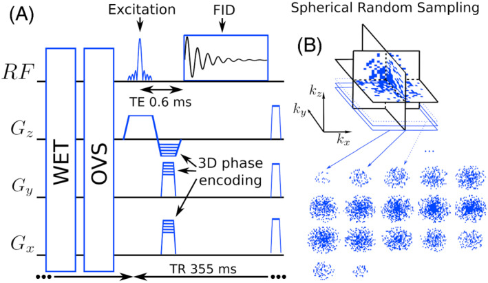
Left, schematic of the FID‐MRSI sequence with 3D phase encoding preceded by the WET and OVS sequence blocks. Right, an example of 3D k‐space undersampled by a factor of 3.5

2.1.1. Sparse and random 3D phase encoding

MRSI raw data were acquired sparsely and randomly over the 3D Fourier domain (k‐space) to enable CS acceleration. The sequential phase‐encoding method of the FID‐MRSI sequence allows for a straightforward implementation of the random k‐space sampling. During sequence preparation, a 3D mask was computed containing only k‐space coordinates to be acquired. Defining $q=\sqrt{{(k_x/k_x^{\max })}^2+{(k_y/k_y^{\max })}^2+{(k_z/k_z^{\max })}^2}$, the random sampling of the 3D mask was constrained to a density distribution following q ⁻¹ but with a fully sampled spheroid of radius $q\le \frac{1}{5}$ (Figure 1). During the sequence acquisition, following the preparation, FID‐MRSI data were acquired according to the 3D k‐space mask.

2.2. MRSI data preprocessing and reconstruction model

2.2.1. Remaining water and lipid signal removal

Residual water was removed using the Hankel singular value decomposition (HSVD) method. ⁵⁰ HSVD was applied separately to each coil element and time series in the acquired points of the k‐space. The lipid suppression was performed in k‐space on the signal from each coil element using a lipid subspace projection method ¹⁷ based on the metabolite‐lipid spectral orthogonality hypothesis. ¹⁵ The computation time of the residual water removal was below 60 min while the lipid suppression was computed within 2 min using MATLAB R2018b (MathWorks, Natick, Massachusetts) and a 16‐core 3.00 GHz Intel Xeon‐E5 CPU. The methods are described in detail in previously published work. ¹⁷

2.2.2. CS‐SENSE‐LR reconstruction

The CS approach requires reconstruction of the sparsely sampled MRSI data with an appropriate model that maximizes data fidelity while constraining spatial sparsity in metabolite distributions. ³⁰ , ³¹ We employed here a low‐rank constrained model that includes total generalized variation (TGV) regularization. ⁵¹ We briefly describe hereafter the 3D extension of the CS‐SENSE‐LR reconstruction that was previously described. ¹⁷ MRSI raw data measured by phased array coil element $c=1,\dots ,N_{\mathrm{c}}$ at time t and at k‐space coordinate k can be expressed with the forward model

$$s_c(\mathbf{k},t)={\int }_{\Omega \subset {ℝ}^3}{\mathrm{e}}^{2\pi \mathrm{i}\mathbf{k}·\mathbf{r}}{C}_c(\mathbf{r})B(\mathbf{r},t)\rho (\mathbf{r},t)d\mathbf{r},$$ (1)

with 3D spatial coordinates r integrated over Ω, the spatial support of the measured object, and $\rho (\mathbf{r},t)\in ℂ$ the transverse magnetization. $C_c(\mathbf{r})\in ℂ$ represent the coil sensitivity profiles and $B(\mathbf{r},t)={\mathrm{e}}^{2\pi \mathrm{i}t\gamma \mathrm{\Delta }{B}_0(\mathbf{r})}$ the spatial frequency shift caused by γΔB ₀(r), the magnetic field inhomogeneity map (in Hz). The goal of the reconstruction is to retrieve the original ρ(r, t) from the sparsely sampled signal s _c (k, t) knowing C _c (r) and ΔB ₀(r).

The low‐rank assumption implies a decomposition of the transverse magnetization in K spatial and temporal components, $U_n(\mathbf{r}),V_n(t),n=1,\dots ,K$:

$$\begin{array}{cc}\hfill \rho (\mathbf{r},t)=& {\displaystyle \sum _{n=1}^K}{U}_n(\mathbf{r})V_n(t)\hfill \\ \hfill =& \mathbf{U}(\mathbf{r})\mathbf{V}(t),\hfill \end{array}$$ (2)

with the last line employing vectorial notation. Considering discrete spatial and temporal sampling points (N _t time points, N _k k‐space acquisition points, N _x , N _y , N _z the reconstruction image size), s _c (k, t), U(r), V(t) become multi‐dimensional arrays s, U, V with size respectively (N _c × N _k  × N _t ), (N _x  × N _y  × N _z  × K) and (K × N _t ). The forward model (1) then reads

$$\mathbf{s}=\mathcal{F}\mathcal{C}\mathcal{B}(\mathbf{U}\mathbf{V}),$$ (3)

with the discrete Fourier transform operator $\mathcal{F}$, and $\mathcal{C}$ and $\mathcal{B}$ operators applying C _c (r) and B(r, t) on discrete coordinates. First, remaining water and lipid signals are removed from s as described above in previous section. Second, the magnetization in image space $\mathit{\rho }=\mathbf{U}\mathbf{V}$ is reconstructed from s with a 3D low‐rank TGV model. The TGV minimization problem ⁵¹ , ⁵² enables the determination of the spatial and temporal components

$$\arg \underset{\mathbf{U}\mathbf{V}}{\min }{‖\mathbf{s}-\mathcal{F}\mathcal{C}\mathcal{B}(\mathbf{U}\mathbf{V})‖}_2^2+\lambda {\displaystyle \sum _{n=1}^K}{\text{TGV}}^2\{U_n\}.$$ (4)

The coil sensitivity profiles C _c (r) were determined from the fast reference water acquisition using ESPIRiT, ⁵³ and ΔB ₀(r) was estimated using the multiple signal classification algorithm (MUSIC) ⁵⁴ on the water signal from the same fast reference scan. By including coil sensitivity profiles and the TGV regularization that imposes sparsity in spatial first‐ and second‐order gradients, the CS‐SENSE‐LR reconstruction permits a faithful reconstruction of randomly sampled MRSI data. ⁴³ , ⁵⁵ As a consequence of the sequence design, there is a delay between the excitation and the FID acquisition that causes a first‐order phase in the reconstructed spectra. To correct this effect, the first two missing points of the FID were estimated using a reverse autoregressive model ⁵⁶ in each voxel of the reconstructed MRSI dataset $\mathit{\rho }=\mathbf{U}\mathbf{V}$ individually. The MRSI reconstruction including all pipeline steps takes approximately 12 h to complete using MATLAB R2018b and a workstation with a 16‐core 3.00 GHz Intel Xeon‐E5 CPU.

2.2.3. LCModel quantification

In a last step, the reconstructed MRSI signal was fitted with LCModel ⁵⁷ , ⁵⁸ to quantify metabolites voxel by voxel over the range of 1.0 to 4.2 ppm. The LCModel basis was simulated using the GAMMA package ⁵⁹ and with parameters matching the acquisition sequence. The metabolites in the basis included N‐acetylaspartate, N‐acetyl aspartylglutamate, creatine, phosphocreatine, glycerophosphocholine, phosphocholine, myo‐inositol, scyllo‐inositol, glutamate, glutamine, lactate, gamma‐aminobutyric acid, glutathione, taurine, aspartate, and alanine. LCModel results were expressed in institutional units (I.U.), which allow for comparison across metabolites and subjects (see LCModel documentation ⁵⁸ ). Although an absolute quantification of the metabolite signal would be possible with the proposed acquisition‐reconstruction scheme, it would require multiple additional correction and adjustment factors, such as tissue specific T ₁ corrections, water content correction, and transmit amplitude for body and phased‐array coils. ⁶⁰ , ⁶¹ It is however possible to give an estimate of the scaling between the I.U. and the metabolite concentrations in millimolar. If we assume that T ₁ of the metabolites and the water is 1200 ms, and that the water concentration is 42.98 mM in the whole brain, ⁶¹ we can approximate that $1\text{I.U}.\approx 3.2\text{mM}$ for all the data reported in this paper.

Lipid suppression by orthogonality as performed in this study might distort the baseline at 2 ppm below the NAA singlet peak. To optimize LCModel fitting in the presence of this distortion a singlet broad and inverse peak was added to the basis. It was simulated at 2 ppm with 20 Hz width and an e^iπ phase (opposite to the NAA singlet). LCModel quantification provides also estimates of spectrum SNR and a Cramer‐Rao lower bound (CRLB) for each metabolite. These are usually considered as spectral quality metrics, but, for the present results reconstructed with the CS‐SENSE‐LR model prior to the LCModel fitting, these parameters might not assess data quality properly, especially as the accurate estimation of these parameters relies on the presence of measurement noise within the spectra. In the present work, the measurement noise is removed by using the denoising model. Therefore, CRLB values might be artificially low and SNR particularly high. Nevertheless, as they still reflect the fitting quality, they are provided in the Supporting Information. Instead, the average of the LCModel fit residuals is reported to describe spectral quality.

2.3. Experiments

2.3.1. Assessing CS acceleration

To demonstrate the CS acceleration capability and to assess the metabolite map reconstruction accuracy, a single MRSI acquisition without k‐space undersampling was performed on a volunteer using the sequence details in section 2.1 with a full elliptical k‐space encoding, resulting in a 70 min acquisition. The raw data were first undersampled retrospectively to various extents to reproduce acceleration factors of 2, 3, 4, 5 or 6 and following the same variable density undersampling as the actual accelerated acquisition (described in section 2.1). After undersampling of the raw data, metabolite maps were reconstructed following all the steps from section 2.2. The TGV regularization parameter λ in (4) was adjusted on the fully sampled dataset (3 × 10⁻⁴) and was kept the same for all acceleration factors. The reconstructed spectral quality was assessed at different accelerations and the fitting residuals of the LCModel were quantified as a quality parameter. The resulting metabolite maps were compared qualitatively and quantitatively with a normalized root mean square error (RMSE) and structural similarity index (SSIM).

2.3.2. Accelerated acquisition on healthy volunteers

The FID‐MRSI with accelerated acquisition was performed and reconstructed with the CS‐SENSE‐LR model on three healthy volunteers to demonstrate reproducibility and robustness. Written informed consent was given by all the volunteers before participation, and the study protocol was approved by the institutional ethics committee. The FID‐MRSI was acquired with an acceleration factor of 3.5 (20 min, optimal factor determined by assessing CS acceleration) for all three volunteers and was reconstructed with the same regularization as the retrospective acceleration case, ie $\lambda =3\times 10^{-4}$. The spectral quality was presented with selected reconstructed spectra from four locations: the cingulate gray matter (GM), the frontal white matter (WM), the caudate nucleus and the temporal GM with the corresponding LCModel fitting.

2.3.3. Brain‐atlas regional analysis

To illustrate the metabolite contrasts and their relation to the underlying anatomical structures, the 3D metabolite maps were co‐registered to an anatomical brain atlas. For each participant, T ₁‐weighted anatomical scans were segmented into GM and WM compartments by using the computational anatomy toolbox (CAT12; http://www.neuro.uni-jena.de/cat). Masks for the cerebral lobes were generated using the Standard atlas ⁶² in the WFU_PickAtlas toolbox (https://www.nitrc.org/projects/wfu_pickatlas/) and subcortical GM structures were automatically segmented using FreeSurfer version 6.0.0. ⁶³ To cope with MRSI partial voluming, a general linear model was employed to fit the metabolite concentration in each anatomical structure (a detailed description of the model is given in the Supporting Information). These values were computed for all three volunteers, and the mean ratios $\left(\frac{\text{tNAA}}{\text{tCre}},\frac{\text{Cho}}{\text{tCre}},\frac{\text{Ins}}{\text{tCre}},\frac{\text{Glx}}{\text{tCre}}\right)$ across volunteers were compared with reported values. ⁶⁰ , ⁶⁴ , ⁶⁵ , ⁶⁶ , ⁶⁷ An ANOVA was performed for each metabolite across anatomical structures with the three volunteers' data to highlight significant differences in metabolite concentration. Following this test, a multiple comparison was performed to investigate possible significant pairwise differences between individual structures.

3. RESULTS

The results of the in vivo MRSI data accelerated retrospectively to illustrate the CS performance are shown in Figure 2 for the five major metabolites measured: N‐acetylaspartate + N‐acetyl aspartylglutamate (tNAA), creatine + phosphocreatine (tCre), choline moiety metabolites (Cho) (choline, acetylcholine, phosphocholine and glycerophosphocholine), myo‐inositol (Ins), and glutamate + glutamine (Glx). The cortical layer is visible on tCr and Glx maps and the Cho distribution shows the highest signal intensity in frontal WM and the lowest values in the occipital lobe. These spatial features remain clear even when data are progressively randomly undersampled in the k‐space from 50% to 17% (acceleration factor from 2 to 6). Although all datasets were reconstructed with the same regularization parameter value λ, metabolite images gradually lose fine detailed structures and show blurriness as the acceleration factor increases, due to the lack of high k‐space frequencies remaining sampled in the data. This is highlighted by the generally monotonic rise of RMSE and decrease of SSIM. A thorough simulation of image reconstruction was performed to demonstrate this effect (results are presented in the Supporting Information). It is demonstrated that a regularized model with optimal parameter minimizes the reconstruction error, whereas a strong acceleration of the data cannot be reliably reconstructed without important loss of apparent resolution.

FIGURE 2.

Top, 3D FID‐MRSI reconstructed metabolite volumes with retrospective acceleration. The fully sampled acquisition (No acceleration) was acquired in 70 min and acceleration factors correspond to k‐space undersampling and reducing acquisition time accordingly (e.g. ×3, 24 min; ×6, 12 min). The color map was scaled individually for each metabolite range from 0 to the 95th percentile. Bottom, the normalized RMSE and SSIM computed for each metabolite map at all acceleration factors relative to the unaccelerated result. Sample spectra from two distinct locations are displayed and exhibit very little variation with the acceleration (no, 3, 5). The LCModel fits are shown with the fitting residuals. Bottom left, the RMS of the residuals averaged over the whole brain remains constant with the acceleration

The RMSE and SSIM of each metabolite volume relative to the 'no acceleration' volume show monotonic behaviors close to a linear relation with the acceleration factor in agreement with previous publications. ³⁸ , ⁵⁵ Among all metabolites Glx consistently shows the highest RMSE and lowest SSIM. This is probably due to the lower signal of glutamine and glutamate compared to other metabolites. tNAA also shows higher error and lower similarity in comparison with tCre or Cho. This is possibly related to the lipid suppression that can affect baseline at 2 ppm and add variability to the tNAA quantification.

Spectra shown for two locations at the bottom of Figure 2 exhibit no noticeable change with acceleration. Possible spectral distortion as a result of the acceleration could induce an increase of fitting residuals; however, the residual root mean square (RMS) average over the brain remains relatively constant.

The full tNAA, tCre, Cho, Ins, and Glx maps resulting from the accelerated acquisition (i.e. 3.5) are displayed for Volunteer 1 in Figure 3. The metabolite maps match the distribution features and have similar quality as for the retrospective acceleration by a factor 3 or 4 in Figure 2. Volumes of Cho and Glx concentrations that display the sharpest contrasts, and four sample spectra, are presented in Figure 4 for each of the three volunteers. The concentration variations observed in the metabolite maps translate into visual spectral variations. The frontal WM spectrum shows a clear higher Cho peak with respect to the other three locations, and the cingulate GM and temporal GM spectra present markedly higher Glx signal than the frontal WM and caudate. These visual landmarks are noticeable for all three volunteers. The metabolite concentration ratio maps of the same measurements are shown in Supporting Information Figure S9. In addition, CRLB and SNR maps of these results are presented in Supporting Information Figure S10 but should be interpreted with caution. Indeed, their accuracy might be affected by the reconstruction process as described in the Methods. To validate the quantification in I.U. with respect to the water reference signal, MRSI data were measured, reconstructed and quantified on a homogeneous metabolite solution phantom (MRS Braino phantom, GE Medical Systems, Milwaukee, Wisconsin). The resulting metabolite map (Supporting Information Figure S16) exhibits homogeneity over the whole phantom.

FIGURE 3.

CS‐SENSE‐LR 3D FID‐MRSI measured on a healthy volunteer (Volunteer 1) with 5 mm isotropic resolution in 20 min with acceleration factor 3.5 resulted in tNAA, tCre, Cho, Ins, and Glx maps. The color scale for each map is given in I.U. The sagittal T ₁‐weighted image (bottom right) shows the location of the excitation slab (blue overlay)

FIGURE 4.

Comparison of high‐contrast Cho and Glx 3D maps measured with CS‐SENSE‐LR FID‐MRSI on three healthy volunteers (Volunteers 1, 2, and 3) with 5 mm isotropic resolution in 20 min (acceleration factor 3.5). The color scale is given in I.U. for the respective metabolite concentrations. Sample spectra originating from four distinct locations are shown for each volunteer. Cho and Glx signal amplitudes in the spectra match the metabolite distribution observable on the maps. Metabolite ratio maps of the same volunteers and the corresponding CRLB and SNR maps estimated using LCModel are shown in Supporting Information Figure S10

The spectra shown in Figures 4 and 2 exhibit high SNR as a result of the low‐rank constraint and a narrow linewidth due to the small voxel size as well as the B ₀ field‐map correction included in the CS‐SENSE‐LR model. The mean whole‐brain SNR estimated using LCModel was 14.2, 12.7, and 12.6 and the mean spectral full width at half maximum was 5.67 Hz, 5.46 Hz, and 5.19 Hz for Volunteers 1 to 3, respectively. The baseline distortion due to the lipid suppression by orthogonality is visible as a pit at 2 ppm, forming a ‘W’ shape with the NAA peak. Nevertheless, the distortion is well fitted by the inverse broad peak added to the basis and the resulting baseline is smooth. The metabolite maps remain sensitive to B ₀‐field inhomogeneity, which results in local linewidth increase. This effect is visible in the lower sections of the metabolite maps, B ₀ field maps and linewidth maps (Figure 4, Supporting Information Figures S12 and S11).

The anatomical segmentation of 3D metabolite maps for Volunteer 1 is illustrated in Figure 5. Concentrations of each anatomical region are reported in Figure 6 and illustrate the consistency of the anatomical contrasts for all volunteers, with the distribution of metabolite concentrations following similar patterns. For tNAA, cortical concentrations tend to be lower in temporal lobes while subcortical concentrations are relatively high in the thalamus. Similarly, tCre concentrations are lower in temporal lobes than in other cortical regions. There is also a systematic difference in tCre between GM and WM. For Cho, plots show a lower concentration in GM than in WM as well as a high concentration in the brain stem, hippocampus, and amygdala. In contrast to Cho, Glx exhibits a consistent and markedly higher concentration in GM than in WM. The distribution of Ins concentrations follows a GM‐WM contrast similar to tCre. The cerebellum is marked by high concentrations of tCre, Glx, and Ins. The ratios of metabolite concentrations in each anatomical region, averaged across subjects, are presented in Figure 7. Values from the left and right hemispheres were combined to facilitate comparison with results from the literature. ⁶⁰ , ⁶⁴ , ⁶⁵ , ⁶⁶ , ⁶⁷ Globally, results for tNAA/tCre, Cho/tCre, and Glx/tCre match the previously reported ratio values, with differences that are in the range of what has been previously published, although tNAA/tCre and Cho/tCre values are among the highest reported values and Glx/tCre among the lowest. The GM‐WM contrast that is reported in the literature for all metabolite ratios is also observed in the present study. Ins/tCre values are systematically larger than the literature results, although the GM‐WM contrast here is comparable. Results of the statistical analyses of differences across brain regions are presented in Supporting Information Figure S15. The ANOVA exhibited a significant difference across regions in all the metabolites (p‐value given in the title of each figure). The results of the multiple comparison testing are presented as matrices for each metabolite. Significant differences (corrected p < 0.05) are consistent with the qualitative results described above. Cerebellum concentration is significantly higher compared with various other structures for tCre, Cho, and Glx. The cortical GM regions are significantly different from WM and deep GM structures regarding Glx and tCre. Ins and tNAA show fewer significant differences between deep GM structures or between deep GM structures and lobe values.

FIGURE 5.

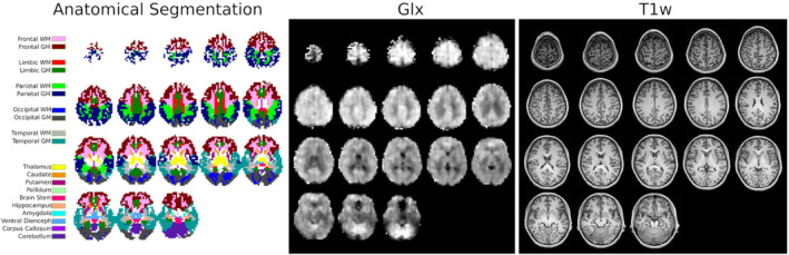
Left, the anatomical atlas registered to Volunteer 1 is shown with voxel labeling corresponding to the dominant partial volume. Center, the Glx concentration 3D map is shown for qualitative comparison in a gray scale. Right, the MPRAGE T ₁‐weighted images used to segment the volunteer anatomic parts

FIGURE 6.

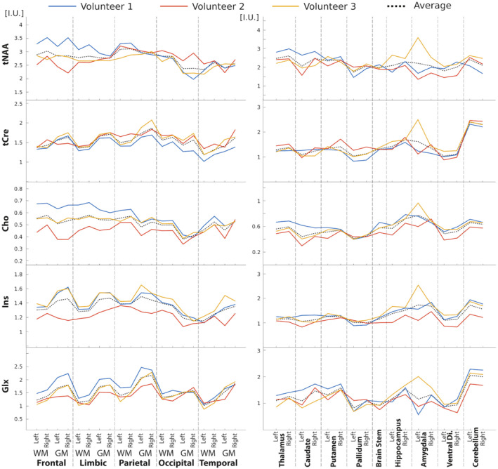
Atlas metabolite content across three healthy volunteers based on anatomical segmentation (Figure 5). Lines correspond to the metabolite concentration estimated for all anatomical area for each of the three volunteers. The dashed line represents the mean values across the three volunteers. Metabolite levels are expressed in I.U. Left‐hand plots represent concentrations in WM or GM in each cerebral lobe while right‐hand plots show concentrations in the deep GM

FIGURE 7.

Comparison of the atlas metabolite‐ratio content with previously published results. Line‐connected points correspond to the metabolite average ratio from Volunteers 1 to 3 (individual data presented in Figure 6). The legend indicates the corresponding study and the type of acquisition: whole‐brain MRSI or single‐voxel spectroscopy (SVS)

4. DISCUSSION

There is a strong need for the whole‐brain mapping of the metabolite distributions in fine detail and within an acceptable time frame to allow its inclusion in scanning protocols running on regular 3 T MR systems. Here, for the first time, we used the combination of FID‐MRSI with CS‐SENSE‐LR to reconstruct high‐contrast and high‐resolution 3D metabolite volumes following an acquisition limited to 20 min on a clinical 3 T MRI.

The whole‐brain approach coupled with the high resolution (i.e. 5 mm isotropic) of the reconstructed volumes allowed a quantitative analysis of the metabolites in all brain regions. Results from the three volunteers showed the same patterns of contrast between cerebral lobes, subcortical structures, and GM/WM segments for each metabolite, illustrating consistency between measures.

4.1. Acceleration performance, artifacts, and limitations

The performance of the CS‐SENSE‐LR model in reconstructing an undersampled dataset as depicted in Figure 2 is demonstrated by the retrospective acceleration (or k‐space undersampling) of a fully sampled 3D FID‐MRSI. The random k‐space spheroid sampling following a radius⁻¹ distribution rule only affects the resulting spatial metabolite distributions without downgrading the spectral quality. Indeed, the variable density undersampling scheme mostly removes acquisition points at the periphery of the k‐space while preserving the center, which contains a majority of the signal. Consequently, spectral SNR is practically preserved using this acceleration scheme. This reconstruction property was highlighted by the qualitative and quantitative analysis of spectra after the retrospective acceleration in Figure 2 and was also reported in a previous publication. ³⁸ When the acceleration factor is increased, fine‐scale details gradually disappear. As stated above, this artifact is caused by the undersampling of the high k‐space frequencies. ⁴³ , ⁴⁴ The same effect could be reproduced with simulation data on two reference images, supplied as Supporting Information (Figures S3, S4, S7 and S8). For high acceleration factors, images show erosion of small structures even when the regularization parameter value is optimal. This non‐uniform effect might differ for some fine‐scale features or large image elements. ⁴⁴ As illustrated by the increase of RSME and decrease of SSIM, this effect on the metabolite maps is already present at small acceleration factor and becomes increasingly visible. The aim of the retrospective analysis shown in Figure 2 is to find the right balance between an acceptable loss in metabolite map quality and a substantial gain in acquisition time. Based on the present results, an acceleration factor of 3.5 was found to be optimal. A higher acceleration factor is accompanied by a loss of apparent resolution and illustrates that the method allows only low to moderate acceleration in comparison with other acceleration methods. ¹³ , ¹⁴ , ²⁴ Further details of the determination of the regularization parameter λ and the rank K for the reconstruction, and discussion of the spectral quality, can be found in the Supporting Information.

The acceleration factor, 3.5, of our protocol provides a drastically shorter acquisition (20 min) in comparison with the fully sampled protocol (70 min). However, the MRSI acquisition, even accelerated, remains markedly long and is therefore susceptible to subject motion. While no motion correction or compensation were used in this study, the implementation of interleaved imaging‐based volumetric navigators could be expected to further improve the measurement accuracy and prevent possible motion artefact, as shown in Reference  ⁴⁰ .

Although the lipid suppression by orthogonality performed as pre‐processing efficiently removes any lipid signal from the brain spectra, it creates a specific distortion of the baseline at 2 ppm particularly visible in the spectra of Figure 2 and less marked in Figure 4. The distortion may strongly affect LCModel fitting performance, which compensates the pit using an unrealistic first‐order phase correction impacting the quantification stability. We partially solved the issue by introducing a broad inverse peak in the LCModel basis that allows the distortion pit to be fitted as a negative peak while preserving the spectral phase and baseline estimation. Although not within the scope of this article, this coping technique might alter the quantification of NAA and NAAG, and further investigations are necessary to ascertain the fitting of these metabolites. The spectral distortion is also more present in part of the FOV with B ₀‐field inhomogeneity. In these regions with increased linewidth, the orthogonality between metabolite and lipid signal is less valid and a stronger baseline pit is created around 2 ppm. See for instance the lower part of the brain in Figure 3, where tNAA and Glx signal are decreased, with the corresponding B ₀‐field map and linewidth map in Supporting Information Figures S11 and S12. Moreover, any metabolite signal located between 1.8 and 1.2 ppm, such as lactate and alanine peaks, is probably partially removed in the process, and its quantification remains inaccurate, as suggested also in References  ⁶⁸ , ⁶⁹ . The lipid suppression remains nevertheless a necessary step of the pipeline that must be performed before the model reconstruction. Indeed, the low‐rank reconstruction provides a solution containing the dominant components in the signal. If the lipid suppression is omitted or not performed before the reconstruction step, most of the model components are contaminated by lipid signal, which overcomes the metabolite signal by several orders of magnitude, and a correct metabolite mapping is then impossible. Illustration of the lipid contamination for reduced lipid suppression can be found in Supporting Information Figure S20.

Furthermore, in order to prevent this baseline distortion, the lipid suppression by orthogonality could be replaced by other sequence‐based lipid removal methods, ⁷⁰ such as saturation RF pulses, ⁴² inversion recovery, ⁷¹ or pulsed magnetic field gradients, ⁷² which may better preserve the metabolite signal around 2 ppm. The CS‐SENSE‐LR acquisition and reconstruction pipeline could be directly applied to these techniques. An additional limitation of the lipid suppression by orthogonality performed during pre‐processing is the removal of the macromolecule (MM) signal. The MM signal does not appear to be spectrally orthogonal to the skull lipid signal, in contrast to the metabolite signal. The MM signal is identified as lipid and is removed during the lipid suppression step. Measuring MM with the presented technique would require the replacement of the lipid suppression by orthogonality with a sequence‐based lipid suppression method described above.

The use of the FID‐MRSI sequence enables the acquisition of MRSI data with an ultra‐short TE. This could be advantageous as a TE less than 1 ms prevents essentially any T ₂ relaxation weighting in the measured data. In contrast, the short TR employed with FID‐MRSI in the present study may result in T ₁ weighting of the metabolite signal. Indeed, the steady‐state magnetization of each metabolite consecutive to the reduced TR depends on the respective metabolite T ₁ value. Following previously published results, ⁷³ , ⁷⁴ brain metabolite T ₁ values are expected to range from 1000 to 1400 ms, and the steady‐state magnetization may therefore vary by ±7% (see Supporting Information Figure S18). Nevertheless, this possible T ₁ weighting represents a signal variation smaller than the contrast observed in the metabolite maps (see, e.g., Figure 6).

4.2. Results and the literature

The 3D metabolite distributions observed over the whole brain in Figure 2, 3, and 4 contain features and contrast that are in agreement with previous publications. Thus, the distributions of tNAA, tCr, and Cho exhibit similar patterns as published in References  ⁶⁵ , ⁷⁵ and Glx in References  ¹⁰ , ⁴⁰ , ⁶⁶ . Ratio results in the present study are comparable with those reported in the literature. In particular, the GM‐WM contrast previously observed across healthy brains in most metabolites is reproduced by the present study. Differences are observed in the Ins/tCre values, which are systematically higher in our results. Moreover, Glx/tCre seems systematically low, although considering the variability across previously reported results it remains in good agreement, particularly with the data from Goryawala et al. ⁶⁶ These discrepancies could be caused by the difference in acquisition sequence. All previously reported results were acquired with a spin echo sequence and with a significantly longer TE(>20 ms). As described in Supporting Information, the difference in TE might greatly influence the quantification of some J‐coupled metabolites. To date, there are no other FID‐MRSI results reported on an atlas permitting a direct comparison.

The magnitude and the consistency of these contrasts are emphasized by the statistical analysis of the data across the three volunteers. Several significant differences were found between regions exhibiting high contrast in the metabolite maps (see Supporting Information Figure S15).

The consistency of the segmentation results across volunteers shown in Figure 6 illustrates qualitatively the sensitivity of the technique, but an actual reproducibility study would be useful to assess the variability and to disentangle intersubject physiological difference from interscan methodological variability. Based on our presented results, an application to SSE with an undersampled trajectory should be considered and would yield even shorter acquisition time for equivalent or higher resolution. The acquisition‐reconstruction method proposed in this study can be compared with other published work on full brain MRSI at 3 T. ²⁴ , ³⁹ , ⁴⁰ , ⁷⁶ The CS‐SENSE‐LR model reconstruction requires additional hours compared with other methods, and this may be an obvious limitation in its application. However, hardware improvement, software optimization, parallelization, and algorithm development could dramatically reduce the processing time.

4.3. Conclusion

To conclude, a novel acquisition‐reconstruction scheme, combining FID‐MRSI with CS‐SENSE‐LR, enables 3D spectroscopic imaging of the whole human brain in high resolution on a 3 T system. The reconstructed metabolite volumes showed high anatomical contrast and high levels of features in 5 mm isotropic resolution. The resulting spectral quality demonstrated the efficiency of the model reconstruction for SNR enhancement and B ₀ field‐map correction. Acceleration by random k‐space undersampling allowed a dramatic reduction of the acquisition time from 70 to 20 min, which makes its implementation in clinical or research protocols feasible. As proof of concept, metabolite volumes from three volunteers were segmented into anatomical lobes and substructures. The resulting contrast observed quantitatively is the counterpart of the metabolite features visible on 3D metabolite maps, and is consistent for all three volunteers.

Supporting information

NBM_4615_SupplementaryData_NBM‐21‐0107.pdf

Klauser A, Klauser P, Grouiller F, Courvoisier S, Lazeyras F. Whole‐brain high‐resolution metabolite mapping with 3D compressed‐sensing SENSE low‐rank ¹H FID‐MRSI. NMR in Biomedicine. 2022;35(1):e4615. doi: 10.1002/nbm.4615

REFERENCES

- 1. Duyn JH, Gillen J, Sobering G, Zijl PC, Moonen CT. Multisection proton MR spectroscopic imaging of the brain. Radiology. 1993;188:277‐282. [DOI] [PubMed] [Google Scholar]
- 2. Tedeschi G, Bertolino A, Righini A, et al. Brain regional distribution pattern of metabolite signal intensities in young adults by proton magnetic resonance spectroscopic imaging. Neurology. 1995;45:1384‐1391. [DOI] [PubMed] [Google Scholar]
- 3. Posse S, DeCarli C, Le Bihan D. Three‐dimensional echo‐planar MR spectroscopic imaging at short echo times in the human brain. Radiology. 1994;192:733‐738. [DOI] [PubMed] [Google Scholar]
- 4. Adalsteinsson E, Irarrazabal P, Topp S, Meyer C, Macovski A, Spielman DM. Volumetric spectroscopic imaging with spiral‐based k‐space trajectories. Magn Reson Med. 1998;39:889‐898. [DOI] [PubMed] [Google Scholar]
- 5. Ebel A, Maudsley AA. Improved spectral quality for 3D MR spectroscopic imaging using a high spatial resolution acquisition strategy. Magn Reson Imaging. 2003;21:113‐120. [DOI] [PubMed] [Google Scholar]
- 6. Mansfield P. Spatial mapping of the chemical shift in NMR. Magn Reson Med. 1984;1:370‐386. [DOI] [PubMed] [Google Scholar]
- 7. Ebel A, Schuff N. Accelerated 3D echo‐planar spectroscopic imaging at 4 Tesla using modified blipped phase‐encoding. Magn Reson Med. 2007;58:1061‐1066. [DOI] [PubMed] [Google Scholar]
- 8. Otazo R, Tsai S‐Y, Lin F‐H, Posse S. Accelerated short‐TE 3D proton echo‐planar spectroscopic imaging using 2D‐SENSE with a 32‐channel array coil. Magn Reson Med. 2007;58:1107‐1116. [DOI] [PubMed] [Google Scholar]
- 9. Zhu X, Ebel A, Ji JX, Schuff N. Spectral phase‐corrected GRAPPA reconstruction of three‐dimensional echo‐planar spectroscopic imaging (3D‐EPSI). Magn Reson Med. 2007;57:815‐820. [DOI] [PubMed] [Google Scholar]
- 10. Moser P, Bogner W, Hingerl L, et al. Non‐Cartesian GRAPPA and coil combination using interleaved calibration data—application to concentric‐ring MRSI of the human brain at 7T. Magn Reson Med. 2019;82:1587‐1603. [DOI] [PMC free article] [PubMed] [Google Scholar]
- 11. Lam F, Ma C, Clifford B, Johnson CL, Liang Z‐P. High‐resolution 1H‐MRSI of the brain using SPICE: data acquisition and image reconstruction. Magn Reson Med. 2016;76(4):1059‐1070. 10.1002/mrm.26019 [DOI] [PMC free article] [PubMed] [Google Scholar]
- 12. Barker PB, Lin DDM. In vivo proton MR spectroscopy of the human brain. Prog Nucl Magn Reson Spectrosc. 2006;49:99‐128. [Google Scholar]
- 13. Vidya Shankar R, Chang JC, Hu HH, Kodibagkar VD. Fast data acquisition techniques in magnetic resonance spectroscopic imaging. NMR Biomed. 2019;32:e4046. [DOI] [PubMed] [Google Scholar]
- 14. Bogner W, Otazo R, Henning A. Accelerated MR spectroscopic imaging—a review of current and emerging techniques. NMR Biomed. 2020;34(5). 10.1002/nbm.4314 [DOI] [PMC free article] [PubMed] [Google Scholar]
- 15. Bilgic B, Gagoski B, Kok T, Adalsteinsson E. Lipid suppression in CSI with spatial priors and highly undersampled peripheral k‐space. Magn Reson Med. 2013;69:1501‐1511. [DOI] [PMC free article] [PubMed] [Google Scholar]
- 16. Ma C, Lam F, Johnson CL, Liang ZP. Removal of nuisance signals from limited and sparse 1H MRSI data using a union‐of‐subspaces model. Magn Reson Med. 2016;75(2):488‐497. [DOI] [PMC free article] [PubMed] [Google Scholar]
- 17. Klauser A, Courvoisier S, Kasten J, et al. Fast high‐resolution brain metabolite mapping on a clinical 3T MRI by accelerated 1H‐FID‐MRSI and low‐rank constrained reconstruction. Magn Reson Med. 2019;81:2841‐2857. [DOI] [PubMed] [Google Scholar]
- 18. Tsai SY, Lin YR, Lin HY, Lin FH. Reduction of lipid contamination in MR spectroscopy imaging using signal space projection. Magn Reson Med. 2019;81(3):1486‐1498. [DOI] [PubMed] [Google Scholar]
- 19. Eslami R, Jacob M. Robust reconstruction of MRSI data using a sparse spectral model and high resolution MRI priors. IEEE Trans Med Imaging. 2010;29:1297‐1309. [DOI] [PubMed] [Google Scholar]
- 20. Nguyen HM, Peng X, Do MN, Liang ZP. Denoising MR spectroscopic imaging data with low‐rank approximations. IEEE Trans Biomed Eng. 2013;60:78‐89. [DOI] [PMC free article] [PubMed] [Google Scholar]
- 21. Otazo R, Lin F‐H, Wiggins G, Jordan R, Sodickson D, Posse S. Superresolution parallel magnetic resonance imaging: application to functional and spectroscopic imaging. NeuroImage. 2009;47:220‐230. [DOI] [PMC free article] [PubMed] [Google Scholar]
- 22. Kasten J, Klauser A, Lazeyras F, Van De Ville D. Magnetic resonance spectroscopic imaging at superresolution: overview and perspectives. J Magn Reson. 2016;263:193‐208. [DOI] [PubMed] [Google Scholar]
- 23. Lam F, Ma C, Clifford B, Johnson CL, Liang Z‐P. High‐resolution 1H‐MRSI of the brain using SPICE: data acquisition and image reconstruction. Magn Reson Med. 2015;76(4):1059‐1070. 10.1002/mrm.26019 [DOI] [PMC free article] [PubMed] [Google Scholar]
- 24. Lam F, Li Y, Guo R, Clifford B, Liang ZP. Ultrafast magnetic resonance spectroscopic imaging using SPICE with learned subspaces. Magn Reson Med. 2020;83:377‐390. [DOI] [PMC free article] [PubMed] [Google Scholar]
- 25. Maudsley AA, Hilal SK, Perman WH, Simon HE. Spatially resolved high resolution spectroscopy by “four‐dimensional” NMR. J Magn Reson. 1969;1983(51):147‐152. [Google Scholar]
- 26. Pohmann R, Kienlin M, Haase A. Theoretical evaluation and comparison of fast chemical shift imaging methods. J Magn Reson. 1997;129:145‐160. [DOI] [PubMed] [Google Scholar]
- 27. Henning A, Fuchs A, Murdoch JB, Boesiger P. Slice‐selective FID acquisition, localized by outer volume suppression (FIDLOVS) for 1H‐MRSI of the human brain at 7 T with minimal signal loss. NMR Biomed. 2009;22(7):683‐696. 10.1002/nbm.1366 [DOI] [PubMed] [Google Scholar]
- 28. Bogner W, Gruber S, Trattnig S, Chmelík M. High‐resolution mapping of human brain metabolites by free induction decay 1H MRSI at 7 T. NMR Biomed. 2012;25(6):873‐882. 10.1002/nbm.1805 [DOI] [PubMed] [Google Scholar]
- 29. Sabati M, Zhan J, Govind V, Arheart KL, Maudsley AA. Impact of reduced k‐space acquisition on pathologic detectability for volumetric MR spectroscopic imaging. J Magn Reson Imaging. 2014;39:224‐234. [DOI] [PMC free article] [PubMed] [Google Scholar]
- 30. Donoho DL. Compressed sensing. IEEE Trans Inf Theory. 2006;52(4):1289‐1306. 10.1109/tit.2006.871582 [DOI] [Google Scholar]
- 31. Lustig M, Donoho D, Pauly JM. Sparse MRI: the application of compressed sensing for rapid MR imaging. Magn Reson Med. 2007;58:1182‐1195. [DOI] [PubMed] [Google Scholar]
- 32. Hu S, Lustig M, Balakrishnan A, et al. 3D compressed sensing for highly accelerated hyperpolarized 13C MRSI with in vivo applications to transgenic mouse models of cancer. Magn Reson Med. 2010;63:312‐321. [DOI] [PMC free article] [PubMed] [Google Scholar]
- 33. Hu S, Lustig M, Chen AP, et al. Compressed sensing for resolution enhancement of hyperpolarized 13C flyback 3D‐MRSI. J Magn Reson. 2008;192:258‐264. [DOI] [PMC free article] [PubMed] [Google Scholar]
- 34. Geraghty BJ, Lau JYC, Chen AP, Cunningham CH. Accelerated 3D echo‐planar imaging with compressed sensing for time‐resolved hyperpolarized 13C studies. Magn Reson Med. 2016;77(2):538‐546. [DOI] [PubMed] [Google Scholar]
- 35. Geethanath S, Baek H‐M, Ganji SK, et al. Compressive sensing could accelerate 1H MR metabolic imaging in the clinic. Radiology. 2012;262:985‐994. [DOI] [PMC free article] [PubMed] [Google Scholar]
- 36. Chatnuntawech I, Gagoski B, Bilgic B, Cauley SF, Setsompop K, Adalsteinsson E. Accelerated 1H MRSI using randomly undersampled spiral‐based k‐space trajectories. Magn Reson Med. 2015;74:13‐24. [DOI] [PubMed] [Google Scholar]
- 37. Wilson NE, Iqbal Z, Burns BL, Keller M, Thomas MA. Accelerated five‐dimensional echo planar J‐resolved spectroscopic imaging: implementation and pilot validation in human brain. Magn Reson Med. 2016;75:42‐51. [DOI] [PubMed] [Google Scholar]
- 38. Nassirpour S, Chang P, Avdievitch N, Henning A. Compressed sensing for high‐resolution nonlipid suppressed 1H FID MRSI of the human brain at 9.4T. Magn Reson Med. 2018;80(6):2311‐2325. [DOI] [PubMed] [Google Scholar]
- 39. Lecocq A, Le Fur Y, Maudsley AA, et al. Whole‐brain quantitative mapping of metabolites using short echo three‐dimensional proton MRSI. J Magn Reson Imaging. 2015;42:280‐289. [DOI] [PMC free article] [PubMed] [Google Scholar]
- 40. Moser P, Eckstein K, Hingerl L, et al. Intra‐session and inter‐subject variability of 3D‐FID‐MRSI using single‐echo volumetric EPI navigators at 3T. Magn Reson Med. 2019;83:1920‐1929. [DOI] [PMC free article] [PubMed] [Google Scholar]
- 41. Schirda CV, Zhao T, Yushmanov VE, et al. Fast 3D rosette spectroscopic imaging of neocortical abnormalities at 3 T: assessment of spectral quality. Magn Reson Med. 2018;79:2470‐2480. [DOI] [PMC free article] [PubMed] [Google Scholar]
- 42. Esmaeili M, Bathen TF, Rosen BR, Andronesi OC. Three‐dimensional MR spectroscopic imaging using adiabatic spin echo and hypergeometric dual‐band suppression for metabolic mapping over the entire brain. Magn Reson Med. 2017;77:490‐497. [DOI] [PMC free article] [PubMed] [Google Scholar]
- 43. Liang D, Liu B, Wang J, Ying L. Accelerating SENSE using compressed sensing. Magn Reson Med. 2009;62:1574‐1584. [DOI] [PubMed] [Google Scholar]
- 44. Sharma SD, Fong CL, Tzung BS, Law M, Nayak KS. Clinical image quality assessment of accelerated magnetic resonance neuroimaging using compressed sensing. Invest Radiol. 2013;48:638‐645. [DOI] [PubMed] [Google Scholar]
- 45. Oz G, Alger JR, Barker PB, et al. Clinical proton MR spectroscopy in central nervous system disorders. Radiology. 2014;270(3):658‐679. [DOI] [PMC free article] [PubMed] [Google Scholar]
- 46. Ciccarelli O, Barkhof F, Bodini B, et al. Pathogenesis of multiple sclerosis: insights from molecular and metabolic imaging. Lancet Neurol. 2014;13:807‐822. [DOI] [PubMed] [Google Scholar]
- 47. Bustillo JR. Use of proton magnetic resonance spectroscopy in the treatment of psychiatric disorders: a critical update. Dialogues Clin Neurosci. 2013;15:329. [DOI] [PMC free article] [PubMed] [Google Scholar]
- 48. Ogg RJ, Kingsley PB, Taylor JS. WET, a T1‐ and B1‐insensitive water‐suppression method for in vivo localized 1H NMR spectroscopy. J Magn Reson B. 1994;104:1‐10. [DOI] [PubMed] [Google Scholar]
- 49. Träber F, Block W, Lamerichs R, Gieseke J, Schild HH. 1H metabolite relaxation times at 3.0 tesla: measurements of T1 and T2 values in normal brain and determination of regional differences in transverse relaxation. J Magn Reson Imaging. 2004;19:537‐545. [DOI] [PubMed] [Google Scholar]
- 50. Barkhuijsen H, Beer R, Ormondt D. Improved algorithm for noniterative time‐domain model fitting to exponentially damped magnetic resonance signals. J Magn Reson. 1969;1987(73):553‐557. [Google Scholar]
- 51. Knoll F, Bredies K, Pock T, Stollberger R. Second order total generalized variation (TGV) for MRI. Magn Reson Med. 2011;65:480‐491. [DOI] [PMC free article] [PubMed] [Google Scholar]
- 52. Kasten J, Lazeyras F, Van De Ville D. Data‐driven MRSI spectral localization via low‐rank component analysis. IEEE Trans Med Imaging. 2013;32:1853‐1863. [DOI] [PubMed] [Google Scholar]
- 53. Uecker M, Lai P, Murphy MJ, et al. ESPIRiT—an eigenvalue approach to autocalibrating parallel MRI: where SENSE meets GRAPPA. Magn Reson Med. 2014;71:990‐1001. [DOI] [PMC free article] [PubMed] [Google Scholar]
- 54. Hayes MH. Statistical digital signal processing and modeling. Wiley; 1997. ISBN: 978‐0‐471‐59431‐4 [Google Scholar]
- 55. Otazo R, Kim D, Axel L, Sodickson DK. Combination of compressed sensing and parallel imaging for highly accelerated first‐pass cardiac perfusion MRI. Magn Reson Med. 2010;64:767‐776. [DOI] [PMC free article] [PubMed] [Google Scholar]
- 56. Nassirpour S, Chang P, Henning A. High and ultra‐high resolution metabolite mapping of the human brain using 1H FID MRSI at 9.4T. NeuroImage. 2018;168:211‐221. [DOI] [PubMed] [Google Scholar]
- 57. Provencher SW. Estimation of metabolite concentrations from localized in vivo proton NMR spectra. Magn Reson Med. 1993;30:672‐679. [DOI] [PubMed] [Google Scholar]
- 58. Provencher SW. https://s-provencher.com/lcm-manual.shtml
- 59. Smith SA, Levante TO, Meier BH, Ernst RR. Computer simulations in magnetic resonance. an object‐oriented programming approach. J Magn Reson A. 1994;106:75‐105. [Google Scholar]
- 60. Natt O, Bezkorovaynyy V, Michaelis T, Frahm J. Use of phased array coils for a determination of absolute metabolite concentrations. Magn Reson Med. 2005;53:3‐8. [DOI] [PubMed] [Google Scholar]
- 61. De Graaf RA In Vivo NMR Spectroscopy: Principles and Techniques. 2nd ed.; 2007. 10.1002/9781119382461 [DOI]
- 62. Maldjian JA, Laurienti PJ, Kraft RA, Burdette JH. An automated method for neuroanatomic and cytoarchitectonic atlas‐based interrogation of fMRI data sets. NeuroImage. 2003;19(3):1233‐1239. [DOI] [PubMed] [Google Scholar]
- 63. Fischl B, Salat DH, Busa E, et al. Whole brain segmentation. Neuron. 2002;33(3):341‐355. 10.1016/s0896-6273(02)00569-x [DOI] [PubMed] [Google Scholar]
- 64. Pouwels PJ, Brockmann K, Kruse B, et al. Regional age dependence of human brain metabolites from infancy to adulthood as detected by quantitative localized proton MRS. Pediatr Res. 1999;46:474‐485. [DOI] [PubMed] [Google Scholar]
- 65. Maudsley AA, Domenig C, Govind V, et al. Mapping of brain metabolite distributions by volumetric proton MR spectroscopic imaging (MRSI). Magn Reson Med. 2009;61:548‐559. [DOI] [PMC free article] [PubMed] [Google Scholar]
- 66. Goryawala MZ, Sheriff S, Maudsley AA, et al. Regional distributions of brain glutamate and glutamine in normal subjects. NMR Biomed. 2016;29:1108‐1116. [DOI] [PMC free article] [PubMed] [Google Scholar]
- 67. Maghsudi H, Schmitz B, Maudsley AA, et al. Regional metabolite concentrations in aging human brain: comparison of short‐TE whole brain MR spectroscopic imaging and single voxel spectroscopy at 3T. Clin Neuroradiol. 2020;30:251‐261. [DOI] [PMC free article] [PubMed] [Google Scholar]
- 68. Hingerl L, Strasser B, Moser P, et al. Clinical high‐resolution 3D‐MR spectroscopic imaging of the human brain at 7 T. Invest Radiol. 2019;55(4):239. 10.1097/rli.0000000000000626 [DOI] [PubMed] [Google Scholar]
- 69. Hangel G, Cadrien C, Lazen P, et al. High‐resolution metabolic imaging of high‐grade gliomas using 7T‐CRT‐FID‐MRSI. NeuroImage Clin. 2020;28:102433. [DOI] [PMC free article] [PubMed] [Google Scholar]
- 70. Tkáč I, Deelchand D, Dreher W, et al. Water and lipid suppression techniques for advanced 1H MRS and MRSI of the human brain: experts' consensus recommendations. NMR Biomed. 2021;34:e4459. [DOI] [PMC free article] [PubMed] [Google Scholar]
- 71. Hangel G, Strasser B, Považan M, et al. Lipid suppression via double inversion recovery with symmetric frequency sweep for robust 2D‐GRAPPA‐accelerated MRSI of the brain at 7 T. NMR Biomed. 2015;28(11):1413‐1425. 10.1002/nbm.3386 [DOI] [PMC free article] [PubMed] [Google Scholar]
- 72. Kumaragamage C, De Feyter HM, Brown P, et al. Robust outer volume suppression utilizing elliptical pulsed second order fields (ECLIPSE) for human brain proton MRSI. Magn Reson Med. 2020;83(5):1539‐1552. [DOI] [PMC free article] [PubMed] [Google Scholar]
- 73. Mlynárik V, Gruber S, Moser E. Proton T 1 and T 2 relaxation times of human brain metabolites at 3 Tesla. NMR Biomed. 2001;14(5):325‐331. 10.1002/nbm.713 [DOI] [PubMed] [Google Scholar]
- 74. Liu S, Fleysher R, Fleysher L, et al. Brain metabolites B 1‐corrected proton T 1 mapping in the rhesus macaque at 3 T. Magn Reson Med. 2010;63:865‐871. [DOI] [PMC free article] [PubMed] [Google Scholar]
- 75. Veenith TV, Mada M, Carter E, et al. Comparison of inter subject variability and reproducibility of whole brain proton spectroscopy. PLoS ONE. 2014;9:e115304. [DOI] [PMC free article] [PubMed] [Google Scholar]
- 76. Steel A, Chiew M, Jezzard P, et al. Metabolite‐cycled density‐weighted concentric rings k‐space trajectory (DW‐CRT) enables high‐resolution 1H magnetic resonance spectroscopic imaging at 3‐Tesla. Sci Rep. 2018;8:7792. [DOI] [PMC free article] [PubMed] [Google Scholar]
Associated Data
This section collects any data citations, data availability statements, or supplementary materials included in this article.
Supplementary Materials