

Abstract
Recent advances in satellite observations of solar‐induced chlorophyll fluorescence (SIF) provide a new opportunity to constrain the simulation of terrestrial gross primary productivity (GPP). Accurate representation of the processes driving SIF emission and its radiative transfer to remote sensing sensors is an essential prerequisite for data assimilation. Recently, SIF simulations have been incorporated into several land surface models, but the scaling of SIF from leaf‐level to canopy‐level is usually not well‐represented. Here, we incorporate the simulation of far‐red SIF observed at nadir into the Community Land Model version 5 (CLM5). Leaf‐level fluorescence yield was simulated by a parametric simplification of the Soil Canopy‐Observation of Photosynthesis and Energy fluxes model (SCOPE). And an efficient and accurate method based on escape probability is developed to scale SIF from leaf‐level to top‐of‐canopy while taking clumping and the radiative transfer processes into account. SIF simulated by CLM5 and SCOPE agreed well at sites except one in needleleaf forest (R 2 > 0.91, root‐mean‐square error <0.19 W⋅m−2⋅sr−1⋅μm−1), and captured the day‐to‐day variation of tower‐measured SIF at temperate forest sites (R 2 > 0.68). At the global scale, simulated SIF generally captured the spatial and seasonal patterns of satellite‐observed SIF. Factors including the fluorescence emission model, clumping, bidirectional effect, and leaf optical properties had considerable impacts on SIF simulation, and the discrepancies between simulate d and observed SIF varied with plant functional type. By improving the representation of radiative transfer for SIF simulation, our model allows better comparisons between simulated and observed SIF toward constraining GPP simulations.
Keywords: solar‐induced chlorophyll fluorescence, land surface model, Community Land Model, gross primary productivity, radiative transfer, escape probability
Key Points
Simulation of nadir solar‐induced chlorophyll fluorescence (SIF) at 740 nm is incorporated in Community Land Model version 5 (CLM5) with canopy scattering, clumping, and bidirectional effect taken into account
CLM5 SIF simulation generally captured the spatial and seasonal patterns of observed SIF
The radiative transfer processes had considerable impact on SIF simulations
1. Introduction
Terrestrial photosynthesis (gross primary productivity, GPP) provides carbon input to ecosystems and affects fluxes of water and energy between the land surface and the atmosphere (Sellers et al., 1992). Accurate modeling of photosynthesis in land surface models (LSMs) is important for the simulation of carbon, water, and energy fluxes, and for projecting the impact of climate change on the Earth system (Bonan, 2014). Since the incorporation of photosynthesis into LSMs over 25 years ago (Berry, 2012; Ryu et al., 2019; Sellers, Randall, et al., 1996), many studies have demonstrated the importance of simulating photosynthesis to many other processes simulated by LSMs, ranging from the impact of increasing CO2 on climate (Sellers, Bounoua, et al., 1996), the effect of diffuse radiation on the land carbon sink (Mercado et al., 2009), to the changing continental scale river runoff (Gedney et al., 2006). However, simulations of GPP in LSMs remain highly uncertain. Global mean annual GPP estimated by different models from the Fifth Climate Model Intercomparison Project (CMIP5) varies from 122 to 168 PgC⋅yr−1 and shows different spatial patterns and interannual variability (Anav et al., 2015; Shao et al., 2013), highlighting the critical need to improve and validate GPP simulation. Currently, validations of GPP simulations at the global scale mostly rely on observation‐based GPP products, which are generally based on GPP estimations from eddy covariance tower networks (e.g., Jung et al., 2009). However, several recent studies showed that eddy covariance GPP could be overestimated due to an overestimation of day‐time respiration (Keenan et al., 2019; Wehr et al., 2016). Global‐scale products are further subject to uncertainties arising from the uneven spatial representation of eddy covariance GPP, the upscaling algorithm, and the forcing data (Jung et al., 2020).
Due to its direct link to photosynthesis, solar‐induced chlorophyll fluorescence (SIF) has recently emerged as a proxy of GPP (Frankenberg et al., 2011; Mohammed et al., 2019; Porcar‐Castell et al., 2014). During photosynthesis, a fraction of light energy absorbed by chlorophyll molecules is re‐emitted as chlorophyll fluorescence. While the study of the physiological and structural controls of the SIF‐GPP relationship is still an area of active research and there might be a different response to environmental stress (e.g., heat or water) between SIF and GPP (e.g., He et al., 2020; Helm et al., 2020; Marrs et al., 2020), studies have shown a strong empirical relationship between SIF and GPP at various temporal and spatial scales (Lee et al., 2013; Li et al., 2018; Magney, Bowling, et al., 2019; Miao et al., 2018; van der Tol et al., 2014; X. Yang et al., 2015). SIF is emitted in the spectral range of 640–850 nm and can be detected at the global scale by instruments onboard several satellites, including the thermal and near‐infrared (NIR) sensor for carbon observation‐Fourier transform spectrometer on‐board the Greenhouse gases Observing SATellite (GOSAT), the Global Ozone Monitoring Instrument 2 (GOME‐2) on‐board MetOp‐A and ‐B, the Orbiting Carbon Observatory 2 (OCO‐2), and the TROPOspheric Monitoring Instrument (TROPOMI) onboard Sentinel‐5 Precursor satellite (Frankenberg et al., 2011, 2014; Joiner et al., 2011, 2013; Köhler et al., 2018; Parazoo et al., 2019; Sun et al., 2018). The availability of global observations of SIF provides the opportunity to use satellite SIF observations to constrain GPP simulations in LSMs. While it is possible to constrain simulated GPP by assuming a universal or biome‐specific SIF‐GPP relationship (MacBean et al., 2018; Sun et al., 2017), mechanistic interpretations require the incorporation of the biological processes that drive SIF emission and the radiative transfer processes that determine the fraction of emitted SIF reaching the sensor in models.
Models of chlorophyll fluorescence have been developed at scales from photosystem, leaf, canopy, to the globe. Models at the photosystem‐level partition absorbed energy to different pathways: fluorescence, photochemical quenching (PQ), and non‐photochemical quenching (NPQ; e.g., van der Tol et al., 2014). They are often coupled with photosynthesis models such as Farquhar et al. (1980) for C3 photosynthesis and Collatz et al. (1992) for C4 photosynthesis. Leaf‐level radiative transfer models, including FluorMODleaf (Pedrós et al., 2010) and Fluspect (Vilfan et al., 2016), simulate the scattering and reabsorption of fluorescence within leaf. Canopy‐level models further include the scattering and reabsorption of SIF within the canopy, and they usually take into account sun‐sensor geometry so that the signal observed by remote sensing sensors can be simulated. The Soil Canopy‐Observation of Photosynthesis and Energy fluxes model (SCOPE; van der Tol et al., 2009) is an integrated radiative transfer and energy balance model that is widely used to simulate canopy‐level SIF assuming homogeneous canopy structure, and its 2.0 version enables the simulations for vertically heterogeneous canopy (P. Yang et al., 2021). Recently, a few models have also been proposed to simulate the three‐dimensional (3D) radiative transfer of SIF for heterogeneous canopies (Gastellu‐Etchegorry et al., 2017; Hernández‐Clemente et al., 2017; Kallel, 2020; Zeng et al., 2020; Zhao et al., 2016).
SIF simulation has recently been incorporated into several global LSMs, including the Community Land Model (CLM; Lee et al., 2015; Raczka et al., 2019; Parazoo et al., 2020), the JSBACH model (Thum et al., 2017), the Biosphere Energy Transfer HYdrology model (BETHY; Koffi et al., 2015), the Organizing Carbon and Hydrology In Dynamic Ecosystems (ORCHIDEE; Bacour et al., 2019), the Boreal Ecosystem Productivity Simulator model (BEPS; Cui et al., 2020; Qiu et al., 2019), and the Simple Biosphere model version 4 (SiB4; Haynes et al., 2020). The models use different approaches to simulate SIF, and wide discrepancies of SIF simulated by different models have been found at a subalpine evergreen needleleaf forest (Parazoo et al., 2020). Many models incorporate simulation of fluorescence yield to the photosynthesis model to simulate leaf‐level SIF emission, and upscale leaf‐level SIF to canopy‐level with an empirical scaling factor (Haynes et al., 2020; Lee et al., 2015; Parazoo et al., 2020; Raczka et al., 2019). A few models consider some processes of the canopy radiative transfer of SIF, but the upscaling is either still mostly empirical or does not consider some of the important factors like canopy clumping and viewing geometry (Bacour et al., 2019; Koffi et al., 2015; Qiu et al., 2019; Thum et al., 2017).
While most of the existing LSMs that simulate SIF do not fully account for the radiative transfer of SIF, recent studies have demonstrated its importance in SIF simulation and understanding SIF signal and SIF‐GPP relationship at the canopy and global scales. Only a fraction of total SIF emitted from leaves in the entire canopy can be observed by sensors due to the scattering and reabsorption processes within the canopy. Compared with observed SIF, total emitted SIF by all leaves has been found to be more directly linked to GPP at a temperate forest (Lu et al., 2020) and at the global scale (Qiu et al., 2019), while less correlated with GPP at three crop sites (Dechant et al., 2020). Not considering canopy clumping or the 3D canopy structure has been shown to lead to large error in simulated SIF (Hernández‐Clemente et al., 2017; Zeng et al., 2020; Zhao et al., 2016). The strong impact of viewing angle (or bidirectional effect when both illumination and viewing angles are considered) on the SIF signal and the SIF‐GPP relationship has been demonstrated with model simulations, field measurements, and satellite observations (Biriukova et al., 2020; Liu et al., 2016; van der Tol et al., 2009; Zhang et al., 2018). Furthermore, the scattering and reabsorption within leaves are often neglected in SIF simulation by LSMs, as many models simulate leaf‐level SIF emission with a photosystem‐level fluorescence model. By introducing a simplification of the SCOPE model for simulating leaf‐level fluorescence yield and incorporating the radiative transfer processes for leaf‐to‐canopy scaling of SIF into the model, we expect to improve the accuracy of SIF simulation and also enable more robust comparison between simulated SIF and satellite‐observed SIF.
Therefore, our goal of this study is to build upon the representation of SIF in CLM version 4 (Lee et al., 2015) and incorporate the simulation of far‐red nadir SIF into the CLM version 5 (CLM5) by taking into consideration the key canopy radiative transfer processes. We simulated SIF emission at the leaf level with a parametric simplification of the SCOPE model and proposed a computationally efficient approach to upscale SIF to top‐of‐canopy (TOC) at the nadir direction while properly taking clumping, canopy scattering, and the bidirectional anisotropic effect into account. We evaluated SIF simulated by CLM5 with the SCOPE model and observations from towers and satellites. The impacts of some key radiative transfer processes and model parameterizations on SIF simulations were analyzed.
2. Materials and Methods
2.1. Model Description
This work aims to enable the direct comparison between CLM simulated SIF and satellite observed SIF. To accomplish this, we incorporated the simulation of far‐red SIF into CLM5 with proper consideration of the main processes that drive SIF emission and its transmission to the sensor. The simulation of canopy radiative transfer is improved and the simulation of TOC radiation at the nadir direction is added. We provide TOC SIF radiance (in the unit of W⋅m−2⋅sr−1⋅μm−1) at 740 nm and at the nadir direction as the final output of our SIF simulation, as most of the current SIF products from satellites contain measurements at or close to the nadir direction (e.g., nadir mode of OCO‐2 and measurements near the center of the swath of the GOME‐2 and TROPOMI) and provide SIF radiance at 740 nm. While SIF products from OCO‐2 and GOSAT are at 757 and 771 nm, they can be converted to SIF at 740 nm with scaling factors as shown in multiple studies (Köhler et al., 2018; Parazoo et al., 2019; Sun et al., 2018; Yin et al., 2020). Though we only simulated SIF for nadir viewing angle, our approach can be applied to other viewing angles by replacing Equation 13 with the corresponding equation in Verhoef (1984).
CLM5 is the default land component of the Community Earth System Model version 2 (CESM2, Lawrence et al., 2019). It simulates various terrestrial processes including the exchange of energy, momentum, water, and carbon between the land and the atmosphere. In CLM5, two‐stream approximation is used for the simulation of radiative transfer within the canopy. Fluxes are partitioned into a single layer of sunlit and shaded canopy (Bonan et al., 2011).
To include SIF, we incorporated several processes related to SIF emission and its radiative transfer into CLM5 and improved the simulation of a few processes as well (Figure 1). Major differences between our model and previous work that incorporates SIF into LSMs are summarized in Table1. In our model, the calculation of SIF can be summarized as Equation 1:
| (1) |
where f esc is the probability that an emitted fluorescence photon reaches the sensor. SIFem is the total leaf‐level SIF emission, which is calculated by integrating the product of absorbed photosynthetically active radiation (APAR) and leaf‐level fluorescence yield (Φ f ) over the canopy.
Figure 1.

Flowchart for solar‐induced chlorophyll fluorescence (SIF) simulation in the Community Land Model version 5 (CLM5). Text in black indicates variables and processes that exist in CLM5, and bold text in blue indicates those added or modified for SIF simulations in this paper. Parallelograms represent data, and rectangles represent processes.
Table 1.
Comparison Between Our Model and Previous Work That Incorporates SIF Into LSMs
| References | Lee et al. (2015), Parazoo et al. (2020), and Raczka et al. (2019) | Thum et al. (2017) a | Koffi et al. (2015) | Cui et al. (2020) and Qiu et al. (2019) | Haynes et al. (2020) | Bacour et al. (2019) | Our model |
|---|---|---|---|---|---|---|---|
| LSM | CLM4/CLM4.5/CLM5 | JSBACH | BETHY | BEPS | SiB4 | ORCHIDEE | CLM5 |
| Canopy representation | One‐layer canopy with sunlit and shaded portions | Three‐layer canopy without distinguishing sunlit and shaded portions | 60‐layer canopy with sunlit and shaded portions (from SCOPE) | One‐layer canopy with sunlit and shaded portion | One‐layer canopy with sunlit and shaded portion | One‐layer canopy without sunlit and shaded portion | One‐layer canopy with sunlit and shaded portions |
| Leaf‐level fluorescence model | van der Tol et al. (2014) with different models for K N | van der Tol et al. (2014) | Fluspect (from SCOPE) | van der Tol et al. (2014) | van der Tol et al. (2014) | Directly simulates canopy‐level SIF with a parametric simplification of SCOPE and regulation of PSII fluorescence yield | A parametric simplification of the method used by SCOPE to be compatible with CLM |
| Clumping | None | None | None | Yes | None | None | Yes |
| Canopy scattering | Fixed scaling factor from leaf‐level to canopy‐level | Fixed attenuation coefficient | Radiative transfer (SCOPE) | Simplified radiative transfer/parameterized scaling factor | Fixed scaling factor | Parametric representation | Based on escape probability calculated with radiative transfer of scattered radiation |
| Viewing geometry | Fixed scaling factor from leaf‐level to canopy‐level | Fixed attenuation coefficient | Radiative transfer (SCOPE) | None/parameterized scaling factor | Fixed scaling factor | Parametric representation | Based on escape probability calculated with radiative transfer of scattered radiation |
Note. SIF, solar‐induced chlorophyll fluorescence; LSM, land surface model.
Absolute magnitude of SIF is not simulated.
SIF emission per unit leaf area is first simulated at the leaf level (separately for the sunlit and shaded portions of canopy) as the product of APAR and leaf‐level fluorescence yield Φ f , where APAR is calculated with the radiative transfer model and Φ f is calculated by incorporating simulation of fluorescence yield into the photosynthesis model (Section 2.1.1). SIF emission is then integrated over the canopy according to leaf area index (LAI) to obtain total leaf‐level SIF emission (SIFem). In CLM5, the integration is approximated by the sum of SIF emission from sunlit leaves and shaded leaves (see Section 2.1.3 for details). For models with a more complex canopy representation, the integration can be performed at finer scales (e.g., over multiple layers). Finally, TOC observed SIF (SIFobs) is calculated by multiplying SIFem with the escape probability (f esc), the probability that emitted SIF reaches the sensor. In Section 2.1.4, we propose a new method to calculate f esc with the existing radiative transfer model for scattered solar radiation. This method avoids solving the radiative transfer equation for fluorescence, which can be computationally expensive. Thus, the simulation time of the model is not significantly increased (less than 3%). In addition, we modified the radiative transfer model to incorporate canopy clumping and the simulation of nadir radiation.
2.1.1. Leaf‐Level Fluorescence Yield
Simulation of photosystem‐level and leaf‐level fluorescence yield is still an active area of research and is associated with high uncertainty (He et al., 2020; Hu et al., 2018; Raczka et al., 2019; van der Tol et al., 2014). Here, we use a simplification of the SCOPE model (van der Tol et al., 2009), which has been widely used for SIF simulations, to simulate leaf‐level fluorescence yield (Φ f ).
The SCOPE model simulates SIF spectra by integrating leaf biochemistry, photosynthesis, and radiative transfer within the leaf and across the canopy. In SCOPE, the Fluspect model (Vilfan et al., 2016) is used to simulate excitation‐fluorescence matrices (EF‐matrices) that convert excitation spectra to fluorescence spectra for a reference unstressed, dark‐adapted condition at the leaf level. To obtain the matrices for steady‐state fluorescence, these EF‐matrices are then scaled by a ratio (η) between photosystem‐level fluorescence yields at the steady state and under dark‐adapted conditions . This ratio is calculated by the model developed by van der Tol et al. (2014), which extended a conventional photosynthesis model to calculate photosystem‐level fluorescence emission. This conversion can be made because fluorescence at the steady state and at the reference condition go through the same scattering and reabsorption processes within leaves. Leaf‐level steady‐state fluorescence spectra are then calculated as the product of excitation spectra and the scaled EF‐matrices.
This method cannot be directly incorporated into CLM because: (a) the application of EF‐matrices requires hyperspectral radiation spectra, while CLM only has one visible band (0.4–0.7 μm) and one NIR band (0.7–4.0 μm, which is different from the range of 0.7–1.0 μm often used in remote sensing observations); and (b) some leaf biochemical and biophysical parameters (e.g., leaf chlorophyll content, leaf water content, and leaf structure parameter) needed for the Fluspect model does not exist in CLM. Therefore, we obtain the ratio η by incorporating the photosystem‐level fluorescence model (for simulation of and , van der Tol et al., 2014) into CLM, and use it to scale a leaf‐level fluorescence yield at 740 nm calculated with the SCOPE model for the reference condition , thus obtaining the leaf‐level fluorescence yield at 740 nm for the steady state (Φ f,740):
| (2) |
varies with leaf biochemical and biophysical properties (e.g., leaf chlorophyll content, water content, dry matter content, and leaf structure). However, as leaf biochemical and biophysical parameters are not available in CLM, a constant of 0.0607 is used in the model (for all plant functional types [PFTs] and both sunlit and shaded leaves). This value was calculated by averaging the calculated by the SCOPE model with 315 different inputs: leaf biochemical and biophysical parameters were from 315 samples in the LOPEX93 data set (Hosgood et al., 1993, samples that do not provide all parameters and those with leaf chlorophyll content less than 2 μg⋅m−2 were excluded) while other inputs were set to their default values in the model. for each input was calculated by manually setting η to one (so ), and dividing the total leaf‐level SIF emission at 740 nm by APAR. Standard deviation of was 0.0032 (5.3% of the mean value of ), indicating it is acceptable to use a constant .
According to the SCOPE model and Lee et al. (2015), photosystem‐level fluorescence yields and are calculated in CLM5 using Equations 3 and 4, respectively.
| (3) |
| (4) |
where K F , , K D , and K N are rate coefficients for fluorescence, maximum photochemistry, constitutive thermal dissipation, and energy‐dependent heat dissipation, respectively, and are calculated by Equation (5a), (5b), (5c), (5d); is the maximum fluorescence yield for a light‐acclimated leaf when it is exposed to saturating radiation; and ϕ p is the actual photochemical yield calculated as shown in Text S1 in Supporting Information S1.
| (5a) |
| (5b) |
| (5c) |
| (5d) |
where T is leaf temperature in Kelvin, x α is calculated by Equation (6a), (6b).
| (6a) |
| (6b) |
where is the dark‐adapted maximum photochemical yield calculated by Equation 7, the calculation of ϕ p is provided in Text S1 in Supporting Information S1.
| (7) |
Here, Equation 5d is adapted to measurements on cotton leaves under varying light, temperature, and CO2 concentration (van der Tol et al., 2014). However, our understanding of K N is still limited, and there is large uncertainty associated with its calculation (He et al., 2020; van der Tol et al., 2014; Raczka et al., 2019). It has also been found that SCOPE simulations based on Equation 5d were not able to capture measured fluorescence yield at high stress levels (He et al., 2020). A variety of methods have been applied to model K N , and they all rely on fitting with experimental data (Porcar‐Castell, 2011; Raczka et al., 2019; van der Tol et al., 2014). To test the possible impact of the modeling of fluorescence yield on CLM SIF simulation, we run an additional CLM simulation with K N calibrated with data from a drought experiment (Flexas et al., 2002; van der Tol et al., 2014). In this model, Equations 5d and 6a are replaced by Equations 8 and 9, respectively. At a subalpine evergreen needleleaf forest (US‐NR1, see Section 2.2), we also tested an NPQ formulation that considers sustained NPQ (i.e., the slower responses of NPQ at daily to monthly time scales) by Raczka et al. (2019, see Section 2.4).
| (8) |
| (9) |
2.1.2. Canopy Radiative Transfer
One of the major goals in this study is to provide a mechanistic way to scale SIF from leaf‐level to canopy‐level, as opposed to using an empirical scaling factor (e.g., Lee et al., 2015). Although we avoid simulating the full radiative transfer of fluorescence by adopting an indirect approach (i.e., using escape probability, see Section 2.1.4) to scale leaf‐level SIF to TOC, accurate radiative transfer simulation for scattered solar radiation is still needed. We have made the following improvements for canopy radiative transfer in CLM: (a) considering canopy clumping; and (b) adding simulation of TOC SIF at the nadir direction. To take clumping into account, clumping index is introduced to scale LAI and stem area index (SAI; J. M. Chen et al., 1991). To account for the impact of bidirectional effect on simulation of nadir radiation, an additional flux for scattered incident radiation at the nadir viewing direction (I o ; Equation 10c) is added using a method similar to the one used by the Scattering by Arbitrarily Inclined Leaves model (Verhoef, 1984). By replacing Equation 13 with Equation 33 in Verhoef (1984), our approach can be applied to other viewing directions as well. The modified system of equations for radiative transfer is:
where I↑ and I↓ are the upward and downward diffuse radiation fluxes per unit incident flux, respectively; I o is the upward flux at the nadir viewing direction; L and S are the cumulative LAI and SAI, respectively; K and K o are the optical depth for radiation at the solar direction and the nadir viewing direction per unit plant (leaf and stem) area; is the average inverse diffuse optical depth per unit plant area; ω is a scattering coefficient representing the fraction of intercepted radiation that is scattered; β and β 0 are upscatter parameters for diffuse and direct beam radiation, respectively; CI is the clumping index; and v, v′, and w are the scattering coefficients that convert upward diffuse radiation, downward diffuse radiation, and direct solar radiation to the nadir viewing direction, respectively. Incoming direct and diffuse radiation are from input forcing data when CLM is not coupled with the Community Atmosphere Model (CAM) and calculated by CAM when CLM is coupled with it. Calculation of parameters besides K o , CI, v, v′, and w exists in CLM5. K o is calculated by Equation 11. CI is specified for each PFT according to He et al. (2012). v and v′ are calculated with Equation 12. Calculation of w is based on the method described in Verhoef (1984), here we derive the solution for fixed leaf zenith angle and nadir viewing direction as Equation 13 (details on the derivation of Equation 13 can be found in Text S2 in Supporting Information S1). The solution of Equation 10 is provided in Text S4 in Supporting Information S1.
| (11) |
where μ o is the cosine of the viewing zenith angle (VZA), and G(μ o ) is the relative projected area of plant element in the viewing direction and is calculated within CLM5.
| (12) |
| (13) |
where the calculation of is similar to the calculation of β 0 in CLM, with the sun angle replaced by the viewing angle (i.e., nadir in this study, see Text S3 in Supporting Information S1). is the mean leaf zenith angle, θ s is the solar zenith angle (SZA), ρ is the weighted average of leaf and stem reflectance, τ is the weighted average of leaf and stem transmittance, and the weights for calculation of ρ and τ were determined based on L and S according to CLM5.0 Technical Description (2020), γ is calculated as:
| (14) |
2.1.3. Total SIF Emission
In CLM5, APAR is partitioned into one layer of sunlit and shaded canopy. Therefore, total leaf‐level SIF emission (SIFem, in the unit of W⋅m−2⋅μm−1) is calculated as the sum of SIF emitted from sunlit and shaded leaves:
| (15) |
where LAI sun and LAI sha are sunlit and shaded LAI, respectively, and are calculated by Equation 16 based on Bonan et al. (2011) and J. Chen et al. (1999); SIF em,sun and SIF em,sha are SIF emission per unit sunlit and shaded LAI, respectively, and are calculated by:
| (16) |
| (17) |
where Φ f,sun and Φ f,sha are fluorescence yields at 740 nm calculated as described in Section 2.1.1 for sunlit and shaded leaves, respectively; APARsun, and APARsha are APAR per unit sunlit and shaded LAI, respectively, and are calculated following Bonan et al. (2011) after solving Equation 10.
2.1.4. Estimation of Escape Probability and TOC SIF
TOC SIF is calculated as the product of SIFem and escape probability (Equation 18). We simulate both TOC SIF at the nadir direction (SIFnadir, W⋅m−2⋅sr−1⋅μm−1) and hemispherically integrated TOC SIF (SIFhem, W⋅m−2⋅μm−1). Specifically, the simulation of SIFnadir is made possible with the simulation of nadir reflectance we added to CLM (Section 2.1.2) and the escape probability method described below.
| (18) |
where and are the probability that an emitted fluorescence photon escapes the canopy at the nadir direction and at any direction in the upper hemisphere, respectively.
The escape probability of SIF can be linked to the escape probability of scattered incident radiation and NIR reflectance from vegetation (NIRv; Equation 19) as demonstrated in recent studies (P. Yang & van der Tol, 2018; Zeng et al., 2019). This relationship is based on the similarity of the radiative transfer of emitted fluorescence and scattered incident radiation (P. Yang & van der Tol, 2018; Zeng et al., 2019). P. Yang and van der Tol (2018) found that the escape probability of fluorescence can be accurately estimated with far‐red reflectance, canopy interceptance, and leaf albedo, assuming a non‐reflecting background. And Zeng et al. (2019) further suggested the use of NIRv to eliminate the impact of soil background (i.e., non‐zeros soil reflectance).
| (19) |
where SIFesc is either SIFnadir or SIFhem; and are the corresponding escape probability for fluorescence and scattered incident radiation, respectively; R v is the corresponding canopy‐level NIRv; i 0,v is the fraction of incident radiation intercepted by vegetation; and ω is the fraction of intercepted radiation that is scattered.
Based on Equation 19, we estimate and using i 0,v , R v for nadir radiation (R v,nadir), and R v for total upward TOC radiation (R v,hem). i 0,v is calculated by Equation 20.
| (20) |
where S↓ μ , S↓, L T , and S T are parameters in CLM5, representing direct incident radiation, diffuse incident radiation, LAI, and SAI, respectively.
While Zeng et al. (2019) suggested estimating R v as the product of canopy NIR reflectance and the normalized difference vegetation index according to Badgley et al. (2017) for studies based on remote sensing, we are able to simulate R v based on radiative transfer as we are using a forward model. R v,nadir and R v,hem are calculated as the difference between total TOC reflectance and the contribution of soil to TOC reflectance (Equation 21).
| (21) |
where R c,nadir and R c,hem are TOC nadir reflectance and hemispherically integrated reflectance, respectively. R s,nadir and R s,hem are the contribution of soil to R c,nadir and R c,hem, respectively. R c,nadir and R c,hem can be easily derived from solutions of Equation 10 (see Text S4 in Supporting Information S1), R s,nadir and R s,hem are calculated by Equation 22
| (22) |
where and α g are parameters in CLM5, and they are soil reflectance for direct incident radiation and diffuse incident radiation, respectively. T sn and T sh are transmittance coefficients that represent probabilities for radiation from soil to escape the top of canopy (directly or after scattering) at the nadir direction and at any direction in the full upper hemisphere, respectively.
Here we provide a new way to calculate T sn and T sh efficiently: as there is no vertical variation of canopy structural and optical properties in CLM, T sn and T sh can be derived from the corresponding downward transmittance coefficients as in Equation 23.
| (23) |
where T in is the downward diffuse flux below canopy per unit nadir incident radiation; Tnn is the probability that downward nadir flux reaches soil without interception by the canopy; and T ii is the downward diffuse flux below canopy per unit incident diffuse flux. T ii is calculated when solving Equation 10, T in and T nn are calculated by implementing part of the procedure for solving Equation 10 with solar angle set to nadir.
Equation 23 can be derived by solving radiative transfer equations (see Text S5 in Supporting Information S1). Simulation by the SCOPE model showed that the difference between T sh and T ii is less than 10−15, which can be attributed to the precision of numeric values. The difference between T sn and T in + T nn is less than 0.004, which is mainly numerical error associated with the use of limited number (i.e., 60) of elementary layers when calculating I o with SCOPE. Increasing the number of layers to 200 decreased the maximum error to less than 0.001. We also provide an intuitive illustration of Equation 23 in Text S5 and Figure S1 in Supporting Information S1.
Note that theoretically, and for 740 nm should be used. But as only a visible band (0.4–0.7 μm) and a NIR band (0.7–4.0 μm) are available in CLM, the NIR band is used to calculate and . Our simulation showed that the NIR escape probability was a good estimate of the escape probability at 740 nm (relative error generally less than 5%, see Text S8 and Figure S2 in Supporting Information S1).
2.1.5. Other Modifications
A few additional modifications are made for CLM simulations: (a) the ratio between incident photosynthetically active radiation (PAR) and shortwave radiation was set to be 0.435 instead of 0.5 for the simulation of photosynthesis and SIF based on measurements from 31 AmeriFlux sites (Text S6 and Table S1 in Supporting Information S1); (b) the calculation of APAR was modified so that PAR absorbed by snow and stem would not affect the calculation of photosynthesis and fluorescence (details provided in Text S6 in Supporting Information S1); (c) using updated leaf and stem optical parameters (visible and NIR reflectance and transmittance) for each PFT from Majasalmi and Bright (2019); and (d) using observation‐based maximum rate of carboxylation at 25°C (V cmax) values for each PFT as described in Bonan et al. (2011) for simulations by the CLM5 satellite phenology (SP) version.
2.2. Observation Data
CLM SIF simulation was evaluated at five flux tower sites (Table 2) and at the global scale. The Virginia Forest Research Facility (hereafter referred to as Pace Forest) and Harvard forest sites are located in temperate mixed forest, US‐NR1 in a subalpine needleleaf evergreen forest, US‐NE3 in a cropland, and BR‐Sa1 in a tropical evergreen forest. Ground SIF measurements are available at Pace Forest, Harvard Forest, US‐NR1, and US‐NE3. Site information and the years used for evaluation are summarized in Table 2. The FluoSpec system was used to measure SIF at the Harvard forest site (X. Yang et al., 2015), the FluoSpec2 system was used for Pace Forest and US‐NE3 (X. Yang et al., 2018), and PhotoSpec was used for US‐NR1 (Grossmann et al., 2018). SIF measured at 760 nm was converted to 740 nm by SIF740 = 1.56⋅SIF760 according to Köhler et al. (2018).
Table 2.
Information of Flux Tower Sites and the Years and Satellites Used for Evaluation of SIF Simulations
| Site | Latitude (°N) | Longitude (°E) | Vegetation | Year | Tower SIF | Satellite | References |
|---|---|---|---|---|---|---|---|
| Virginia Forest Research Facility (Pace Forest) | 37.9229 | −78.2739 | Mixed forest | 2019 | Available | TROPOMI | X. Yang et al. (2018) |
| Harvard Forest (Barn) | 42.5378 | −72.1715 | Mixed forest | 2013 | Available | GOME‐2 | Richardson and Aubrecht (2017) and Tang (2017) |
| US‐NR1 | 40.0329 | −105.5464 | Evergreen Needleleaf forest | 2017–2018 | Available | GOME‐2 | Blanken et al. (2020), Magney, Frankenberg, et al. (2019), and Munger (2020) |
| US‐NE3 | 41.1797 | −96.4597 | Crop (Maize) | 2017 | Available | GOME‐2 | Miao and Guan (2020) and Suyker (2021) |
| BR‐Sa1 | −2.8567 | −54.9589 | Evergreen broadleaf forest | 2011 | Not available | GOME‐2 | Pastorello et al. (2020) and Saleska (2011) |
Satellite SIF observations were used for model evaluations at both the site‐level and the global scale. GOME‐2 onboard MetOp‐A is a UV/visible spectrometer and provided global coverage with a spatial resolution of 40 × 80 km2 in 1.5 days (before July 2013) or a spatial resolution of 40 × 40 km2 in 3 days (after July 2013). Its SIF product version 28 by Joiner et al. (2013) was mainly used for evaluation due to its longer time span, which overlaps with the years forcing data is available for CLM (before 2014). We also used SIF products from OCO‐2 and TROPOMI to investigate whether the inconsistency between different SIF products affects model validation. OCO‐2 and TROPOMI are recent instruments that have higher spatial resolution compared with GOME‐2. Details about SIF products from OCO‐2 and TROPOMI can be found in Sun et al. (2018) and Köhler et al. (2018), respectively. We used the level 2 ungridded MetOp‐A GOME‐2 SIF product (version 28), gridded nadir OCO‐2 product (B8100), and the ungridded TROPOMI SIF product. The ungrided GOME‐2 and TROPOMI data were filtered and gridded according to the grid of CLM output with the gridding tool provided by Frankenberg (2020, https://github.com/cfranken/gridding). For GOME‐2, only the measurements with VZA smaller than 20° and quality flag equals 2 (passed all quality control checks and cloud check) were used. For TROPOMI, only the measurements with VZA smaller than 20° were used, and measurements affected by the hot spot effect (phase angle smaller than 20°) were filtered out. OCO‐2 SIF was converted to 740 nm with a factor of 1.56 according to Köhler et al. (2018). The daily (24‐hr) mean SIF from these products was used for global‐scale evaluations. TROPOMI SIF was used for evaluation at the Pace Forest site, while GOME‐2 SIF was used for evaluations at other sites where TROPOMI data was not available. Instantaneous SIF at 13:30 was used for all site‐level evaluations, where instantaneous TROPOMI SIF was directly used and GOME‐2 SIF was converted to 13:30 by the first‐order approximation based on the cosine of SZA according to Frankenberg et al. (2011).
2.3. Evaluation of the Upscaling Method
We used the SCOPE model to evaluate the escape probability method (Section 2.1.4) that upscales SIF from leaf‐level to TOC. A total of 10,000 cases were generated by randomly varying leaf biochemical and biophysical, canopy structural, soil, and atmospherical parameters (see Table S2 in Supporting Information S1 for the parameters and their ranges). SIFnadir and SIFhem at 740 nm were simulated by two approaches: (a) using the original SCOPE model with the complete radiative transfer of fluorescence; (b) implementing the escape probability method (Section 2.1.4) in SCOPE. Coefficient of determination (R 2), relative root‐mean‐square error (RRMSE), and bias of SIF simulated by the escape probability method as compared with SIF simulated with complete radiative transfer were calculated.
2.4. Evaluation of SIF Simulations
CLM simulations were performed on the Cheyenne high‐performance computer provided by the National Center for Atmospheric Research (Computational and Information Systems Laboratory, 2019). We mainly tested our model using CESM2's land‐only satellite phenology (CLM5SP) component set for the present day. In this version of the model, monthly LAI and SAI data for each PFT were prescribed based on Moderate Resolution Imaging Spectroradiometer (MODIS) satellite estimates. Therefore, the evaluation of the model is more straightforward as the uncertainty of LAI in CLM5SP is smaller compared with in a fully prognostic model. The model was run at the five flux tower sites (Table 2), as well as at the global scale.
For site‐level simulations, meteorological data from the towers and the MCD15A2H Version 6 LAI product from the MODIS (DAAC, 2017; Myneni et al., 2015) were used to drive CLM5SP single point simulation. As usually only one PFT is present in the field of view of the tower SIF sensors and for simplifying the comparison with SCOPE, land cover for the simulations were set to be 100% broadleaf deciduous tree for Pace Forest and Harvard Forest, 100% needleleaf evergreen tree for US‐NR1, 100% C4 crop for US‐NE3, and 100% broadleaf evergreen tree for BR‐Sa1. Simulated instantaneous SIF (at 13:30) was compared with SIF simulated by the SCOPE model, observed at towers (if available), and observed by satellites. SCOPE simulations were driven by the same meteorological and LAI data as CLM simulations. The SCOPE model was modified to take tower PAR measurements instead of shortwave radiation as input, and LAI was scaled by the clumping index for the corresponding PFT to take the effect of clumping into account. Leaf angle distribution and V cmax (except for US‐NR1) for SCOPE simulations were set according to the parameters for the corresponding PFTs in CLM. For US‐NR1, leaf chlorophyll content and V cmax were set as 25 μg⋅cm−2 and 30 μmol⋅m−2⋅s−1 according to Parazoo et al. (2020). The key parameters used for SCOPE simulations for the five sites are summarized in Table S3 in Supporting Information S1. The default values were used for other parameters. The higher‐resolution TROPOMI SIF product was used for comparison at the Pace Forest site. GOME‐2 product was used for other sites as there was no overlap in the time span between TROPOMI SIF and tower SIF observations. APAR, Φ f , , and nadir reflectance simulated by CLM5SP and SCOPE were also compared in Figures S4–S7 in Supporting Information S1.
Global‐scale CLM simulations used climate forcing data (radiation, precipitation, and temperature) from the Global Soil Wetness Project forcing data set. The model was run at 0.9° (latitude) by 1.25° (longitude) spatial resolution with a time step of 30 min from 2008 to 2014. Simulations stopped in 2014 due to the unavailability of forcing data. The Leaf Use of Nitrogen for Assimilation (LUNA) model was turned off so that prescribed V cmax is used. To isolate the impact of each modification we made, we ran simulations with all modifications incorporated and with each of the modifications individually excluded. We also tested the model with an alternative fluorescence yield model (Equations 8 and 9). To evaluate the ability of a fully prognostic model to simulate SIF, we also ran a simulation with the active biogeochemistry version of CLM (CLM5BGC). In this model, LAI and SAI are simulated prognostically, and a prognostic crop model (Lombardozzi et al., 2020) is used. V cmax is determined based on leaf nitrogen while the LUNA model is still turned off. The simulation experiments are summarized in Table 3. GOME‐2 SIF from 2008 to 2014, OCO‐2 SIF from September 2014 to April 2018, and TROPOMI SIF product from April 2018 to March 2020 were used for evaluation. We compared the spatial pattern of the mean annual SIF at the global scale and the seasonal variations of SIF for several PFTs: broadleaf deciduous temperate tree, needleleaf evergreen boreal tree, broadleaf evergreen tropical tree, crop, and C3 non‐arctic grass. All pixels dominated (defined as occupying >70% land unit according to the land cover data set used as CLM input) by the corresponding PFT were used for the analysis of seasonal variation. Only the pixels and months with SIF data available from both CLM simulations and satellite products were used for comparison.
Table 3.
CLM Simulation Experiments
| Simulation | Model | K N | Modifications |
|---|---|---|---|
| CLM5SP‐exp1 | CLM5SP | Equations 5d and 6a | All modifications incorporated |
| CLM5SP‐exp2 | CLM5SP | Equations 5d and 6a | The bidirectional anisotropic effect not considered (SIFnadir calculated as SIFhem/π) |
| CLM5SP‐exp3 | CLM5SP | Equations 5d and 6a | Canopy clumping not incorporated |
| CLM5SP‐exp4 | CLM5SP | Equations 5d and 6a | Correction of PAR not incorporated |
| CLM5SP‐exp5 | CLM5SP | Equations 5d and 6a | Modifications for APAR calculation not incorporated |
| CLM5SP‐exp6 | CLM5SP | Equations 5d and 6a | Leaf optical properties were not updated |
| CLM5SP‐exp7 | CLM5SP | Equations 5d and 6a | Original V cmax values were used |
| CLM5SP‐exp8 | CLM5SP | Equations 8 and 9 | All modifications incorporated |
| CLM5SP‐exp9 a | CLM5SP | Raczka et al. (2019) | All modifications incorporated |
| CLM5BGC‐exp1 | CLM5BGC | Equations 5d and 6a | All modifications incorporated |
Note. CLM, Community Land Model; PAR, photosynthetically active radiation; APAR, absorbed photosynthetically active radiation.
Only for site‐level evaluation at US‐NR1.
3. Results
3.1. Evaluation of the Escape Probability Method With SCOPE
Across a wide range of model inputs corresponding to different leaf, canopy, soil, and atmospherical conditions, SIFhem and SIFnadir at 740 nm simulated with the new escape probability approach incorporated into SCOPE (Section 2.1.4) closely matched those simulated with rigorous radiative transfer by the original SCOPE model (Figure 2 and Figure S3 in Supporting Information S1, r 2 > 0.994, RRMSE < 6%, bias <0.8%). Thus, it is expected that little bias would be introduced by using the efficient escape probability method for CLM SIF simulations as compared with simulating the full radiative transfer of SIF as SCOPE does.
Figure 2.
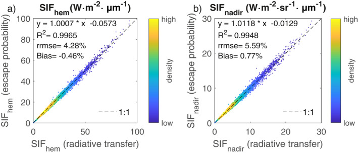
Evaluation of the escape probability method that we have incorporated in the Community Land Model version 5 with the Soil Canopy‐Observation of Photosynthesis and Energy fluxes model for (a) hemispherically integrated solar‐induced chlorophyll fluorescence (SIF) at top‐of‐canopy (TOC) (SIFhem) and (b) TOC SIF at the nadir direction (SIFnadir). Large SIF values not expected to be found in observations are simulated with combinations of extreme input parameter values. Evaluation with a more realistic SIFnadir range of 0–10 W⋅m−2⋅sr−1⋅μm−1 is provided as Figure S3 in Supporting Information S1.
3.2. Evaluation of SIF Simulations
3.2.1. Site Level
SIF simulated by CLM5SP‐exp1 matched those simulated by SCOPE well except at US‐NR1 (R 2 > 0.91, RMSE < 0.19 W⋅m−2⋅sr−1⋅μm−1, Figure 3). Relatively larger deviations were found between simulations by both models and tower observations (RMSE ranged from 0.30 to 0.53 W⋅m−2⋅sr−1⋅μm−1), while the day‐to‐day variation of SIF were generally captured except at US‐NR1 (R 2 ranged from 0.56 to 0.84, Figure 3). The magnitude of satellite SIF was similar to that of tower SIF at Pace Forest, Harvard Forest, and US‐NE3, while much larger day‐to‐day variation was observed for satellite SIF (Figure 3). At the temperate forest sites (Pace Forest and Harvard Forest), SIF simulated by CLM5SP‐exp1 and SCOPE correlated very well and had similar magnitudes (R 2 > 0.98, RMSE < 0.13 W⋅m−2⋅sr−1⋅μm−1, Figures 3a, 3b, 3d and 3f). The models also captured the day‐to‐day variations of SIF observed from the towers at the two sites (R 2 = 0.69 and 0.84 for Pace Forest and Harvard Forest, respectively), while both models overestimated observed SIF (by 0–1.5 W⋅m−2⋅sr−1⋅μm−1, Figures 3a, 3c, 3d and 3f). At the evergreen needleleaf forest site (US‐NR1), SIF simulated by CLM was lower than that simulated by SCOPE, and the correlation between SIF simulated by the two models was lower compared with other sites (R 2 = 0.45, Figures 3g and 3h). This can be explained by the large difference between the optical properties of needleleaves simulated by SCOPE and prescribed in CLM5 and the impact of snow on CLM simulation in winter (see Section 4.1 and Figures S4–S7 in Supporting Information S1). SIF simulated by CLM5SP‐exp1 at US‐NR1 was also higher than SIF observed from tower and satellite and did not fully capture the drop of SIF in winter observed by the tower (R 2 = 0.12, Figures 3g–3i). However, the winter drop of SIF can be captured by CLM5SP‐exp9 with the sustained NPQ formulation by Raczka et al. (2019) (R 2 = 0.57, Figures S8 and S9 in Supporting Information S1). SIF simulated by CLM5SP‐exp1 and SCOPE correlated well at cropland (US‐NE3, R 2 = 0.96, RMSE = 0.13 W⋅m−2⋅sr−1⋅μm−1), and the magnitudes of simulated and observed SIF were similar (Figures 3j–3l). While only moderate correlation was observed between SIF simulated by CLM5SP‐exp1 and observed from tower, this can be partially explained by the relatively smaller variation of SIF magnitude as only data from doy 198–258 was available (Schober et al., 2018). At BR‐Sa1, tower SIF measurement was not available. The magnitude of SIF simulated by CLM5SP‐exp1 and SCOPE matched (R 2 = 0.91, RMSE = 0.18 W⋅m−2⋅sr−1⋅μm−1), while the models overestimated SIF observed by GOME‐2. While the magnitudes of satellite SIF retrievals are generally comparable with tower SIF observations, the correlations between satellite SIF and both tower SIF and simulated SIF were low (R 2 < 0.6), which can be explained by the large pixel size and low single‐observation precision of satellite observations (Joiner et al., 2013).
Figure 3.

Comparisons between nadir solar‐induced chlorophyll fluorescence at 13:30 simulated by the Soil Canopy‐Observation of Photosynthesis and Energy fluxes model (blue solid lines), simulated by CLM5SP‐exp1 (orange dash‐dotted line), observed from the tower (green dashed lines) and observed from satellites (asterisks, corrected to 13:30 for Global Ozone Monitoring Instrument 2) at Pace Forest (a–c), Harvard Forest (d–f), US‐NR1 (g–i), US‐NE3 (j, k, l), and BR‐Sa1 (m and n).
3.2.2. Global Scale
The increase in simulation time was less than 3% when the simulation of SIF was incorporated. Spatial patterns of the multi‐year average SIF (2008–2014) simulated by CLM and observed by GOME‐2 were generally similar, while the magnitude of SIF was different in some regions (Figures 4a, 4c and 4f). CLM simulations and GOME‐2 observations showed the same geographic locations of the SIF hotspots and coldspots (i.e., highest SIF in tropical forests and lower SIF in barren regions). Compared with GOME‐2 SIF, both CLM5SP‐exp1 and CLM5BGC‐exp1 overestimated SIF in boreal (by ∼40%) and tropical (by ∼20%) regions (Figures 4e and 4h) and underestimated SIF in croplands (by 0%–80%). CLM5BGC‐exp1 underestimated SIF in tropical savannas while CLM5SP‐exp1 overestimated SIF.
Figure 4.

Global maps of (a) multi‐year average solar‐induced chlorophyll fluorescence (SIF) from Global Ozone Monitoring Instrument 2 (GOME‐2) product (2008–2014), (b) zonal mean of nadir SIF observed by GOME‐2 (blue solid line), simulated by CLM5SP‐exp1 (orange dash‐dotted line), and simulated by CLM5BGC‐exp1 (green dashed line), (c) multi‐year average nadir SIF simulated by CLM5SP‐exp1 (2008–2014), (d) difference between CLM5SP‐exp1 SIF and GOME‐2 SIF, (e) relative difference between CLM5SP‐exp1 SIF and GOME‐2 SIF, (f) multi‐year average nadir SIF simulated by CLM5BGC‐exp1 (2008–2014), (g) difference between CLM5BGC‐exp1 SIF and GOME‐2 SIF, and (h) relative difference between CLM5BGC‐exp1 SIF and GOME‐2 SIF. In panels e and h, relative differences are calculated as (CLM − GOME)/CLM. In panels d, e, g, and h, pixels with CLM SIF less than 0.1 W⋅m−2⋅sr−1⋅μm−1 are masked in gray.
Both CLM5SP‐exp1 and CLM5BGC‐exp1 SIF simulations correlated well with GOME‐2 SIF at the annual scale (R 2 = 0.8 for CLM5SP‐exp1 and R 2 = 0.7 for CLM5BGC‐exp1, Figure 5). Overall, CLM5SP‐exp1 provided SIF with similar magnitude as observed by GOME‐2 (with a slope of k fit = 1.01 and an intercept of 0.03 W⋅m−2⋅sr−1⋅μm−1 for the fitted line between CLM SIF and GOME‐2 SIF), while CLM5BGC‐exp1 underestimated SIF (with k fit = 0.86 and an intercept of 0.02 W⋅m−2⋅sr−1⋅μm−1). When we excluded some radiative transfer processes or one of the modifications of CLM parameterization (CLM5SP‐exp2‐CLM5SP‐exp6), CLM5SP SIF and GOME‐2 SIF were also highly correlated (R 2 ≥ 0.79, Table 4), but the magnitude of simulated SIF differed (k fit ranged from 0.93 to 1.35. Ignoring the bidirectional effect, canopy clumping, or excluding the correction of PAR (CLM5SP‐exp2‐CLM5SP‐exp4) resulted in SIF 34%, 9%, and 12% higher than that simulated by CLM5SP‐exp1, respectively. The improvements by considering bidirectional effect were most significant in the subtropical grassland region where LAI was lower and leaves were more vertical (Figure S10d in Supporting Information S1), consistent with the expectation that the impact of viewing angle is the largest when LAI is low and leaves are vertical (Biriukova et al., 2020). The improvements by considering clumping index can be seen in most regions where CLM overestimated SIF (Figure S10e in Supporting Information S1). And the impact of the correction of PAR was most significant in tropical forests, where vegetation productivity are radiation limited (Figure S10f in Supporting Information S1; Nemani et al., 2003). Modifications of APAR did not change the simulated APAR substantially in most scenarios, and thus had little impact on the SIF simulations (CLM5SP‐exp5). The modification of leaf and stem optical properties increased simulated SIF by around 7%, and thus increased k fit (CLM5SP‐exp1 as compared with CLM5SP‐exp6). Modification for V cmax had minor impact on SIF simulations (CLM5SP‐exp7, this may not be true if other fluorescence models are used, see Section 4.1). Modeling of NPQ also affected SIF simulation: CLM5SP simulated SIF was 17% lower when K N was adapted to measurements from a drought experiment (CLM5SP‐exp8) than when K N was adapted to a cotton data set with measurements with varying light, temperature, and CO2 conditions (CLM5SP‐exp1). The multi‐year mean SIF simulated by CLM5SP‐exp1 correlated well with those observed by OCO‐2 and TROPOMI (R 2 = 0.84 for OCO‐2 and R 2 = 0.82 for TROPOMI), even though model simulations and satellite products cover different periods of time (CLM: 2008–2014, OCO‐2: September 2014 to April 2018, TROPOMI: April 2018 to March 2020). SIF simulated by CLM was generally lower compared with OCO‐2 observations while provided similar magnitude as TROPOMI observations (with k fit of 0.85 and 0.95, respectively, and intercepts of around 0.05 W⋅m−2⋅sr−1⋅μm−1, Table 4).
Figure 5.

Scatter plots between multi‐year average (2008–2014) Global Ozone Monitoring Instrument 2 (GOME‐2) solar‐induced chlorophyll fluorescence (SIF) and (a) CLM5SP‐exp1 SIF (b) CLM5BGC‐exp1 SIF. Pixels dominated (>70% land unit) by several plant functional types (PFTs) are colored according to the legend. Gray dots indicate pixels not dominated by any listed PFTs. The means and standard deviations of CLM5SP SIF and GOME‐2 SIF for each PFT are shown as squares and error bars, respectively.
Table 4.
Statistics for Comparisons Between SIF Simulated by CLM and Observed by Satellites
| Simulation | Satellite | Slope (k fit) | Intercept (W⋅m−2⋅sr−1⋅μm−1) | R 2 | RMSE (W⋅m−2⋅sr−1⋅μm−1) |
|---|---|---|---|---|---|
| CLM5SP‐exp1 | GOME‐2 | 1.01 | 0.03 | 0.80 | 0.0661 |
| CLM5SP‐exp2 | 1.35 | 0.04 | 0.82 | 0.0843 | |
| CLM5SP‐exp3 | 1.11 | 0.04 | 0.80 | 0.0723 | |
| CLM5SP‐exp4 | 1.17 | 0.03 | 0.80 | 0.0765 | |
| CLM5SP‐exp5 | 0.99 | 0.03 | 0.79 | 0.0671 | |
| CLM5SP‐exp6 | 0.93 | 0.03 | 0.79 | 0.0624 | |
| CLM5SP‐exp7 | 1.02 | 0.03 | 0.80 | 0.0665 | |
| CLM5SP‐exp8 | 0.84 | 0.03 | 0.82 | 0.0521 | |
| CLM5BGC‐exp1 | 0.86 | 0.02 | 0.70 | 0.0747 | |
| CLM5SP‐exp1 | OCO‐2 | 0.85 | 0.05 | 0.84 | 0.0582 |
| CLM5SP‐exp1 | TROPOMI | 0.95 | 0.05 | 0.82 | 0.0639 |
Note. SIF, solar‐induced chlorophyll fluorescence; CLM, Community Land Model.
The relationships between SIF simulated by CLM and observed by satellites were different depending on the PFT. While seasonal variations of SIF were captured by CLM for most PFTs, the magnitude of SIF was not accurately simulated for some PFTs (Figure 6). Both CLM5SP‐exp1 and CLM5BGC‐exp1 underestimated peak growing season SIF for broadleaf deciduous temperate tree (by ∼20%), overestimated SIF for tropical tree (by ∼30%), underestimated SIF for crop during the growing season (by ∼40%), and estimated SIF relatively accurate for C3 non‐arctic grass (Figures 5 and 6). For needleleaf evergreen boreal tree, CLM5SP‐exp1 overestimated SIF throughout the year, while CLM5BGC‐exp1 overestimated SIF during boreal winter and underestimated SIF during the growing season. Trends of seasonal variations were similar when CLM SIF was compared with OCO‐2 SIF and TROPOMI SIF (see Figures S11 and S12 in Supporting Information S1).
Figure 6.

Comparison between seasonal variations (average of 2008–2014) of solar‐induced chlorophyll fluorescence observed by Global Ozone Monitoring Instrument 2 (blue solid lines), simulated by CLM5SP‐exp1 (orange dashed lines), and simulated by CLM5BGC (green dash‐dotted lines) for (a) broadleaf deciduous temperate tree, (b) needleleaf evergreen boreal tree, (c) broadleaf evergreen tropical tree, (d) crop, and (e) C3 non‐arctic grass. All pixels dominated (>70% land unit) by the corresponding plant functional type were used for comparison, locations of the pixels are the same for CLM5SP and CLM5BGC and are shown in panel (f): blue: broadleaf deciduous temperate tree, cyan: needleleaf evergreen boreal tree, green: broadleaf evergreen tropical tree, yellow: crop, and red: C3 non‐arctic grass.
4. Discussions
This study incorporates simulation of nadir SIF at 740 nm into CLM5 with improved representation of radiative transfer (Table 1). The strong agreement between simulations by SCOPE and CLM (except in needleleaf forest) indicates that the key radiative transfer processes were properly taken into account, despite using a more efficient approach based on escape probability instead of the full radiative transfer scheme to scale leaf‐level SIF to observed canopy‐level SIF. While CLM simulations generally captured the spatial and seasonal variations of observed SIF, discrepancies between simulations and observations were observed for some sites and PFTs, suggesting uncertainties in model simulations, which will be discussed in the following sections. By providing better representation of the radiative transfer of SIF, our work is a step toward better SIF simulation by LSMs and the use of satellite SIF observations for constraining or evaluating GPP simulations.
4.1. Impacts of Key Radiative Transfer Processes and Model Parameterizations on SIF Simulation
Compared with previous works that incorporate simulation of SIF into LSMs (Table 1), our model provides a mechanistic way to scale SIF from leaf‐level to TOC at the nadir direction by taking into account canopy scattering, the bidirectional effect, corrections for PAR and APAR, and canopy clumping (Sections 2.1.2, 2.1.3, 2.1.4, 2.1.5). We also updated some model parameterizations (leaf optical properties and V cmax) according to recent data sets. Some of the processes and parameterizations (bidirectional effect, canopy clumping, incident PAR, plant optical properties, and parameterizations of photosystem‐level fluorescence model) have significant impacts on SIF simulations, and need to be properly taken into account.
When the bidirectional anisotropic effect is not considered, SIF radiance observed by sensor is usually estimated as SIFhem/π by assuming isotropic SIF signal at TOC. However, model simulations, field measurements, and satellite observations have shown that observed SIF varies with viewing angle (Biriukova et al., 2020; Liu et al., 2016; Zeng et al., 2020; Zhang et al., 2018; Zhao et al., 2016): SIF is usually lower when observed at small VZA and higher when observed at large VZA, indicating that nadir SIF is usually lower than SIFhem/π. Consistent with these studies, our simulations showed that not considering the bidirectional effect resulted in an increase of simulated nadir SIF by 34%. The hot spot effect also affects the variation of SIF with viewing angle. This effect is not considered in this study for simplicity. Our CLM simulations were compared with satellite observations by filtering out observations at small phase angles (Section 2.2). However, if satellite observations with small phase angles are used, the impact of hot spot might need to be taken into account.
While natural vegetation canopies are heterogeneous (in terms of leaf and stem distribution), most LSMs assume canopy structure to be homogeneous due to limited computational capacity and the lack of 3D canopy structure data. However, the 3D distribution of plant materials affects observed SIF by affecting both incident PAR on leaves and the radiative transfer of SIF toward the sensor. Studies have suggested significant differences between SIF simulated with a homogeneous canopy scene and a heterogeneous scene with 3D canopy structure when other canopy properties were kept identical (Hernández‐Clemente et al., 2017; Zeng et al., 2020; Zhao et al., 2016). The heterogeneity of canopy can be partially characterized by clumping index in analytical radiative transfer models (J. M. Chen et al., 1991). We introduced a simple PFT‐specific clumping index in CLM5, which resulted in lower SIF values compared with when clumping was not considered (∼9% at the global scale, CLM5SP‐exp1 compared with CLM5SP‐exp3, Table 4). It should also be noted that the PFT‐specific clumping index cannot fully characterize the heterogeneity of canopy. For instance, studies have shown that clumping index varies with SZA, and considering this angular dependency may improve the simulation of photosynthesis (Braghiere et al., 2020; Ryu et al., 2010).
Incident PAR is one of the key drivers of SIF. When not coupled with the CAM, the original CLM estimates incident PAR by assuming a fixed ratio of 0.5 between incident PAR and shortwave radiation (CLM5.0 Technical Description, 2020). However, the ratio (0.5) is too high according to literature, especially when PAR is defined as 400–700 nm as in CLM (Tsubo & Walker, 2005). Based on measurements at 31 AmeriFlux sites (Table S1 in Supporting Information S1), we set the ratio between incident PAR and shortwave radiation to 0.435 for simulation of photosynthesis and fluorescence (except CLM5SP‐exp4). This correction had a notable impact (16% decrease, Table 4) on simulated SIF. We also note that the ratio we used was derived from measurements from flux towers across the Americas only, and the ratio varies spatially and temporally (Tsubo & Walker, 2005). More comprehensive observation data set or simulations based on atmospheric radiative transfer is needed to provide more accurate incident PAR for CLM. If CLM is coupled with the CAM, this correction we made would not be needed as CAM would provide incident PAR simulated based on radiative transfer as input for CLM.
We made two modifications to the calculation of APAR in CLM (except for CLM5SP‐exp5). (a) We used PAR absorbed by leaf only for simulation of photosynthesis while the original CLM5 uses PAR absorbed per unit plant (leaf and stem) area to approximate PAR absorbed per leaf area. As leaf absorption is higher than stem absorption in the visible region, APAR per unit leaf area is slightly greater than APAR per unit plant area. Therefore, distinguishing PAR absorbed by leaf and by stem leads to greater APAR and thus an overall slight increase in simulated SIF (k fit increased from 0.99 to 1.01, Table 4). Note that the relatively small impact of this modification on SIF simulation is due to the small impact of the modification on APAR simulation itself, and this does not indicate SIF simulation is not sensitive to APAR. (b) We excluded PAR absorbed by snow in the calculation of photosynthesis and SIF. Due to the lower APAR, simulated SIF was lower in boreal winter compared to SIF simulated without the modification (25% and 0.06 W⋅m−2⋅sr−1⋅μm−1 in CLM5SP for needleleaf evergreen deciduous tree, Figure S14 in Supporting Information S1). Stem and snow are not present in SCOPE. The absence of stem may also explain the higher APAR and escape probability simulated by SCOPE compared with that by CLM (5%–15% at sites except for US‐NR1 in the growing season, Figures S4 and S6 in Supporting Information S1). And, snow explains the fluctuation of escape probability and nadir reflectance simulated by CLM for US‐NR1 (Figures S6 and S7 in Supporting Information S1).
Leaf and stem optical properties affect the radiation absorbed and scattered by the canopy, and thus affect the simulation of GPP and SIF. However, the leaf and stem optical properties used in the original CLM are from data sets produced in the 1990s or earlier (Asner et al., 1998; Majasalmi & Bright, 2019; Sellers et al., 1986). Recently, Majasalmi and Bright (2019) revisited the values used by CLM5. They found that the optical properties in the visible band in the original CLM5 fell within the range of measured values, but those in the NIR bands were notably different from measured values. Measured leaf single scattering albedo (the sum of reflectance and transmittance) was more than 60% larger than CLM default values for conifer PFTs and more than 10% larger for broadleaf PFTs (Majasalmi & Bright, 2019). Using leaf and stem optical properties provided by Majasalmi and Bright (2019) instead of the default values induced notable difference in simulated SIF (k fit increased from 0.93 to 1.01, Table 4). Besides, the PROSPECT model (Féret et al., 2017) used by SCOPE is more suitable for simulating leaf optical properties for broad leaves than for needles. In addition to the absence of stem in SCOPE, the difference between leaf optical properties simulated by SCOPE and that in CLM contributed to the large difference (around 35% in the growing season) in APAR and SIF simulated by the two models for the needleleaf US‐NR1 site. With the availability of hyperspectral data from airborne and satellite missions (e.g., AVIRIS‐NG, Surface Biology and Geology, and EnMap), the plant optical properties in future generations of models could be constrained by observed canopy reflectance.
Sensitivity analyses with SCOPE have shown that the sensitivity of simulated SIF to V cmax is different when different models are used to simulate fluorescence yield (Verrelst et al., 2015). Variations in V cmax contributed less than 2% variability of simulated SIF for the model we used (except for CLM5SP‐exp8), while contributed around 10% variability for three other models (Verrelst et al., 2015). This difference can be mainly attributed to the difference in the calculation of K N in these models and is further discussed in Section 4.2. Consistent with Verrelst et al. (2015), we only found a minor impact (less than 1.5% impact on fitted line between CLM5SP SIF and GOME‐2 SIF) of changing the default PFT‐specific V cmax values in CLM to those provided by Bonan et al. (2011) on SIF simulation (Table 4).
4.2. Uncertainties in SIF Simulations
We have shown that SIF simulated by CLM5SP‐exp1 agreed well with SIF simulated by the widely used SCOPE model at sites except for US‐NR1, but some discrepancies where found between model simulations and observations at both site‐level and the global scale. Below we discuss the sources of uncertainty in SIF simulations.
First of all, the choice of fluorescence emission model has large impact on SIF simulation. Multiple models have been developed to simulate fluorescence yield at the photosystem‐level (Bennett et al., 2018; Johnson & Berry, 2021; Lee et al., 2013; Porcar‐Castell, 2011; van der Tol et al., 2014; Zaks et al., 2012). Most models focus on photosystem II or do not distinguish fluorescence emission from the two photosystems due to the lack of available data (Porcar‐Castell et al., 2021; van der Tol et al., 2014). However, the distribution of fluorescence emission from the two photosystems is one of the challenges for interpreting and accurate simulating fluorescence emission (Porcar‐Castell et al., 2021). Another source of uncertainty is from the modeling of NPQ (e.g., Equations 5d and 8 in Section 2.1.1), which is also the major difference between the models. NPQ is typically related to relative light saturation and the level of environmental stress. Various empirical relationships have been built based on measurements with different species and environmental settings (Lee et al., 2013; van der Tol et al., 2014). We found that the magnitude of CLM5SP simulated SIF was 17% smaller when K N was adapted to the drought data set (CLM5SP‐exp8) compared with when it was adapted to the cotton data set (CLM5SP‐exp1). Some models further take into account slower changes in NPQ (sustained NPQ), which is important for temporal and boreal evergreen species (Raczka et al., 2019). Studies at US‐NR1 have shown notable impact of the modeling of sustained NPQ on SIF simulated by LSMs for evergreen needleleaf forest (Parazoo et al., 2020; Raczka et al., 2019). At US‐NR1, SIF simulated with the sustained NPQ formulation (CLM5SP‐exp9) captured the seasonal day‐to‐day variation of tower SIF observation better than CLM5SP‐exp1 (R 2 = 0.57, compared with R 2 = 0.12, Figure 3 and Figure S9 in Supporting Information S1). However, it is challenging to apply the models with sustained NPQ to larger scales as they rely on calibration with experimental data sets (Porcar‐Castell, 2011; Raczka et al., 2019) and it is uncertain how the parameters vary spatially. As all the photosystem‐level fluorescence models were calibrated with limited measurements on only a handful of species, it is uncertain which model is more appropriate for global‐scale simulations. Thus, there is a need for a more comprehensive data set of leaf‐level measurements that covers various PFTs and different environmental conditions (Helm et al., 2020; Magney et al., 2017).
Another major source of uncertainty in SIF simulation is the fluorescence quantum efficiency (FQE) in models, which is linearly correlated with the absolute SIF value (Vilfan et al., 2016). A fixed FQE (i.e., the default value of 0.01) is usually used in SIF simulations. But studies have shown that using the fixed value can lead to systematic deviation in simulated SIF, and there can be a seasonal variation in FQE (Hu et al., 2018). So far, there are very few observational constraints on the magnitude and seasonal variations of FQE. Besides, there is uncertainty associated with the leaf‐level fluorescence yield under dark‐adapted condition . In the SCOPE model, is determined by leaf biochemical and biophysical parameters (e.g., leaf pigment content, water content, dry matter content, and leaf structure), FQE, and the spectral distribution function for fluorescence emission (Vilfan et al., 2016). Due to the absence of these parameters in CLM, we obtained an empirical using the LOPEX93 data set and SCOPE simulations (Section 2.1.1). As there is limited observations of , it is uncertain whether the value is representative for various biomes. simulated by default SCOPE input is also lower than the value we used for CLM simulations due to the deviation of leaf dry matter content in the LOPEX93 data set from the default value in SCOPE, contributing to the difference between Φ f simulated by CLM and SCOPE (Figure S5 in Supporting Information S1).
In this study, the new spectral distribution of fluorescence emission calibrated with measurements from soybean leaves was used for SCOPE simulations and deriving as recommended by SCOPE v1.73 (van der Tol et al., 2019). This new spectral distribution function simulates SIF with spectral shape more in line with measurements from soybean leaves and does not distinguish the two photosystems as the previous versions do (van der Tol et al., 2019). However, the change in spectral distribution also leads to around 30% higher than that simulated based on the previous version of spectral distribution function (Figure S13 in Supporting Information S1), and the magnitude of SIF simulation based on the new spectral shape has not been well evaluated (van der Tol et al., 2019). When the previous version of spectral distribution function was used, simulated SIF was more in line with tower observations compared with when the new version of spectral distribution function was used except at US‐NE3 (Figure S13 in Supporting Information S1). For instance, simulated SIF was around 0.5 W⋅m−2⋅sr−1⋅μm−1 higher than tower observation at Pace Forest in peak growing season when the old spectral distribution function was used, while around 1.2 W⋅m−2⋅sr−1⋅μm−1 higher when the new version was used (Figure S13 in Supporting Information S1). More observations are needed to evaluate the FQE value and the spectral distribution of SIF emission.
Besides, LSMs cannot accurately represent all processes, and model parameterizations can be inaccurate. Thus, it is not expected that CLM SIF would perfectly match observed SIF even when the simulation of fluorescence yield and the observation of SIF is accurate. As biases are found in CLM5 GPP simulations (Lawrence et al., 2019), simulations of SIF, which is closely linked to GPP, can also be biased. On the other hand, models can get simulations close to observations for the wrong reason. Biases in SIF simulations are not necessarily bad as they open up windows for improving the models and using satellite observations to constrain model simulations of SIF and GPP. As discussed in Section 4.4, inaccurate model parameterizations (e.g., LAI and leaf angle distribution) likely caused some biases in SIF simulation. The lower correlation between CLM5BGC SIF and GOME‐2 SIF compared with the correlation between CLM5SP SIF and GOME‐2 SIF (Table 4) may also indicate that the larger uncertainty in the fully prognostic CLM5BGC (e.g., in simulation of LAI) could lead to larger uncertainty in SIF simulation. The accuracy of the land cover data prescribed for CLM5SP or simulated by CLM5BGC can also affect SIF simulation. Besides, there is no seasonal or interannual variation of leaf optical properties and leaf angle distribution in CLM5SP and CLM5BGC and no interannual variation of LAI in CLM5SP, which may introduce errors in SIF simulation. Ground‐based measurements of the seasonality of leaf optical properties are needed but have rarely been collected (X. Yang et al., 2016). Future satellite observations from the Surface Biology and Geology mission can provide canopy spectra at a temporal resolution of around 16 days and may be used for parameterization in models. Furthermore, a more complex canopy representation can improve model performance. Considering a multilayer canopy as opposed to a one‐layer canopy with sunlit and shaded leaves (as used by CLM5) has been shown to improve the simulation of canopy fluxes (Bonan et al., 2018, 2021; Wang & Frankenberg, 2021). And, simpler canopy representations in models can overestimate SIF according to simulations by P. Yang, Verhoef, and van der Tol (2017) and Wang and Frankenberg (2021).
4.3. Uncertainties in Satellite SIF Products
Uncertainties in satellite SIF products should also be taken into account when comparing model simulated SIF and satellite SIF products. While multiple SIF products have been produced with measurements from different satellites, substantial discrepancies across products have been observed (Parazoo et al., 2019). The discrepancies can be attributed to differences in sensor characteristics and retrieval algorithms (Parazoo et al., 2019). For instance, OCO‐2 and GOSAT SIF are higher compared with GOME‐2 SIF in the pan‐tropics (Sun et al., 2018), and GOME‐2 SIF produced with different retrieval algorithms reveals a difference in magnitude of up to a factor of 2 (Parazoo et al., 2019). Our results also showed different biases in CLM5SP‐exp1 SIF when compared with different SIF products (Table 4). CLM5SP‐exp1 SIF agreed better with GOME‐2 SIF and TROPOMI SIF than with OCO‐2 SIF in terms of magnitude (note that OCO‐2 SIF and TROPOMI SIF were from different years compared with CLM SIF). Another uncertainty associated with OCO‐2 SIF is that the original OCO‐2 product is SIF retrieved at 757 nm and it was converted to 740 nm with a factor of 1.56 according to Köhler et al. (2018) for the comparison with CLM SIF. However, while multiple studies have made conversions between satellite observed SIF at 757 nm and at 740 nm, there is no consensus on the conversion factor: the ratio between SIF at 740 nm and at 757 nm used ranges from 1.50 to 1.69 (Köhler et al., 2018; Parazoo et al., 2019; Sun et al., 2018). Moreover, while satellite products are TOC SIF, most of these conversion factors were derived from leaf‐level measurements and thus do not account for the canopy‐scale scattering and reabsorption. Considering that reabsorption is stronger at 740 nm than at 757 nm, the conversion factor at the canopy scale may be lower than the reported leaf‐level factors. The conversion factor may also vary spatially and temporally due to variations of canopy structure and leaf biochemical and biophysical properties. The illumination conditions for CLM simulations and satellite observations are also not identical, as all satellite SIF products applied cloud filtering while no filter was applied to CLM simulations based on illumination conditions (Zhang et al., 2020). This can contribute to discrepancies between simulated and observed SIF and lead to clear‐sky bias when linking satellite SIF observation with GPP. Filtering simulations based on cloud condition may improve the comparison between simulations and observations and the assimilation of observed SIF. And, the clear‐sky bias can be mitigated by applying corrections to SIF simulations (Hu et al., 2021; Zhang et al., 2020). The spatial resolutions are also different between the satellite SIF products and CLM simulations, and may affect the simulation‐observation comparisons.
4.4. Analysis for Different PFTs
The agreement between SIF simulations and observations varied depending on the PFT and the types of models and observations. At sites where tower SIF was measured from broadleaf deciduous temperate tree (Pace Forest and Harvard Forest), SIF simulated by CLM5SP‐exp1 generally matched that simulated by SCOPE (R 2 > 0.98, RMSE < 0.13 W⋅m−2⋅sr−1⋅μm−1, Figures 3a–3f). However, the models overestimated SIF at site level compared with tower and satellite observations, while CLM5SP‐exp1 slightly underestimated SIF for broadleaf deciduous temperate tree at the global scale (Figures 3a, 3d and 6). Further investigation is needed to determine the cause of the discrepancies between simulated and observed SIF. Some potential factors include: the discrepancy between the footprints of the tower‐based observations and CLM, resulting in a wide range of mismatch (e.g., MODIS LAI and LAI in the field of view of SIF sensor at the towers); uncertainties in fluorescence emission model (as described in Section 4.2); the lack of seasonality in leaf optical properties in the models; and the absence of some key parameters affecting SIF simulations such as chlorophyll content in CLM (Verrelst et al., 2015). Besides the above‐mentioned factors, the different performance of simulation at the sites and at the global scale might relate to the different locations of the sites and the pixels used for global‐scale analysis: while there was only deciduous trees in the field of view of the SIF sensors, the sites locate in mixed forests; however, only 11 pixels dominated by broadleaf deciduous temperate tree were used for the global‐scale analysis (Figure 6).
At the subalpine needleleaf evergreen forest site (US‐NR1), SIF simulated by CLM5SP‐exp1 was lower than that simulated by SCOPE while higher than that observed at the tower (Figures 3g–3i), which is consistent with previous studies at the site (Parazoo et al., 2020; Raczka et al., 2019). As discussed in Parazoo et al. (2020) and Raczka et al. (2019), various factors related to models and observations can lead to the discrepancy. Specifically, the smaller seasonal variation of simulated SIF compared with observed SIF can possibly be explained by the absence of sustained NPQ in the fluorescence model. With sustained NPQ incorporated into CLM5SP according to Raczka et al. (2019), CLM5SP‐exp9 captured the day‐to‐day variation of tower‐observed SIF throughout the year (R 2 = 0.57; Figures S8 and S9 in Supporting Information S1). At the global scale, CLM5SP‐exp1 consistently overestimated SIF throughout the year for needleleaf evergreen boreal tree, while CLM5BGC‐exp1 simulated similar multi‐year average SIF as observed by GOME‐2 but with smaller seasonal variation (Figure 6b). The large difference between SIF simulated by CLM5SP‐exp1 and CLM5BGC‐exp1 can be attributed to the difference between prescribed LAI used by CLM5SP and prognostic LAI simulated by CLM5BGC, neither of which captured the magnitude and seasonal variation of MODIS LAI (Figure S15a in Supporting Information S1). The smaller seasonal variation of SIF simulated by CLM5BGC can also possibly be explained by the absence of sustained NPQ in the fluorescence model (Raczka et al., 2019).
CLM simulations underestimated SIF in cropland during the peak growing season at both site‐level and the global scale (Figures 3j and 6d). While both CLM5SP‐exp1 and CLM5BGC‐exp1 underestimated SIF, the reasons for the underestimation may be different. CLM5SP uses prescribed LAI and does not account for any management or crop‐specific phenology and allocation. The underestimation of CLM5SP SIF might have resulted from inaccurate parameterizations of LAI and LAD for crop. The peak growing season LAI used by CLM5SP for cropland in the United States was below 2.5 m2⋅m−2 and relatively close to MODIS LAI (Figure S15b in Supporting Information S1). However, it has been shown that the peak growing season LAI should be around 5 m2⋅m−2 in the U.S. corn belt and that traditional LAI products (e.g., MODIS LAI) significantly underestimated LAI in this region (Kimm et al., 2020). For US‐NE3, the peak LAI value from MODIS is 3 m2⋅m−2, while field measurements showed a peak LAI around 4 m2⋅m−2 (Peng et al., 2018). Besides, the mean leaf zenith angle for crop was set to 70° in CLM5SP, which might be too vertically oriented (Ku et al., 2010; Rosa & Forseth, 1996; Ross, 1981). In the global scale CLM5SP‐exp1 simulation, all crop was assumed to be C3 as default, which can also lead to inaccurate simulations. For simulation at US‐NE3, the photosynthetic pathway was set to be C4 for maize. For CLM5BGC, explicit crop types and management are considered, and LAI is prognostic. LAI simulated by CLM5BGC was higher than that from CLM5SP and MODIS (with a peak growing season value of 4.4 m2⋅m−2, Figure S15 in Supporting Information S1), and may be closer to the truth. The underestimation of SIF by CLM5BGC may result from the LAD assigned to the relevant crop functional types. For both maize and soybean, the two major crop functional types in the U.S., mean leaf zenith angles were assigned to be 75°, which indicates even more vertical leaves than those in default CLM5SP. Using more realistic LAD would likely bring CLM5BGC SIF closer to observed values.
CLM5SIF‐exp1 simulation generally matched SCOPE simulation at the tropical evergreen forest site BR‐Sa1 (R 2 > 0.91, RMSE < 0.19 W⋅m−2⋅sr−1⋅μm−1, Figures 3m and 3n), but both models simulated higher SIF compared with GOME‐2 observation (Figure 3m). Simulations of SIF by CLM5SP‐exp1 and CLM5BGC‐exp1 were similar for broadleaf evergreen tropical tree throughout the year, and both overestimated SIF as compared with GOME‐2 observations (Figure 6c). Previous studies have noted the challenges of accurately simulating biological processes in tropical regions in LSMs (Christoffersen et al., 2014; Wu et al., 2016). Besides, one study found that OCO‐2 and GOSAT SIF products had higher values in the pan‐tropics compared with GOME‐2 SIF (Sun et al., 2018), highlighting that the satellite estimates of SIF also vary in this region. CLM5SP SIF compared better with OCO‐2 SIF in the tropics (relative error ∼10% in Figure S11 in Supporting Information S1 as opposed to ∼30% in Figure 6c).
4.5. Limitations and Future Directions
Besides improvements in CLM parameterizations (e.g., for LAI and leaf angle distribution), CLM SIF simulation may be improved by: (a) improving the simulation of photosystem‐level fluorescence yield, especially the modeling of NPQ, based on more advanced models and/or more comprehensive calibration data sets; (b) considering the variation of dark‐adapted leaf‐level fluorescence yield with PFT and season; (c) incorporating SIF simulation for arbitrary viewing direction so that model simulations can be compared with measurements from different viewing angles (e.g., measurements from the OCO‐2 glint mode and the edge of swath of GOME‐2 and TROPOMI measurements); (d) adding an additional band (740 nm or 757 nm) in the model for SIF simulation, thus eliminating the impact of the difference between leaf optical properties at the certain wavelength and at the NIR band on simulation of SIF radiative transfer. In addition, further investigation on the response of SIF and GPP to stress and more evaluation of SIF simulations with tower‐based SIF observations are needed (H. Yang, Yang, et al., 2017; X. Yang et al., 2018; Magney, Bowling, et al., 2019; Miao et al., 2018; Helm et al., 2020; Marrs et al., 2020).
A potential of the model we developed is to constrain the simulation of photosynthesis in LSMs by assimilating satellite SIF observations. As the response of SIF and GPP to stress may be different (He et al., 2020; Helm et al., 2020; Marrs et al., 2020) and there is uncertainty in the fluorescence yield model, there may be cases where biases in GPP simulation do not lead to biases in SIF simulation, and vice versa. Thus, caution needs to be taken when assuming SIF‐GPP relationship at small spatial and temporal scales. However, robust linear relationships between SIF and GPP has been found at larger spatial and temporal scales (Lee et al., 2013; Li et al., 2018; Miao et al., 2018; Magney, Bowling, et al., 2019; Magney et al., 2020; X. Yang et al., 2015). Several studies have demonstrated the potential of constraining GPP simulation with satellite SIF observations: MacBean et al. (2018) assumed a biome‐specific linear relationship between SIF and GPP and showed that model estimation of global GPP became more in line with flux tower‐based GPP when satellite SIF was used to constrain the model. Norton et al. (2018) conducted an error propagation study and showed that parametric uncertainty in modeled global annual GPP could be reduced by 73% from ±19.0 PgC⋅yr−1to ±5.2 PgC⋅yr−1 with data assimilation. Bacour et al. (2019) assimilated OCO‐2 SIF product to constrain ORCHIDEE, and found that the optimized GPP budget agreed well with independent flux tower‐based GPP products. Our model will further enhance the capability to use satellite SIF observations to constrain the simulation of GPP, as simulated and observed SIF can be better compared with a more mechanistic method applied to upscale leaf‐level SIF to TOC nadir SIF. It is also expected that GPP simulations can be better constrained by using both SIF and other remote sensing products, such as LAI, fraction of absorbed PAR, NIRv, and f esc. Recently, advances have been made in harmonizing SIF products from multiple satellites and generating long‐term, high spatial‐resolution global SIF products (Li & Xiao, 2019; Parazoo et al., 2019; Wen et al., 2020). These products may also benefit the potential application of our model on the evaluation of GPP simulation and on data assimilation.
5. Conclusions
We developed a scheme to incorporate the simulation of TOC nadir SIF at 740 nm into CLM5. Compared with previous modeling approaches, our approach takes canopy clumping and key radiative transfer processes into account and enables more robust comparison between simulated and satellite‐observed SIF. SIF simulated by CLM5 agreed well with SIF simulated by the SCOPE model at the temperate forest, cropland, and tropical forest sites, and generally captured the spatial and seasonal patterns of satellite observed SIF. PFT‐dependent discrepancies where found between the magnitudes of simulated and observed SIF at both site‐level and the global scale, which may associate with inaccurate parameterizations of the fluorescence emission model and canopy properties. Our findings suggested that the fluorescence emission model, canopy clumping, the bidirectional effect, and model parameterizations (leaf optical properties, LAI, leaf angle distribution) can significantly affect SIF simulation and should thus be properly taken into account. By providing improved representation of radiative transfer for SIF simulation, our model provides LSM SIF simulation that can be better compared with satellite observations, and can serve as an important step toward the use of satellite SIF observations for constraining and evaluating GPP modeling.
Supporting information
Supporting Information S1
Acknowledgments
The authors thank the editor and the two anonymous reviewers for their constructive comments on the manuscript. X. Yang was funded by the National Aeronautics and Space Administration (80NSSC17K0110), the National Science Foundation through Division of Integrative Organismal Systems (2005574), the Office of Polar Programs (2023205), and the Center for Innovative Technology through Commonwealth Research Commercialization Fund (MF20‐008‐US). M. Shi was partly supported by the U.S. Department of Energy Office of Science Biological and Environmental Research as part of the Terrestrial Ecosystem Science Program through the Next‐Generation Ecosystem Experiments (NGEE) Tropics project. PNNL is operated by the Battelle Memorial Institute for the U.S. DOE under contract DE‐AC05‐76RLO1830. The CESM project is supported primarily by the National Science Foundation (NSF). This material is based upon work supported by the National Center for Atmospheric Research, which is a major facility sponsored by the NSF under Cooperative Agreement 1852977. Computing and data storage resources, including the Cheyenne supercomputer (https://doi.org/10.5065/D6RX99HX), were provided by the Computational and Information Systems Laboratory (CISL) at the NCAR. A portion of this research was carried out at the Jet Propulsion Laboratory, California Institute of Technology, under contract with the NASA. Support from the NASA Earth Science Division Terrestrial Ecology program's Arctic Boreal Vulnerability Experiment (ABoVE) is acknowledged. Operation of the US‐Ha1 site is supported by the AmeriFlux Management Project with funding by the U.S. Department of Energy's Office of Science under Contract No. DE‐AC02‐05CH11231, and additionally is a part of the Harvard Forest LTER site supported by the National Science Foundation (DEB‐1832210). Funding for the AmeriFlux core site US‐NR1 data was provided by the U.S. Department of Energy's Office of Science. The US‐Ne3 AmeriFlux site is supported by the Lawrence Berkeley National Lab AmeriFlux Data Management Program and the Carbon Sequestration Program, University of Nebraska‐Lincoln Agricultural Research Division. Funding for AmeriFlux core site data was provided by the U.S. Department of Energy's Office of Science.
Li, R. , Lombardozzi, D. , Shi, M. , Frankenberg, C. , Parazoo, N. C. , Köhler, P. , et al. (2022). Representation of leaf‐to‐canopy radiative transfer processes improves simulation of far‐red solar‐induced chlorophyll fluorescence in the Community Land Model version 5. Journal of Advances in Modeling Earth Systems, 14, e2021MS002747. 10.1029/2021MS002747
Contributor Information
Rong Li, Email: rl9pzb@virginia.edu.
Xi Yang, Email: xiyang@virginia.edu.
Data Availability Statement
Code and results for CLM5 SIF simulations are available at https://doi.org/10.5281/zenodo.6301355. GOME‐2 SIF data is available at https://avdc.gsfc.nasa.gov/pub/data/satellite/MetOp/GOME_F/; TROPOMI and OCO‐2 SIF data are available at ftp://fluo.gps.caltech.edu/data. SIF observation at Harvard forest is available at https://doi.org/10.6073/pasta/99c883ee28987ac32a98d621c7ec3bb6. SIF observation at US‐NR1 is available at https://doi.org/10.22002/D1.1231. SIF observation at US‐NE3 is available at https://doi.org/10.13012/B2IDB-5893373_V1.
References
- Anav, A. , Friedlingstein, P. , Beer, C. , Ciais, P. , Harper, A. , Jones, C. , et al. (2015). Spatiotemporal patterns of terrestrial gross primary production: A review. Reviews of Geophysics, 53(3), 785–818. 10.1002/2015RG000483 [DOI] [Google Scholar]
- Asner, G. P. , Wessman, C. A. , Schimel, D. S. , & Archer, S. (1998). Variability in leaf and litter optical properties: Implications for BRDF model inversions using AVHRR, MODIS, and MISR. Remote Sensing of Environment, 63(3), 243–257. 10.1016/S0034-4257(97)00138-7 [DOI] [Google Scholar]
- Bacour, C. , Maignan, F. , MacBean, N. , Porcar‐Castell, A. , Flexas, J. , Frankenberg, C. , et al. (2019). Improving estimates of gross primary productivity by assimilating solar‐induced fluorescence satellite retrievals in a terrestrial biosphere model using a process‐based SIF model. Journal of Geophysical Research: Biogeosciences, 124(11), 3281–3306. 10.1029/2019JG005040 [DOI] [Google Scholar]
- Badgley, G. , Field, C. B. , & Berry, J. A. (2017). Canopy near‐infrared reflectance and terrestrial photosynthesis. Science Advances, 3(3), e1602244. 10.1126/sciadv.1602244 [DOI] [PMC free article] [PubMed] [Google Scholar]
- Bennett, D. I. G. , Fleming, G. R. , & Amarnath, K. (2018). Energy‐dependent quenching adjusts the excitation diffusion length to regulate photosynthetic light harvesting. Proceedings of the National Academy of Sciences, 115(41), E9523–E9531. 10.1073/pnas.1806597115 [DOI] [PMC free article] [PubMed] [Google Scholar]
- Berry, J. A. (2012). There ought to be an equation for that. Annual Review of Plant Biology, 63(1), 1–17. 10.1146/annurev-arplant-042811-105547 [DOI] [PubMed] [Google Scholar]
- Biriukova, K. , Celesti, M. , Evdokimov, A. , Pacheco‐Labrador, J. , Julitta, T. , Migliavacca, M. , et al. (2020). Effects of varying solar‐view geometry and canopy structure on solar‐induced chlorophyll fluorescence and PRI. International Journal of Applied Earth Observation and Geoinformation, 89, 102069. 10.1016/j.jag.2020.102069 [DOI] [Google Scholar]
- Blanken, P. D. , Monson, R. K. , Burns, S. P. , Bowling, D. R. , & Turnipseed, A. A. (2020). AmeriFlux US‐NR1 Niwot Ridge Forest (LTER NWT1) (Ver. 16‐5, Data Set). 10.17190/AMF/1246088 [DOI] [Google Scholar]
- Bonan, G. B. (2014). Connecting mathematical ecosystems, real‐world ecosystems, and climate science. New Phytologist, 202(3), 731–733. 10.1111/nph.12802 [DOI] [PubMed] [Google Scholar]
- Bonan, G. B. , Lawrence, P. J. , Oleson, K. W. , Levis, S. , Jung, M. , Reichstein, M. , et al. (2011). Improving canopy processes in the Community Land Model version 4 (CLM4) using global flux fields empirically inferred from FLUXNET data. Journal of Geophysical Research, 116(G2), G02014. 10.1029/2010JG001593 [DOI] [Google Scholar]
- Bonan, G. B. , Patton, E. G. , Finnigan, J. J. , Baldocchi, D. D. , & Harman, I. N. (2021). Moving beyond the incorrect but useful paradigm: Reevaluating big‐leaf and multilayer plant canopies to model biosphere‐atmosphere fluxes – A review. Agricultural and Forest Meteorology, 306, 108435. 10.1016/j.agrformet.2021.108435 [DOI] [Google Scholar]
- Bonan, G. B. , Patton, E. G. , Harman, I. N. , Oleson, K. W. , Finnigan, J. J. , Lu, Y. , & Burakowski, E. A. (2018). Modeling canopy‐induced turbulence in the Earth system: A unified parameterization of turbulent exchange within plant canopies and the roughness sublayer (CLM‐ml v0). Geoscientific Model Development, 11(4), 1467–1496. 10.5194/gmd-11-1467-2018 [DOI] [Google Scholar]
- Braghiere, R. K. , Quaife, T. , Black, E. , Ryu, Y. , Chen, Q. , De Kauwe, M. G. , & Baldocchi, D. (2020). Influence of sun zenith angle on canopy clumping and the resulting impacts on photosynthesis. Agricultural and Forest Meteorology, 291, 108065. 10.1016/j.agrformet.2020.108065 [DOI] [Google Scholar]
- Chen, J. , Liu, J. , Cihlar, J. , & Goulden, M. (1999). Daily canopy photosynthesis model through temporal and spatial scaling for remote sensing applications. Ecological Modelling, 124(2–3), 99–119. 10.1016/s0304-3800(99)00156-8 [DOI] [Google Scholar]
- Chen, J. M. , Black, T. A. , & Adams, R. S. (1991). Evaluation of hemispherical photography for determining plant area index and geometry of a forest stand. Agricultural and Forest Meteorology, 56(1), 129–143. 10.1016/0168-1923(91)90108-3 [DOI] [Google Scholar]
- Christoffersen, B. O. , Restrepo‐Coupe, N. , Arain, M. A. , Baker, I. T. , Cestaro, B. P. , Ciais, P. , et al. (2014). Mechanisms of water supply and vegetation demand govern the seasonality and magnitude of evapotranspiration in Amazonia and Cerrado. Agricultural and Forest Meteorology, 191, 33–50. 10.1016/j.agrformet.2014.02.008 [DOI] [Google Scholar]
- CLM5.0 Technical Description . (2020). Retrieved from http://www.cesm.ucar.edu/rmodels/cesm2/land/CLM50_Tech_Note.pdf
- Collatz, G. J. , Ribas‐Carbo, M. , & Berry, J. A. (1992). Coupled photosynthesis‐stomatal conductance model for leaves of C4 plants. Functional Plant Biology, 19(5), 519–538. 10.1071/pp9920519 [DOI] [Google Scholar]
- Computational and Information Systems Laboratory . (2019). Cheyenne: HPE/SGI ICE XA system (university community computing). National Center for Atmospheric Research. 10.5065/D6RX99HX [DOI] [Google Scholar]
- Cui, T. , Sun, R. , Xiao, Z. , Liang, Z. , & Wang, J. (2020). Simulating spatially distributed solar‐induced chlorophyll fluorescence using a BEPS‐SCOPE coupling framework. Agricultural and Forest Meteorology, 295, 108169. 10.1016/j.agrformet.2020.108169 [DOI] [Google Scholar]
- DAAC, O. (2017). MODIS and VIIRS land products fixed sites subsetting and visualization tool (Data Set). 10.3334/ORNLDAAC/1567 [DOI] [Google Scholar]
- Dechant, B. , Ryu, Y. , Badgley, G. , Zeng, Y. , Berry, J. A. , Zhang, Y. , et al. (2020). Canopy structure explains the relationship between photosynthesis and sun‐induced chlorophyll fluorescence in crops. Remote Sensing of Environment, 241, 111733. 10.1016/j.rse.2020.111733 [DOI] [Google Scholar]
- Farquhar, G. D. , von Caemmerer, S. , & Berry, J. A. (1980). A biochemical model of photosynthetic CO2 assimilation in leaves of C3 species. Planta, 149(1), 78–90. 10.1007/BF00386231 [DOI] [PubMed] [Google Scholar]
- Féret, J.‐B. , Gitelson, A. , Noble, S. , & Jacquemoud, S. (2017). PROSPECT‐D: Towards modeling leaf optical properties through a complete lifecycle. Remote Sensing of Environment, 193, 204–215. 10.1016/j.rse.2017.03.004 [DOI] [Google Scholar]
- Flexas, J. , Escalona, J. M. , Evain, S. , Gulías, J. , Moya, I. , Osmond, C. B. , & Medrano, H. (2002). Steady‐state chlorophyll fluorescence (Fs) measurements as a tool to follow variations of net CO2 assimilation and stomatal conductance during water‐stress in C3 plants. Physiologia Plantarum, 114(2), 231–240. 10.1034/j.1399-3054.2002.1140209.x [DOI] [PubMed] [Google Scholar]
- Frankenberg, C. (2020). cfranken/gridding. Retrieved from https://github.com/cfranken/gridding [Google Scholar]
- Frankenberg, C. , Fisher, J. B. , Worden, J. , Badgley, G. , Saatchi, S. S. , Lee, J.‐E. , et al. (2011). New global observations of the terrestrial carbon cycle from GOSAT: Patterns of plant fluorescence with gross primary productivity. Geophysical Research Letters, 38(17). 10.1029/2011GL048738 [DOI] [Google Scholar]
- Frankenberg, C. , O’Dell, C. , Berry, J. , Guanter, L. , Joiner, J. , Köhler, P. , et al. (2014). Prospects for chlorophyll fluorescence remote sensing from the Orbiting Carbon Observatory‐2. Remote Sensing of Environment, 147, 1–12. 10.1016/j.rse.2014.02.007 [DOI] [Google Scholar]
- Gastellu‐Etchegorry, J.‐P. , Lauret, N. , Yin, T. , Landier, L. , Kallel, A. , Malenovský, Z. , et al. (2017). DART: Recent advances in remote sensing data modeling with atmosphere, polarization, and chlorophyll fluorescence. IEEE Journal of Selected Topics in Applied Earth Observations and Remote Sensing, 10(6), 2640–2649. 10.1109/JSTARS.2017.2685528 [DOI] [Google Scholar]
- Gedney, N. , Cox, P. M. , Betts, R. A. , Boucher, O. , Huntingford, C. , & Stott, P. (2006). Detection of a direct carbon dioxide effect in continental river runoff records. Nature, 439(7078), 835–838. 10.1038/nature04504 [DOI] [PubMed] [Google Scholar]
- Grossmann, K. , Frankenberg, C. , Magney, T. S. , Hurlock, S. C. , Seibt, U. , & Stutz, J. (2018). PhotoSpec: A new instrument to measure spatially distributed red and far‐red solar‐induced chlorophyll fluorescence. Remote Sensing of Environment, 216, 311–327. 10.1016/j.rse.2018.07.002 [DOI] [Google Scholar]
- Haynes, K. , Baker, I. , & Denning, S. (2020). The simple biosphere model version 4.2. SiB4 Technical Description. https://hdl.handle.net/10217/200691 [Google Scholar]
- He, L. , Chen, J. M. , Pisek, J. , Schaaf, C. B. , & Strahler, A. H. (2012). Global clumping index map derived from the MODIS BRDF product. Remote Sensing of Environment, 119, 118–130. 10.1016/j.rse.2011.12.008 [DOI] [Google Scholar]
- He, L. , Wood, J. D. , Sun, Y. , Magney, T. , Dutta, D. , Köhler, P. , et al. (2020). Tracking seasonal and interannual variability in photosynthetic downregulation in response to water stress at a temperate deciduous forest. Journal of Geophysical Research: Biogeosciences, 125(8), e2018JG005002. 10.1029/2018jg005002 [DOI] [Google Scholar]
- Helm, L. T. , Shi, H. , Lerdau, M. T. , & Yang, X. (2020). Solar‐induced chlorophyll fluorescence and short‐term photosynthetic response to drought. Ecological Applications, 30(5), e02101. 10.1002/eap.2101 [DOI] [PubMed] [Google Scholar]
- Hernández‐Clemente, R. , North, P. R. J. , Hornero, A. , & Zarco‐Tejada, P. J. (2017). Assessing the effects of forest health on sun‐induced chlorophyll fluorescence using the FluorFLIGHT 3‐D radiative transfer model to account for forest structure. Remote Sensing of Environment, 193, 165–179. 10.1016/j.rse.2017.02.012 [DOI] [Google Scholar]
- Hosgood, B. , Jacquemound, S. , Andreeoli, G. , Verdebout, J. , Pedrini, A. , & Schmuck, G. (1993). Leaf Optical Properties EXperiment Database (LOPEX93) (Data Set). Ecological Spectral Information System (ECOSIS). Retrived from http://ecosis.org [Google Scholar]
- Hu, J. , Liu, L. , Yu, H. , Guan, L. , & Liu, X. (2021). Upscaling GOME‐2 SIF from clear‐sky instantaneous observations to all‐sky sums leading to an improved SIF‐GPP correlation. Agricultural and Forest Meteorology, 306, 108439. 10.1016/j.agrformet.2021.108439 [DOI] [Google Scholar]
- Hu, J. , Liu, X. , Liu, L. , & Guan, L. (2018). Evaluating the performance of the SCOPE model in simulating canopy solar‐induced chlorophyll fluorescence. Remote Sensing, 10(2), 250. 10.3390/rs10020250 [DOI] [Google Scholar]
- Johnson, J. E. , & Berry, J. A. (2021). The role of cytochrome b6f in the control of steady‐state photosynthesis: A conceptual and quantitative model. Photosynthesis Research, 148(3), 101–136. 10.1007/s11120-021-00840-4 [DOI] [PMC free article] [PubMed] [Google Scholar]
- Joiner, J. , Guanter, L. , Lindstrot, R. , Voigt, M. , Vasilkov, A. P. , Middleton, E. M. , et al. (2013). Global monitoring of terrestrial chlorophyll fluorescence from moderate spectral resolution near‐infrared satellite measurements: Methodology, simulations, and application to GOME‐2. Atmospheric Measurement Techniques Discussions, 6(2), 3883–3930. 10.5194/amtd-6-3883-2013 [DOI] [Google Scholar]
- Joiner, J. , Yoshida, Y. , Vasilkov, A. P. , Yoshida, Y. , Corp, L. A. , & Middleton, E. M. (2011). First observations of global and seasonal terrestrial chlorophyll fluorescence from space. Biogeosciences, 8(3), 637–651. 10.5194/bg-8-637-2011 [DOI] [Google Scholar]
- Jung, M. , Reichstein, M. , & Bondeau, A. (2009). Towards global empirical upscaling of FLUXNET eddy covariance observations: Validation of a model tree ensemble approach using a biosphere model. Biogeosciences, 6(10), 2001–2013. 10.5194/bg-6-2001-2009 [DOI] [Google Scholar]
- Jung, M. , Schwalm, C. , Migliavacca, M. , Walther, S. , Camps‐Valls, G. , Koirala, S. , et al. (2020). Scaling carbon fluxes from eddy covariance sites to globe: Synthesis and evaluation of the FLUXCOM approach. Biogeosciences, 17(5), 1343–1365. 10.5194/bg-17-1343-2020 [DOI] [Google Scholar]
- Kallel, A. (2020). FluLCVRT: Reflectance and fluorescence of leaf and canopy modeling based on Monte Carlo vector radiative transfer simulation. Journal of Quantitative Spectroscopy and Radiative Transfer, 253, 107183. 10.1016/j.jqsrt.2020.107183 [DOI] [Google Scholar]
- Keenan, T. F. , Migliavacca, M. , Papale, D. , Baldocchi, D. , Reichstein, M. , Torn, M. , & Wutzler, T. (2019). Widespread inhibition of daytime ecosystem respiration. Nature ecology & evolution, 3(3), 407–415. 10.1038/s41559-019-0809-2 [DOI] [PMC free article] [PubMed] [Google Scholar]
- Kimm, H. , Guan, K. , Jiang, C. , Peng, B. , Gentry, L. F. , Wilkin, S. C. , et al. (2020). Deriving high‐spatiotemporal‐resolution leaf area index for agroecosystems in the U.S. Corn Belt using Planet Labs CubeSat and STAIR fusion data. Remote Sensing of Environment, 239, 111615. 10.1016/j.rse.2019.111615 [DOI] [Google Scholar]
- Koffi, E. , Rayner, P. , Norton, A. , Frankenberg, C. , & Scholze, M. (2015). Investigating the usefulness of satellite‐derived fluorescence data in inferring gross primary productivity within the carbon cycle data assimilation system. Biogeosciences, 12(13), 4067–4084. 10.5194/bg-12-4067-2015 [DOI] [Google Scholar]
- Köhler, P. , Frankenberg, C. , Magney, T. S. , Guanter, L. , Joiner, J. , & Landgraf, J. (2018). Global retrievals of solar‐induced chlorophyll fluorescence with TROPOMI: First results and intersensor comparison to OCO‐2. Geophysical Research Letters, 45(19), 10456–10463. 10.1029/2018GL079031 [DOI] [PMC free article] [PubMed] [Google Scholar]
- Ku, L. X. , Zhao, W. M. , Zhang, J. , Wu, L. C. , Wang, C. L. , Wang, P. A. , et al. (2010). Quantitative trait loci mapping of leaf angle and leaf orientation value in maize (Zea mays L.). Theoretical and Applied Genetics, 121(5), 951–959. 10.1007/s00122-010-1364-z [DOI] [PubMed] [Google Scholar]
- Lawrence, D. M. , Fisher, R. A. , Koven, C. D. , Oleson, K. W. , Swenson, S. C. , Bonan, G. , et al. (2019). The Community Land Model version 5: Description of new features, benchmarking, and impact of forcing uncertainty. Journal of Advances in Modeling Earth Systems. 10.1029/2018ms001583 [DOI] [Google Scholar]
- Lee, J.‐E. , Berry, J. A. , van der Tol, C. , Yang, X. , Guanter, L. , Damm, A. , et al. (2015). Simulations of chlorophyll fluorescence incorporated into the Community Land Model version 4. Global Change Biology, 21(9), 3469–3477. 10.1111/gcb.12948 [DOI] [PubMed] [Google Scholar]
- Lee, J.‐E. , Frankenberg, C. , van der Tol, C. , Berry, J. A. , Guanter, L. , Boyce, C. K. , et al. (2013). Forest productivity and water stress in Amazonia: Observations from GOSAT chlorophyll fluorescence. Proceedings of the Royal Society B: Biological Sciences, 280(1761), 20130171. 10.1098/rspb.2013.0171 [DOI] [PMC free article] [PubMed] [Google Scholar]
- Li, X. , & Xiao, J. (2019). A global, 0.05‐degree product of solar‐induced chlorophyll fluorescence derived from OCO‐2, MODIS, and reanalysis data. Remote Sensing, 11(5), 517. 10.3390/rs11050517 [DOI] [Google Scholar]
- Li, X. , Xiao, J. , He, B. , Altaf Arain, M. , Beringer, J. , Desai, A. R. , et al. (2018). Solar‐induced chlorophyll fluorescence is strongly correlated with terrestrial photosynthesis for a wide variety of biomes: First global analysis based on OCO‐2 and flux tower observations. Global Change Biology, 24(9), 3990–4008. 10.1111/gcb.14297 [DOI] [PubMed] [Google Scholar]
- Liu, L. , Liu, X. , Wang, Z. , & Zhang, B. (2016). Measurement and analysis of bidirectional SIF emissions in wheat canopies. IEEE Transactions on Geoscience and Remote Sensing, 54(5), 2640–2651. 10.1109/TGRS.2015.2504089 [DOI] [Google Scholar]
- Lombardozzi, D. L. , Lu, Y. , Lawrence, P. J. , Lawrence, D. M. , Swenson, S. , Oleson, K. W. , et al. (2020). Simulating agriculture in the Community Land Model version 5. Journal of Geophysical Research: Biogeosciences, 125(8), e2019JG005529. 10.1029/2019JG005529 [DOI] [Google Scholar]
- Lu, X. , Liu, Z. , Zhao, F. , & Tang, J. (2020). Comparison of total emitted solar‐induced chlorophyll fluorescence (SIF) and top‐of‐canopy (TOC) SIF in estimating photosynthesis. Remote Sensing of Environment, 251, 112083. 10.1016/j.rse.2020.112083 [DOI] [Google Scholar]
- MacBean, N. , Maignan, F. , Bacour, C. , Lewis, P. , Peylin, P. , Guanter, L. , et al. (2018). Strong constraint on modelled global carbon uptake using solar‐induced chlorophyll fluorescence data. Scientific Reports, 8(1), 1973. 10.1038/s41598-018-20024-w [DOI] [PMC free article] [PubMed] [Google Scholar]
- Magney, T. S. , Barnes, M. L. , & Yang, X. (2020). On the covariation of chlorophyll fluorescence and photosynthesis across scales. Geophysical Research Letters, 47(23), e2020GL091098. 10.1029/2020GL091098 [DOI] [Google Scholar]
- Magney, T. S. , Bowling, D. R. , Logan, B. A. , Grossmann, K. , Stutz, J. , Blanken, P. D. , et al. (2019). Mechanistic evidence for tracking the seasonality of photosynthesis with solar‐induced fluorescence. Proceedings of the National Academy of Sciences, 116(24), 11640–11645. 10.1073/pnas.1900278116 [DOI] [PMC free article] [PubMed] [Google Scholar]
- Magney, T. S. , Frankenberg, C. , Fisher, J. B. , Sun, Y. , North, G. B. , Davis, T. S. , et al. (2017). Connecting active to passive fluorescence with photosynthesis: A method for evaluating remote sensing measurements of Chl fluorescence. New Phytologist, 215(4), 1594–1608. 10.1111/nph.14662 [DOI] [PubMed] [Google Scholar]
- Magney, T. S. , Frankenberg, C. , Grossmann, K. , Bowling, D. , Logan, B. , Burns, S. , & Stutz, J. (2019). Canopy and needle scale fluorescence data from Niwot Ridge, Colorado 2017–2018. CaltechDATA. 10.22002/D1.1231 [DOI] [Google Scholar]
- Majasalmi, T. , & Bright, R. M. (2019). Evaluation of leaf‐level optical properties employed in land surface models. Geoscientific Model Development, 12(9), 3923–3938. 10.5194/gmd-12-3923-2019 [DOI] [Google Scholar]
- Marrs, J. K. , Reblin, J. S. , Logan, B. A. , Allen, D. W. , Reinmann, A. B. , Bombard, D. M. , et al. (2020). Solar‐induced fluorescence does not track photosynthetic carbon assimilation following induced stomatal closure. Geophysical Research Letters, 47, e2020GL087956. 10.1029/2020GL087956 [DOI] [Google Scholar]
- Mercado, L. M. , Bellouin, N. , Sitch, S. , Boucher, O. , Huntingford, C. , Wild, M. , & Cox, P. M. (2009). Impact of changes in diffuse radiation on the global land carbon sink. Nature, 458(7241), 1014–1017. 10.1038/nature07949 [DOI] [PubMed] [Google Scholar]
- Miao, G. , & Guan, K. (2020). Sun‐induced chlorophyll fluorescence of two Nebraska maize sites in 2017. University of Illinois at Urbana‐Champaign. 10.13012/B2IDB-5893373_V1 [DOI] [Google Scholar]
- Miao, G. , Guan, K. , Yang, X. , Bernacchi, C. J. , Berry, J. A. , DeLucia, E. H. , et al. (2018). Sun‐induced chlorophyll fluorescence, photosynthesis, and light use efficiency of a soybean field from seasonally continuous measurements. Journal of Geophysical Research: Biogeosciences, 123(2), 610–623. 10.1002/2017JG004180 [DOI] [Google Scholar]
- Mohammed, G. H. , Colombo, R. , Middleton, E. M. , Rascher, U. , van der Tol, C. , Nedbal, L. , et al. (2019). Remote sensing of solar‐induced chlorophyll fluorescence (SIF) in vegetation: 50 years of progress. Remote Sensing of Environment, 231, 111177. 10.1016/j.rse.2019.04.030 [DOI] [PMC free article] [PubMed] [Google Scholar]
- Munger, J. W. (2020). AmeriFlux US‐Ha1 Harvard Forest EMS Tower (HFR1) (Ver. 15‐5, Data Set). AmeriFlux AMP. 10.17190/AMF/1246059 [DOI] [Google Scholar]
- Myneni, R. , Knyazikhin, Y. , & Park, T. (2015). MCD15A2H MODIS/Terra+Aqua leaf area index/FPAR 8‐day L4 global 500 m SIN grid V006 (Data Set). NASA EOSDIS Land Processes DAAC. 10.5067/MODIS/MCD15A2H.006 [DOI] [Google Scholar]
- Nemani, R. R. , Keeling, C. D. , Hashimoto, H. , Jolly, W. M. , Piper, S. C. , Tucker, C. J. , et al. (2003). Climate‐driven increases in global terrestrial net primary production from 1982 to 1999. Science, 300(5625), 1560–1563. 10.1126/science.1082750 [DOI] [PubMed] [Google Scholar]
- Norton, A. J. , Rayner, P. J. , Koffi, E. N. , & Scholze, M. (2018). Assimilating solar‐induced chlorophyll fluorescence into the terrestrial biosphere model BETHY‐SCOPE v1.0: Model description and information content. Geoscientific Model Development, 11(4), 1517–1536. 10.5194/gmd-11-1517-2018 [DOI] [Google Scholar]
- Parazoo, N. C. , Frankenberg, C. , Köhler, P. , Joiner, J. , Yoshida, Y. , Magney, T. , et al. (2019). Towards a harmonized long‐term spaceborne record of far‐red solar‐induced fluorescence. Journal of Geophysical Research: Biogeosciences, 124(8), 2518–2539. 10.1029/2019JG005289 [DOI] [Google Scholar]
- Parazoo, N. C. , Magney, T. , Norton, A. , Raczka, B. , Bacour, C. , Maignan, F. , et al. (2020). Wide discrepancies in the magnitude and direction of modeled solar‐induced chlorophyll fluorescence in response to light conditions. Biogeosciences, 17(13), 3733–3755. 10.5194/bg-17-3733-2020 [DOI] [Google Scholar]
- Pastorello, G. , Trotta, C. , Canfora, E. , Chu, H. , Christianson, D. , Cheah, Y.‐W. , et al. (2020). The FLUXNET2015 dataset and the ONEFlux processing pipeline for eddy covariance data. Scientific Data, 7(1), 225. 10.1038/s41597-020-0534-3 [DOI] [PMC free article] [PubMed] [Google Scholar]
- Pedrós, R. , Goulas, Y. , Jacquemoud, S. , Louis, J. , & Moya, I. (2010). FluorMODleaf: A new leaf fluorescence emission model based on the PROSPECT model. Remote Sensing of Environment, 114(1), 155–167. 10.1016/j.rse.2009.08.019 [DOI] [Google Scholar]
- Peng, B. , Guan, K. , Chen, M. , Lawrence, D. M. , Pokhrel, Y. , Suyker, A. , et al. (2018). Improving maize growth processes in the Community Land Model: Implementation and evaluation. Agricultural and Forest Meteorology, 250–251, 64–89. 10.1016/j.agrformet.2017.11.012 [DOI] [Google Scholar]
- Porcar‐Castell, A. (2011). A high‐resolution portrait of the annual dynamics of photochemical and non‐photochemical quenching in needles of pinus sylvestris. Physiologia Plantarum, 143(2), 139–153. 10.1111/j.1399-3054.2011.01488.x [DOI] [PubMed] [Google Scholar]
- Porcar‐Castell, A. , Malenovskỳ, Z. , Magney, T. , Van Wittenberghe, S. , Fernández‐Marín, B. , Maignan, F. , et al. (2021). Chlorophyll a fluorescence illuminates a path connecting plant molecular biology to Earth‐system science. Nature plants, 7(8), 998–1009. 10.1038/s41477-021-00980-4 [DOI] [PubMed] [Google Scholar]
- Porcar‐Castell, A. , Tyystjärvi, E. , Atherton, J. , van der Tol, C. , Flexas, J. , Pfündel, E. E. , et al. (2014). Linking chlorophyll a fluorescence to photosynthesis for remote sensing applications: Mechanisms and challenges. Journal of Experimental Botany, 65(15), 4065–4095. 10.1093/jxb/eru191 [DOI] [PubMed] [Google Scholar]
- Qiu, B. , Chen, J. M. , Ju, W. , Zhang, Q. , & Zhang, Y. (2019). Simulating emission and scattering of solar‐induced chlorophyll fluorescence at far‐red band in global vegetation with different canopy structures. Remote Sensing of Environment, 233, 111373. 10.1016/j.rse.2019.111373 [DOI] [Google Scholar]
- Raczka, B. , Porcar‐Castell, A. , Magney, T. , Lee, J. , Köhler, P. , Frankenberg, C. , et al. (2019). Sustained nonphotochemical quenching shapes the seasonal pattern of solar‐induced fluorescence at a high‐elevation evergreen forest. Journal of Geophysical Research: Biogeosciences, 124(7), 2005–2020. 10.1029/2018jg004883 [DOI] [Google Scholar]
- Richardson, A. , & Aubrecht, D. (2017). Radiometric and meteorological data from Harvard Forest Barn tower since 2011. Harvard Forest Data Archive: Hf24. 10.6073/pasta/38afd9e64220c45a799c64d3300fdb94 [DOI] [Google Scholar]
- Rosa, L. M. , & Forseth, I. N. (1996). Diurnal patterns of soybean leaf inclination angles and azimuthal orientation under different levels of ultraviolet‐B radiation. Agricultural and Forest Meteorology, 78(1), 107–119. 10.1016/0168-1923(95)02249-X [DOI] [Google Scholar]
- Ross, J. (1981). The radiation regime and architecture of plant stands (Vol 3). Springer Science & Business Media. 10.1007/978-94-009-8647-3 [DOI] [Google Scholar]
- Ryu, Y. , Berry, J. A. , & Baldocchi, D. D. (2019). What is global photosynthesis? History, uncertainties and opportunities. Remote Sensing of Environment, 223, 95–114. 10.1016/j.rse.2019.01.016 [DOI] [Google Scholar]
- Ryu, Y. , Sonnentag, O. , Nilson, T. , Vargas, R. , Kobayashi, H. , Wenk, R. , & Baldocchi, D. D. (2010). How to quantify tree leaf area index in an open savanna ecosystem: A multi‐instrument and multi‐model approach. Agricultural and Forest Meteorology, 150(1), 63–76. 10.1016/j.agrformet.2009.08.007 [DOI] [Google Scholar]
- Saleska, S. (2011). (2002–2011) FLUXNET2015 BR‐Sa1 Santarem‐Km67‐primary forest (Data Set). 10.18140/FLX/1440032 [DOI] [Google Scholar]
- Schober, P. , Boer, C. , & Schwarte, L. A. (2018). Correlation coefficients: Appropriate use and interpretation. Anesthesia & Analgesia, 126(5), 1763–1768. 10.1213/ane.0000000000002864 [DOI] [PubMed] [Google Scholar]
- Sellers, P. J. , Berry, J. A. , Collatz, G. J. , Field, C. B. , & Hall, F. G. (1992). Canopy reflectance, photosynthesis, and transpiration. III. A reanalysis using improved leaf models and a new canopy integration scheme. Remote Sensing of Environment, 42(3), 187–216. 10.1016/0034-4257(92)90102-p [DOI] [Google Scholar]
- Sellers, P. J. , Bounoua, L. , Collatz, G. J. , Randall, D. A. , Dazlich, D. A. , Los, S. O. , et al. (1996). Comparison of radiative and physiological effects of doubled atmospheric CO2 on climate. Science, 271(5254), 1402–1406. 10.1126/science.271.5254.1402 [DOI] [Google Scholar]
- Sellers, P. J. , Mintz, Y. , Sud, Y. C. , & Dalcher, A. (1986). A simple biosphere model (SIB) for use within general circulation models. Journal of the Atmospheric Sciences, 43(6), 505–531. [DOI] [Google Scholar]
- Sellers, P. J. , Randall, D. A. , Collatz, G. J. , Berry, J. A. , Field, C. B. , Dazlich, D. , et al. (1996). A revised land surface parameterization (SiB2) for atmospheric GCMs. Part I: Model formulation. Journal of Climate, 9(4), 676–705. [DOI] [Google Scholar]
- Shao, P. , Zeng, X. , Sakaguchi, K. , Monson, R. K. , & Zeng, X. (2013). Terrestrial carbon cycle: Climate relations in eight CMIP5 Earth System Models. Journal of Climate, 26(22), 8744–8764. 10.1175/jcli-d-12-00831.1 [DOI] [Google Scholar]
- Sun, Y. , Frankenberg, C. , Jung, M. , Joiner, J. , Guanter, L. , Köhler, P. , & Magney, T. (2018). Overview of solar‐induced chlorophyll fluorescence (SIF) from the Orbiting Carbon Observatory‐2: Retrieval, cross‐mission comparison, and global monitoring for GPP. Remote Sensing of Environment, 209, 808–823. 10.1016/j.rse.2018.02.016 [DOI] [Google Scholar]
- Sun, Y. , Frankenberg, C. , Wood, J. D. , Schimel, D. S. , Jung, M. , Guanter, L. , et al. (2017). OCO‐2 advances photosynthesis observation from space via solar‐induced chlorophyll fluorescence. Science, 358(6360), eaam5747. 10.1126/science.aam5747 [DOI] [PubMed] [Google Scholar]
- Suyker, A. (2021). AmeriFlux US‐Ne3 Mead‐rainfed maize‐soybean rotation site (Ver. 10‐5, Data Set). AmeriFlux AMP. 10.17190/AMF/1246086 [DOI] [Google Scholar]
- Tang, J. (2017). Continuous measurement of Canopy Fluorescence at Harvard Forest since 2013. Harvard Forest Data Archive: Hf283. 10.6073/pasta/38afd9e64220c45a799c64d3300fdb94 [DOI] [Google Scholar]
- Thum, T. , Zaehle, S. , Köhler, P. , Aalto, T. , Aurela, M. , Guanter, L. , et al. (2017). Modelling sun‐induced fluorescence and photosynthesis with a land surface model at local and regional scales in northern Europe. Biogeosciences, 14(7), 1969–1987. 10.5194/bg-14-1969-2017 [DOI] [Google Scholar]
- Tsubo, M. , & Walker, S. (2005). Relationships between photosynthetically active radiation and clearness index at Bloemfontein, South Africa. Theoretical and Applied Climatology, 80(1), 17–25. 10.1007/s00704-004-0080-5 [DOI] [Google Scholar]
- van der Tol, C. , Berry, J. A. , Campbell, P. K. E. , & Rascher, U. (2014). Models of fluorescence and photosynthesis for interpreting measurements of solar‐induced chlorophyll fluorescence. Journal of Geophysical Research: Biogeosciences, 119(12), 2312–2327. 10.1002/2014JG002713 [DOI] [PMC free article] [PubMed] [Google Scholar]
- van der Tol, C. , Verhoef, W. , Timmermans, J. , Verhoef, A. , & Su, Z. (2009). An integrated model of soil‐canopy spectral radiances, photosynthesis, fluorescence, temperature and energy balance. Biogeosciences, 6(12), 3109–3129. 10.5194/bg-6-3109-2009 [DOI] [Google Scholar]
- van der Tol, C. , Vilfan, N. , Dauwe, D. , Cendrero‐Mateo, M. P. , & Yang, P. (2019). The scattering and re‐absorption of red and near‐infrared chlorophyll fluorescence in the models Fluspect and SCOPE. Remote Sensing of Environment, 232, 111292. 10.1016/j.rse.2019.111292 [DOI] [Google Scholar]
- Verhoef, W. (1984). Light scattering by leaf layers with application to canopy reflectance modeling: The SAIL model. Remote Sensing of Environment, 16(2), 125–141. 10.1016/0034-4257(84)90057-9 [DOI] [Google Scholar]
- Verrelst, J. , Rivera, J. P. , van der Tol, C. , Magnani, F. , Mohammed, G. , & Moreno, J. (2015). Global sensitivity analysis of the SCOPE model: What drives simulated canopy‐leaving sun‐induced fluorescence? Remote Sensing of Environment, 166, 8–21. 10.1016/j.rse.2015.06.002 [DOI] [Google Scholar]
- Vilfan, N. , van der Tol, C. , Muller, O. , Rascher, U. , & Verhoef, W. (2016). Fluspect‐B: A model for leaf fluorescence, reflectance and transmittance spectra. Remote Sensing of Environment, 186, 596–615. 10.1016/j.rse.2016.09.017 [DOI] [Google Scholar]
- Wang, Y. , & Frankenberg, C. (2021). On the impact of canopy model complexity on simulated carbon, water, and solar‐induced chlorophyll fluorescence fluxes. Biogeosciences Discussions, 1–23. 10.5194/bg-19-29-2022 [DOI] [Google Scholar]
- Wehr, R. , Munger, J. , McManus, J. , Nelson, D. , Zahniser, M. , Davidson, E. , et al. (2016). Seasonality of temperate forest photosynthesis and daytime respiration. Nature, 534(7609), 680–683. 10.1038/nature17966 [DOI] [PubMed] [Google Scholar]
- Wen, J. , Köhler, P. , Duveiller, G. , Parazoo, N. C. , Magney, T. S. , Hooker, G. , et al. (2020). A framework for harmonizing multiple satellite instruments to generate a long‐term global high spatial‐resolution solar‐induced chlorophyll fluorescence (SIF). Remote Sensing of Environment, 239, 111644. 10.1016/j.rse.2020.111644 [DOI] [Google Scholar]
- Wu, J. , Albert, L. P. , Lopes, A. P. , Restrepo‐Coupe, N. , Hayek, M. , Wiedemann, K. T. , et al. (2016). Leaf development and demography explain photosynthetic seasonality in Amazon evergreen forests. Science, 351(6276), 972–976. 10.1126/science.aad5068 [DOI] [PubMed] [Google Scholar]
- Yang, H. , Yang, X. , Zhang, Y. , Heskel, M. A. , Lu, X. , Munger, J. W. , et al. (2017). Chlorophyll fluorescence tracks seasonal variations of photosynthesis from leaf to canopy in a temperate forest. Global Change Biology, 23(7), 2874–2886. 10.1111/gcb.13590 [DOI] [PubMed] [Google Scholar]
- Yang, P. , Prikaziuk, E. , Verhoef, W. , & van der Tol, C. (2021). Scope 2.0: A model to simulate vegetated land surface fluxes and satellite signals. Geoscientific Model Development, 14(7), 4697–4712. 10.5194/gmd-14-4697-2021 [DOI] [Google Scholar]
- Yang, P. , & van der Tol, C. (2018). Linking canopy scattering of far‐red sun‐induced chlorophyll fluorescence with reflectance. Remote Sensing of Environment, 209, 456–467. 10.1016/j.rse.2018.02.029 [DOI] [Google Scholar]
- Yang, P. , Verhoef, W. , & van der Tol, C. (2017). The mSCOPE model: A simple adaptation to the SCOPE model to describe reflectance, fluorescence and photosynthesis of vertically heterogeneous canopies. Remote Sensing of Environment, 201, 1–11. 10.1016/j.rse.2017.08.029 [DOI] [Google Scholar]
- Yang, X. , Shi, H. , Stovall, A. , Guan, K. , Miao, G. , Zhang, Y. , et al. (2018). FluoSpec 2—An automated field spectroscopy system to monitor canopy solar‐induced fluorescence. Sensors, 18(7), 2063. 10.3390/s18072063 [DOI] [PMC free article] [PubMed] [Google Scholar]
- Yang, X. , Tang, J. , Mustard, J. F. , Lee, J.‐E. , Rossini, M. , Joiner, J. , et al. (2015). Solar‐induced chlorophyll fluorescence that correlates with canopy photosynthesis on diurnal and seasonal scales in a temperate deciduous forest: Fluorescence and photosynthesis. Geophysical Research Letters, 42(8), 2977–2987. 10.1002/2015GL063201 [DOI] [Google Scholar]
- Yang, X. , Tang, J. , Mustard, J. F. , Wu, J. , Zhao, K. , Serbin, S. , & Lee, J.‐E. (2016). Seasonal variability of multiple leaf traits captured by leaf spectroscopy at two temperate deciduous forests. Remote Sensing of Environment, 179, 1–12. 10.1016/j.rse.2016.03.026 [DOI] [Google Scholar]
- Yin, Y. , Byrne, B. , Liu, J. , Wennberg, P. O. , Davis, K. J. , Magney, T. , et al. (2020). Cropland carbon uptake delayed and reduced by 2019 midwest floods. AGU Advances, 1(1), e2019AV000140. 10.1029/2019AV000140 [DOI] [Google Scholar]
- Zaks, J. , Amarnath, K. , Kramer, D. M. , Niyogi, K. K. , & Fleming, G. R. (2012). A kinetic model of rapidly reversible nonphotochemical quenching. Proceedings of the National Academy of Sciences, 109(39), 15757–15762. 10.1073/pnas.1211017109 [DOI] [PMC free article] [PubMed] [Google Scholar]
- Zeng, Y. , Badgley, G. , Chen, M. , Li, J. , Anderegg, L. D. L. , Kornfeld, A. , et al. (2020). A radiative transfer model for solar induced fluorescence using spectral invariants theory. Remote Sensing of Environment, 240, 111678. 10.1016/j.rse.2020.111678 [DOI] [Google Scholar]
- Zeng, Y. , Badgley, G. , Dechant, B. , Ryu, Y. , Chen, M. , & Berry, J. (2019). A practical approach for estimating the escape ratio of near‐infrared solar‐induced chlorophyll fluorescence. Remote Sensing of Environment, 232, 111209. 10.1016/j.rse.2019.05.028 [DOI] [Google Scholar]
- Zhang, Z. , Zhang, Y. , Joiner, J. , & Migliavacca, M. (2018). Angle matters: Bidirectional effects impact the slope of relationship between gross primary productivity and sun‐induced chlorophyll fluorescence from Orbiting Carbon Observatory‐2 across biomes. Global Change Biology, 24(11), 5017–5020. 10.1111/gcb.14427 [DOI] [PMC free article] [PubMed] [Google Scholar]
- Zhang, Z. , Zhang, Y. , Zhang, Y. , & Chen, J. M. (2020). Correcting clear‐sky bias in gross primary production modeling from satellite solar‐induced chlorophyll fluorescence data. Journal of Geophysical Research: Biogeosciences, 125(9), e2020JG005822. 10.1029/2020jg005822 [DOI] [Google Scholar]
- Zhao, F. , Dai, X. , Verhoef, W. , Guo, Y. , van der Tol, C. , Li, Y. , & Huang, Y. (2016). FluorWPS: A Monte Carlo ray‐tracing model to compute sun‐induced chlorophyll fluorescence of three‐dimensional canopy. Remote Sensing of Environment, 187, 385–399. 10.1016/j.rse.2016.10.036 [DOI] [Google Scholar]
Associated Data
This section collects any data citations, data availability statements, or supplementary materials included in this article.
Supplementary Materials
Supporting Information S1
Data Availability Statement
Code and results for CLM5 SIF simulations are available at https://doi.org/10.5281/zenodo.6301355. GOME‐2 SIF data is available at https://avdc.gsfc.nasa.gov/pub/data/satellite/MetOp/GOME_F/; TROPOMI and OCO‐2 SIF data are available at ftp://fluo.gps.caltech.edu/data. SIF observation at Harvard forest is available at https://doi.org/10.6073/pasta/99c883ee28987ac32a98d621c7ec3bb6. SIF observation at US‐NR1 is available at https://doi.org/10.22002/D1.1231. SIF observation at US‐NE3 is available at https://doi.org/10.13012/B2IDB-5893373_V1.