Microseismicity Appears to Outline Highly Coupled Regions on the Central Chile Megathrust

Abstract

We compiled a novel microseismicity catalog for the Central Chile megathrust (29°–35°S), comprising 8,750 earthquakes between April 2014 and December 2018. These events describe a pattern of three trenchward open half‐ellipses, consisting of a continuous, coast‐parallel seismicity band at 30–45 km depth, and narrow elongated seismicity clusters that protrude to the shallow megathrust and separate largely aseismic regions along strike. To test whether these shapes could outline highly coupled regions (“asperities”) on the megathrust, we invert GPS displacement data for interplate locking. The best‐fit locking model does not show good correspondence to seismicity, possibly due to lacking resolution. When we prescribe high locking inside the half‐ellipses, however, we obtain models with similar data fits that are preferred according to the Bayesian Information Criterion (BIC). We thus propose that seismicity on the Central Chile megathrust may outline three adjacent highly coupled regions, two of them located between the rupture areas of the 2010 Maule and the 2015 Illapel earthquakes, a segment of the Chilean margin that may be in a late interseismic stage of the seismic cycle.

Key Points

• Plate interface seismicity in Central Chile outlines three half‐ellipses

• These seismicity patterns may define the outline of highly coupled regions

• GPS data is shown to be compatible with the existence of such features

1. Introduction

Subduction zone megathrusts are segmented in the downdip and along‐strike direction. Downdip segmentation occurs primarily due to differences in temperature, rigidity and possibly pore fluid pressure, which leads to an unstable (velocity‐weakening) and thus seismogenic central segment framed by conditionally stable or stable segments above and below (Lay & Kanamori, 1981; Lay et al., 2012; Oleskevich et al., 1999). Large megathrust earthquakes commonly originate on the central, unstable part of the plate interface, but occasionally also break the conditionally stable zone above all the way to the trench (like the 2011 M _w 9.0 Tohoku earthquake: Fujiwara et al., 2011; Ide et al., 2011). The seismogenic central segment is laterally heterogeneous, and consists of highly coupled areas (“asperities”) that accumulate stress during the interseismic period, and partially coupled areas that release part of the plate convergence as aseismic slip (Perfettini et al., 2010). The distribution of interseismic locking (we attempt to use the terms locking and coupling as suggested in Wang & Dixon, 2004) on the plate interface can be constrained from GPS data (Pacheco et al., 1993), and there is a general correspondence between imaged highly locked areas and slip distributions of large earthquakes (e.g., Chlieh et al., 2008; Loveless & Meade, 2011; Moreno et al., 2010), although asperities sensu stricto, with full mechanical coupling, have been found to be significantly smaller than earthquake ruptures (Bürgmann et al., 2005).

The origin of megathrust asperities, and whether they are long‐lived or transient, is currently not fully understood. The occurrence of regions of higher interseismic coupling has been ascribed to topographic features on the incoming plate (Cloos, 1992; Sykes, 1971), plate interface curvature (Bletery et al., 2016), variable pore fluid pressure (e.g., Moreno et al., 2014), or combinations of these factors. Highly coupled areas on the megathrust appear to be associated with anomalously low levels of background seismicity, as noted by Kanamori (1981) and confirmed by numerous studies since. Weakly coupled areas that separate asperities can act as barriers to large earthquake ruptures, and the width, coupling ratio and stress state of such barriers determines whether a large earthquake is capable of rupturing across it (e.g., Corbi et al., 2017).

In this study, we combine the analysis of seismicity patterns and GPS data for the megathrust of Central Chile. A high‐resolution earthquake catalog containing 8,750 events on the Central Chile plate interface shows geometries resembling half‐ellipses surrounding aseismic regions, similar to recent observations preceding the 2014 Iquique earthquake in Northern Chile (Schurr et al., 2020). To check whether the seismicity geometries we observe could be indicative of areas of elevated interplate coupling on the megathrust, we check whether GPS data are compatible with such a distribution of highly coupled patches.

2. Study Region

The Central Chilean margin is created by the ENE‐ward subduction of the Nazca Plate beneath the South American Plate with a speed of approx. 66 mm/yr (e.g., Angermann et al., 1999). The margin is classified as accretionary (von Huene & Scholl, 1991) and features the subduction of two notable seafloor features, the Juan Fernandez Ridge near 32.5°S and the Challenger Fracture Zone near 30°S (Contreras‐Reyes & Carrizo, 2011, Figure 1). Intraslab seismicity (e.g., Anderson et al., 2007; Marot et al., 2013) shows that the Nazca slab transitions from a flat slab configuration (the Pampean flat slab, see e.g., Ramos & Folguera, 2009, Figure 1) to a normally subducting geometry at 32°–33°S (Figure 2). A causal connection between the subduction of the Juan Fernandez Ridge and the formation of the Pampean flat slab has been suggested (Ramos et al., 2002).

Figure 1.

Overview map of bathymetry and topography (from the GEBCO 2020 grid; GEBCO Compilation Group, 2020) on‐ and offshore Central Chile. Red‐to‐white dashed lines are isolines of seafloor age, taken from the model of Müller et al. (2008). Yellow dashed lines offshore mark the two major seafloor features that are subducted along the Central Chile subduction zone, the Challenger Fracture Zone (CFZ, marked by a clear offset of isochrons) and the Juan Fernández Ridge (JFR, visible as a distinct bathymetric high). To the east of the trench, black dashed lines mark depth isolines of the subducting Nazca slab. Colored triangles show the location of seismic stations (network coloring shown in legend) that were used in the present study. The magenta frame shows the extent of the map view projection shown in Figure 3b.

Figure 2.

Summary of the presented microseismicity catalog for Central Chile (left) Map view plot of event epicenters, color‐coded by hypocentral depth. The solid, barbed red line marks trench location, dashed red lines mark slab surface isodepth contours (40, 80, 120, and 160 km) from the slab2 model (Hayes et al., 2018). The green triangles mark the used seismic stations, the black square marks the location of Santiago de Chile. Blue brackets show the extent of the two profiles in the right subfigure. Yellow dashed lines mark where the seafloor features outlined in Figure 1 impinge onto the study area. The inset in the lower left shows the histogram of local magnitudes for the seismicity catalog. (right) Two east‐west profiles of earthquake hypocenters along swaths of 50 km half‐width around the latitudes displayed in the bottom left of each subplot. The blue dashed lines mark the slab surface from slab2. The upper panel of each profile plot shows the bathymetry/topography (taken from Etopo1) along its length, averaged over the profile's swath width. Red and blue markers show the location of the trench and the coastline, respectively. In all subfigures, the circles representing earthquake hypocenters are scaled to magnitude as shown in the upper right corner of the left plot.

Whereas crustal seismicity in most of the Central Chilean forearc is relatively sparse, with most upper plate seismicity confined to the regions adjacent to the Western Cordillera (Barrientos et al., 2004), the Central Chile megathrust has experienced many M ≥ 8 earthquakes over past centuries (Figure 3a, Comte & Pardo, 1991; Lomnitz, 2004; Ruiz & Madariaga, 2018). Since the 1730 earthquake that ruptured the entire study area (Carvajal et al., 2017), megathrust earthquakes in Central Chile have featured limited size (M8‐8.5) and relatively stable recurrence in space and time (Ruiz & Madariaga, 2018). The 2015 M _w 8.3 Illapel earthquake was the most recent event in the north of the study area, and was preceded by similar‐sized events in 1880 and 1943 (Figure 3a). The northern and southern termination of their rupture areas coincide with subducting seafloor features on the incoming Nazca plate, the Challenger Fracture Zone (CFZ) and Juan Fernandez Ridge (JFR) (Lange et al., 2016; Tilmann et al., 2016), consistent with the suggestion that such seafloor features can be efficient rupture barriers along the Chilean margin (e.g., Contreras‐Reyes & Carrizo, 2011; Sparkes et al., 2010). Further south, a second series of presumably similar‐sized events in 1822, 1906 and 1985 have occurred south of the JFR. The northern termination of the 2010 Maule earthquake (M _w 8.8) rupture at ∼34°S (Figure 3b, Moreno et al., 2010; Vigny et al., 2011) marks the end of our study region. It has recently been proposed that the 1985 and 1906 events (and thus likely also the 1822 one) only ruptured the deeper part of the megathrust (Bravo et al., 2019; Ruiz & Madariaga, 2018), which would imply that the shallower part of the megathrust in the region between the Illapel and Maule earthquakes (Figure 3b) has been unruptured since 1730. We concede that our knowledge especially about the older M ≥ 8 earthquakes (1822, 1880) is very limited; we cannot exclude that there were ruptures that affected the shallow part of the plate interface between 1730 and now.

Figure 3.

Plate interface seismicity in Central Chile. (a) Historical earthquake rupture length estimates for the years 1700–2000, taken from Ruiz and Madariaga (2018). Blue: earthquakes with M _w  > 8.5, green: earthquakes with 8.5 > M _w  > 8. Slip areas for the two major earthquakes after 2000 are outlined in subfigure (b). (b) Map view plot of shallow epicenters (hypocentral depths $<$60 km) from our catalog; circle sizes are scaled with magnitude. Yellow to blue stars mark the location of repeating earthquake families, their color shows the number of constituent events for each family. Moment tensors for large events after 01/01/2016 (taken from the GEOFON and globalCMT databases) are shown with lower hemisphere beachball projections of their double‐couple part, scaled by M _w . The magenta barbed line marks the trench location, yellow, orange, red and brown solid lines mark slip contours (2, 5, 10, and 20 m) of the 2015 M _w 8.3 Illapel (northern contours; from Tilmann et al., 2016) and 2010 M _w 8.8 Maule earthquakes (southern contours; from Moreno et al., 2012). The large red star shows the epicenter of the 2017 M6.9 Valparaíso earthquake. Yellow dashed lines west of the trench mark where prominent seafloor features (CFZ, Challenger Fracture Zone; JFR, Juan Fernandez Ridge; see Figure 1) approximately impinge on the study area. Green triangles mark the seismic station network, the black square the city of Santiago de Chile. The latitudinal extent of the three half‐ellipse shapes outlined by seismicity are shown in red on the left side of this subplot, their exact outlines are shown in subfigure (d). (c) Time evolution of catalog seismicity. Yellow stars now mark individual events of a repeater family. Origin times of the 2015 Illapel and the 2017 Valparaíso earthquakes are indicated with red markers. Note that due to sparse network coverage, our catalog is incomplete in the northern part of the study area for the years 2014 and 2015 (Figure 4). (d) Plot of seismicity density with the three interpreted half‐ellipse shapes outlined by black dashed lines. Earthquake numbers on a grid with 0.05 × 0.05° bin size are shown with a logarithmic color scale. For an uninterpreted version of this figure, please refer to Figure S4 in Supporting Information S1.

3. Seismicity Observations

3.1. Data and Processing

We analyzed raw waveform data from 32 broadband seismic stations in Central Chile (∼29.5°–34.5°S) to derive a microseismicity catalog, applying a modified version of the automated earthquake detection and location workflow of Sippl et al. (2013). The main constituents of this workflow are initial triggering using a recursive STA/LTA algorithm (Withers et al., 1998), event association on a traveltime grid, repicking of P‐ and S‐phases using higher‐level algorithms that operate on narrow time windows (Diehl et al., 2009; Di Stefano et al., 2006), and the stepwise improvement of locations through joint hypocenter determination (e.g., Kissling et al., 1994), relocation in a 2D velocity model and finally double‐difference relocation. For a detailed description of the different steps of this workflow, the reader is referred to the Appendix of Sippl et al. (2013).

The data cover the time period from 04/2014 to the end of 2018, and are available from IRIS webservices (networks C, C1, G, IU, WA; see Acknowledgments). In the initial triggering, event association and repicking stages, the 1D velocity model of Lange et al. (2012) was used; for the later relocation steps, we calculated a 2D velocity model (see Figure S2 in Supporting Information S1 and description in its caption) from a subset of the analyzed hypocenters using the simul2000 algorithm (Thurber & Eberhart‐Phillips, 1999). The final hypocentral relocation was carried out with the double‐difference code hypoDD (Waldhauser & Ellsworth, 2000), in which both catalog traveltime differences (1,227,880 P and 555,781 S) and cross‐correlation lagtimes (100,873 P and 34,504 S; only if CC $>$ 0.7 and distance between event pairs $<$15 km) were used. RMS residuals of phase arrivals were reduced by 26% for catalog traveltimes and 80% for cross‐correlation lagtimes during relocation. This procedure yielded a total of 11,788 double‐difference relocated earthquakes at depths between 0 and 200 km (Figure 2), with local magnitudes between 1.4 and 7.7. The catalog is available from an online data repository (see Data Availability for link). Due to significant changes in network geometry during the investigated time period (see Figure 4), it is not meaningful to determine a single completeness magnitude for our catalog. Based on the station distributions, we can assert that the catalog should be more complete at later times (2017/18) compared to earlier times, and in the south of the study region compared to the north.

Figure 4.

Station configurations and detected events for the three time periods that make up the presented microseismicity catalog. (left) time period before the 2015 M _W 8.3 Illapel earthquake (April 29, 2014 to September 15, 2015); (center) time period between the Illapel earthquake and the 2017 M _W 6.9 Valparaíso earthquake (September 16, 2015 to April 19, 2017); (right) time period after the 2017 Valparaíso earthquake (April 20, 2017 to December 31, 2018). The blue and red markers at the left side of each subplot show the latitudinal extent of the Illapel and Valparaíso main shocks (from Tilmann et al., 2016 and Nealy et al., 2017), respectively. Coloring of seismic stations shows the proportion of events for each time period for which this station had P‐picks.

Since the present study is focused on active processes at the plate interface, we selected only events located at depths $<$60 km and west of where the slab surface (from the slab2 model; Hayes et al., 2018) reaches 60 km depth. This leaves a total of 8,750 events, which are shown in Figure 3. Relative location uncertainties for these events were determined by bootstrapping and jackknifing tests (Waldhauser & Ellsworth, 2000), in which the robustness of locations relative to the removal of stations (jackknife) and the random perturbation of traveltime differences (bootstrap) are tested. Results of these tests are shown in Figure S1 in Supporting Information S1. Relative location uncertainties are smallest in latitudinal and largest in depth direction, which is to be expected considering the event‐station geometry (Figures 2 and 4). Standard deviations are 1.07/0.49/1.26 km (jackknife) and 2.39/1.14/4.45 km (bootstrap) in east‐west, north‐south and vertical direction (Figure S1 in Supporting Information S1).

3.2. Results

Since the focus of the present study is the megathrust, we do not further discuss the deeper intraslab earthquakes that depict the transition from a flat to a normally subducting slab (Ramos et al., 2002) across our study region (profiles A‐A’ and B‐B’, Figure 2), but focus on depths $<$60 km, where the majority of retrieved events is located (8,750 of 11,931; Figure 3). The profile sections (Figure 2) as well as Figure 5 show that the vast majority of these earthquakes is located within 10 vertical km from the slab surface contour from the slab2 model (Hayes et al., 2018). Focal mechanisms of shallow earthquakes, harvested from the GEOFON and globalCMT databases, show nearly exclusively low‐angle thrusting. Taken together, these observations likely imply that a majority of the events shown in Figure 3 occurred on the plate interface (see Discussion Section 6.1). This is supported by earlier higher‐resolution local‐scale studies (Barrientos et al., 2004; Marot et al., 2013) that concluded that upper plate seismicity in the region is rather scarce.

Figure 5.

Depth evaluation of the hypocenters presented in Figure 3. Left, center and right panels show events with less than 5, less than 10 and more than 10 km vertical distance between event hypocenter and the plate interface as given by the slab2 model (Hayes et al., 2018). Histogram plots at the bottom show the depth distribution of events relative to the plate interface model (negative values mean earthquake occurred above the interface); for each panel the events shown in the top map are highlighted in red.

The hypocenters in Figure 3 describe an along‐strike continuous band at depths of 30–45 km, located just west of the coastline, which should roughly coincide with the downdip limit of interplate coupling (Béjar‐Pizarro et al., 2013; Chlieh et al., 2004). Further updip, seismicity is confined to elongated active regions, which we call “separators.” These extend updip to depths as shallow as ∼10–15 km and separate larger, aseismic areas on the shallow megathrust in along‐strike direction. This leads to the appearance of three half‐ellipses, open toward the trench, that are outlined by seismicity (see Figures S3 and S4 in Supporting Information S1). The northernmost of the three identified half‐ellipses corresponds remarkably well to the extent of slip during the 2015 Mw 8.3 Illapel earthquake (e.g., Benavente et al., 2016; Melgar et al., 2016; Tilmann et al., 2016). Although we only show one of several existing slip models for the Illapel earthquake in Figure 3, this assertion holds for most other models because published models mostly differ in their maximum slip and in whether or not they show rupture to the trench, but they are not very different in terms of along‐strike rupture extent. Note that the majority of earthquakes surrounding the Illapel slip area are aftershocks (Figure 4, Section 6.1). The other two half‐ellipses are confined to the region between the 2015 Illapel and the 2010 Maule earthquakes, where the megathrust may not have been ruptured since 1730. The region north of the Illapel earthquake shows more widespread seismicity extending to the shallow plate interface (Figure 3b).

3.3. Repeating Earthquakes

The occurrence of repeating earthquakes, low‐magnitude events with near‐identical waveforms, is considered as a seismological proxy for the presence of aseismic creep (e.g., Uchida & Bürgmann, 2019). Identifying such repeaters can thus provide an additional line of evidence for slow processes independent from geodetic methods. We searched for repeating earthquakes in the catalog of plate interface earthquakes by computing cross‐correlations for event pairs whose epicenters were located at a distance of less than 15 km from each other, for stations where both events had catalog P‐picks. The correlated time windows were 35 s long, from 5 s before to 30 s after the P‐pick, which means that they included the S‐phase in most cases. The data was bandpass filtered to between 1 and 5 Hz before the correlation. We defined a pair of earthquakes as belonging to one “repeater family” if they achieved a cross‐correlation coefficient of $>$0.95 at two or more stations (Uchida & Matsuzawa, 2013). In Figure 3, we show repeater families with at least three constituent events. We obtained a total of 168 such families, containing between 3 and 16 repeating earthquakes, all of which show highly similar magnitudes and catalog locations for their constituent events. Obtained repeaters form several clusters, the most prominent of which is the Vichuquén cluster (Valenzuela‐Malebran et al., 2021) at ∼34.7°S. A high concentration of repeaters is also found in the region of the 2017 Valparaíso earthquake sequence (Ruiz et al., 2017), on the deeper part of the plate interface around 30.7°S, and on the northernmost seismicity separator. It is notable that the region of the 2017 Valparaíso sequence became active during the Illapel sequence in 2015 despite its location $>$100 km from the rupture area. The highly active band of seismicity at 30–45 km depth (except for the aforementioned clusters) shows only very few repeating earthquakes.

4. GPS Data and Unconstrained Locking Inversion

The inversion of GPS data for interseismic locking is the principal means by which the coupling properties of the megathrust are commonly illuminated. In order to check whether locking maps derived from geodetic data show similarities to what we imaged with seismicity, we used a kinematic inversion based on measured GPS velocities to estimate the degree of coupling on the Central Chilean plate interface. We applied the back slip modeling approach (Savage, 1983), in which the continuous relative plate motion is accommodated by non‐slipping (locked) and aseismically slipping zones on the interface. The kinematic fault locking is described as the fraction of plate convergence not accommodated by aseismic slip between great earthquakes. It is calculated by dividing the estimated back slip rate by the plate convergence rate, which is ∼66 mm/yr in the study area (Angermann et al., 1999; Kendrick et al., 2003). Thus, the degree of locking ranges from 0 for areas where the entire plate convergence is accommodated by free slip, to 1 for completely non‐slipping, that is, fully locked, patches. As input for the inversion, we used a set of 186 horizontal (north and east components) published GPS vectors (Figure 6a; compiled by Métois et al., 2016; based on Brooks et al., 2003; Klotz et al., 2001; Vigny et al., 2009) that cover the forearc, arc and even extend into the backarc along the entire along‐strike extent of the inversion grid. We transformed these velocities to a stable South American continent reference frame. These data were acquired in the decade before the 2010 Maule earthquake, the last time when Central Chile was completely in the interseismic period and no major overprinting of GPS velocities by postseismic processes occurred. Since then, the areas of the 2010 Maule earthquake (M _w 8.8) and the 2015 Illapel earthquake (M _w 8.3) have ruptured, and their postseismic relaxation processes contaminate the GPS velocity field to this day. We attempted to use current GPS data recorded contemporaneously with the seismicity, but postseismic contamination in the vicinity of these two earthquake areas prevented us from retrieving reliable locking models. However, we believe that the size and position of asperities, especially in the areas that did not rupture, should not experience significant changes within a decade.

Figure 6.

(a) Distribution of GPS measurement sites and grid used for the locking inversions. Blue triangles correspond to GPS sites (refer to the text for a more detailed description of the data sources), red crosses are inversion nodes. (b) Results of the unconstrained locking inversion. The distribution of interplate locking is shown, overlain onto the seismicity distribution from Figure 3b, represented by green circles. The arrows represent horizontal GPS observations (blue) and predictions from the shown model (red). Black arrow on the upper left is for scale (20 mm/yr), the achieved overal RMS residual (3.73 mm/yr) is displayed in the bottom right.

We used 3D‐spherical viscoelastic finite element models (FEMs) and built viscoelastic Green's Functions (GFs) following the method of Li et al. (2015). The FEMs include topography and bathymetry, as well as a realistic geometry of the slab and continental Moho (Hayes et al., 2012; Tassara & Echaurren, 2012). The model consists of the elastic part of the downgoing slab (oceanic plate) and an upper plate unit (see sketch in Figure S6 in Supporting Information S1), both sitting on a viscoelastic unit that comprises the asthenosphere as well as the deeper parts of the oceanic lithosphere. We used a Young's modulus of 100, 120, and 160 GPa for the continental, elastic oceanic and viscoelastic layers, respectively. The Poisson's ratio was set to 0.265 for the continental and 0.3 for the elastic oceanic layer, and the thickness of the elastic part of the oceanic plate (T _e ) was set to 30 km (e.g., Moreno et al., 2011). Density values of 2,700 and 3,300 kg/m³ were used for the continental and elastic oceanic layers, respectively.

The inversion was performed on the fault nodes located at a depth of less than 70 km, yielding a total of 353 nodes (Figure 6a). We estimated the GFs for the downdip and along‐strike components using Pylith (Aagaard et al., 2013). At the bottom edge of the fault plane, we constrained the back slip to zero, assuming aseismic slip below the seismogenic zone. Minimum and maximum slip constraints are applied to avoid models with unreasonable slip patterns and to improve the model resolution. Thus, the back slip rate is constrained to range between 0 and 66 mm/yr, representing freely slipping and fully locked areas, respectively. The smoothing parameter, β, is estimated from the trade‐off curve between misfit and slip roughness. The inversion is stabilized by utilizing Laplacian smoothing regularization with observations being weighted according to the reported station measurement error (usually ∼2 mm/yr). The optimal solution (shown in Figure 6b) is then found by employing a bounded least squares scheme.

The best‐fitting retrieved locking model is shown in Figure 6. It features a highly locked region in the south, roughly coinciding with the source region of the 2010 Maule earthquake, and a region of overall low locking north of 30.5°S. Between these regions, the overlay with the seismicity (Figure 6b) shows no clear correspondence between the seismicity half‐ellipses and highly locked patches, which would be expected if the seismicity indeed outlined regions of elevated locking. While regions of elevated interplate locking at relatively shallow depth on the megathrust are imaged around where the northern and southern half‐ellipse are located, the central half‐ellipse appears to coincide with rather low locking. There, higher locking values are retrieved where the downdip band of continuous microseismicity is located (Figure 6b). However, synthetic tests (Figure 7) demonstrate that the resolution of the locking map is limited, especially in the offshore regions; station density and hence resolution are lowest in the region where low locking at shallow depths coincides with the seismicity half‐ellipse.

Figure 7.

Checkerboard resolution test for locking inversion using GPS data. The upper row shows synthetic input patterns of interplate locking, featuring alternating checkers of low (0) and high (0.25, 0.5, and 0.75, as indicated in the top of the different columns) locking degree. The bottom row shows their reconstruction using the same Green's functions and station geometry as for the real data. Note that no noise was superimposed for this test, which implies that the resolution demonstrated here is a best‐case estimate.

5. Locking Inversions Constrained by Seismicity

As shown in Section 4, the resolution of the GPS inversion does not allow us to clearly state that there is no high locking inside the seismicity patterns we observe. While high locking is mapped into the aseismic regions outlined by seismicity in the case of the northernmost and the southernmost such region, the central aseismic region coincides with low locking in the unconstrained inversion (Figure 6), and higher locking is obtained further downdip, where high seismicity levels prevail. The synthetic checkerboard test (Figure 7) shows us that the GPS data have rather low resolving power offshore, even if we optimistically assume no data noise. The unconstrained inversion thus tells us that a coincidence of seismicity half‐ellipses and high interplate coupling is not required to fit the GPS data. Since GPS data currently provide the most direct insight into the locking state of at least the onshore portion of a megathrust, we additionally test whether these data require the absence of such features. If GPS data are incompatible with the proposed highly coupled asperities, one could reasonably rule out their existence.

Locking patterns derived from interseismic geodesy show heterogeneous plate interfaces with anomalies that mostly correlate with coseismic slip distributions (e.g., Chlieh et al., 2008; Moreno et al., 2010; Loveless & Meade, 2016). They can thus identify areas with high slip deficit along the deeper portion of the megathrust, while they usually have limited resolution for its shallower part. Coupling estimates are highly dependent on the amount and distribution of geodetic data, modeling assumptions and inversion technique. Thus, even locking distributions for the same area calculated with similar data can differ significantly (e.g., Chlieh et al., 2011; Métois et al., 2012; Moreno et al., 2010; Schurr et al., 2014). If the seismicity pattern we observe indeed outlines highly coupled asperities, then the seismicity may offer additional and independent information that could be used to improve GPS‐based locking inversions. The GPS inversion in Section 4 has not provided strong evidence for a co‐location of highly coupled regions and the aseismic areas inside the microseismicity half‐ellipses. However, if the seismicity pattern we observe indeed outlines highly coupled asperities, then the seismicity may offer additional and independent information that could be used to improve the GPS‐based locking inversions.

In order to check whether the data instead provide evidence against the existence of such a colocation, or whether they can simply not resolve it, we digitized potential asperity shapes outlined by microseismicity, to then check whether prescribing them in the inversion significantly worsens the data fit. To explore the size of these possible asperities, we considered three possibilities for their geometry toward the trench: (a) minimum sized asperities, with their limits inside of the seismically active area; (b) intermediate‐sized asperities, with their limits in the center of the seismicity structures; (c) maximum sized asperities extending all the way up to the trench (see Figure 8a). For our constrained inversions, we then fixed the grid nodes located inside these asperity realizations (Figure 8b) to different coupling values, only inverting for the optimal distribution of interplate coupling on the remainder of grid nodes. This test is mainly designed to check the sensitivity of the inversions to the assumption of differently sized locked patches covering the along‐strike extent of the seismicity features we observe. Given the small along‐strike gaps between the single asperities and the low spatial resolution of the inversion, our setup cannot evaluate whether three discrete patches or a single, elongated one of roughly the same size is present.

Figure 8.

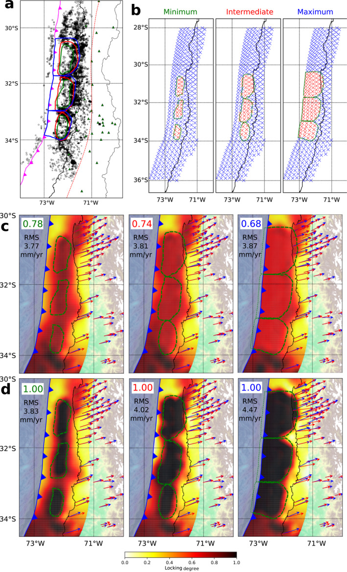
Constrained inversions of GPS data for interplate locking. (a) Definition of three sets of asperities based on the seismicity distribution. (b) These asperities are mapped onto the inversion grid for the locking inversion; the red nodes are fixed in the inversions. (c) Results of constrained inversion with optimal (i.e., lowest Bayesian Information Criterion [BIC]; see Figure 9) choice of locking for the fixed nodes of each asperity size. Green dashed lines mark the region of fixed nodes, the locking value those were fixed to is indicated in the upper left of each panel. Blue and red arrows show displacement data and model predictions, respectively. (d) Models where locking was fixed to 1 inside the asperity outlines.

In a first run, we fixed the nodes from the different asperity estimates to full coupling. Fixing them excludes these nodes from the optimization process. All other inversion parameters, such as the utilized data or Green's Functions, were the same as for the unconstrained inversion, but since the number of free parameters differed, we determined new optimal smoothing parameters (β). In order to compare the results of these inversions to the unconstrained inversion, we assessed their statistical significance using the Bayesian Information Criterion (BIC; Schwarz, 1978). The BIC allows a comparison between models with different numbers of parameters; the model with a lower BIC should be preferred. Assuming Gaussian data errors and omitting a constant term, the BIC can be expressed as

$$\text{BIC}={\chi }^2+M\ln (N),$$ (1)

where N is the number of data points, M the number of parameters and

$${\chi }^2={(\mathbf{d}-\mathbf{G}\widehat{\mathbf{m}})}^T{\mathbf{C}}_d^{-1}(\mathbf{d}-\mathbf{G}\widehat{\mathbf{m}})$$ (2)

is the chi‐square misfit. Here, d and $\widehat{\mathbf{m}}$ are the data and optimal parameter vectors, respectively; and G is the GFs matrix. It is clear from Equation 1 that the BIC will trade‐off model complexity (quantified by M) with misfit (quantified by χ ²). We assumed a diagonal data covariance matrix C _d , that is, no correlations are prescribed between data errors. The elements of C _d are ${\sigma }_i^2$, where σ _i is the error for the ith datum. We assume that data errors are dominant and assign σ _i to the GPS measurement errors.

When assuming full locking, the largest asperity size that extends all the way to the trench receives a BIC similar to (very slightly lower than) the unconstrained inversion, whereas both other geometries are clearly preferred (i.e., have a lower BIC) compared to the unconstrained inversion (see Figures 8 and 9). We also varied the prescribed locking degree for the three asperity parameterizations. For each series of inversions with the same asperity size, the number of parameters is constant, so that variations of the BIC are purely due to differences in the χ ² misfit. For all three asperity realizations, a clear preference of higher locking degrees is visible from the BIC plot. When the same number of nodes is fixed elsewhere along‐strike, the BIC minimum is situated at a significantly lower locking percentage (Figure S5 in Supporting Information S1) and is less pronounced than the overall minimum obtained with the original asperity configuration. Moreover, assuming high locking ($>$0.8) leads to a BIC larger than for the unconstrained inversion in this setup. This indicates that the data are sensitive to the along‐strike location of highly locked regions, with the location derived from microseismicity being preferred.

Figure 9.

(a) Comparison between the best‐fit constrained model with intermediate‐sized asperities (right) and the unconstrained inversion (left). Blue arrows now mark residual GPS vectors (differences between data and model). Black and white contour lines mark locking degrees of 0.7 and 0.9, respectively. Green dashed lines outline the extent of fixed nodes in the constrained inversion. (b) Histograms of station residuals in N‐S (red) and E‐W (blue) direction. (c) Bayesian Information Criterion (BIC) values for different constrained inversions for different values of fixed locking inside the three different asperity sizes. The horizontal black dashed line represents the BIC for the unconstrained inversion. The six values marked by squares are for the models shown in Figure 8.

The minima for the three asperity sizes are situated at locking values of 0.68 (maximum asperities), 0.74 (intermediate asperities), and 0.78 (minimum asperities). The global minimum BIC is reached by the largest asperity realization (i.e., with the largest number of fixed parameters), which likely implies that the inversion is underdetermined and a reduction of free parameters is preferred. Comparing data misfits and BIC values, it appears that a number of scenarios including highly coupled asperities inside the half‐ellipses outlined by the earthquakes can be fit well by the GPS data. Note that RMS data misfits of the optimum constrained models (Figure 8c) are nearly identical to the unconstrained inversion (3.73 mm/yr). While the unconstrained model shows a locking distribution with regions of higher locking that coincides with the region of elevated background microseismicity at depths of 30–45 km (especially around 32°S), the data can be fit equally well by models that concentrate coupling further updip, inside the asperity shapes we introduced. Note that some features of the unconstrained inversion in Figure 9 also show up in the constrained inversion, for instance the highly locked patch on the deeper part of the plate interface north of ∼30.5°S. This likely indicates that such a feature is required by the GPS data.

6. Discussion

Our unconstrained GPS inversion for interplate locking has demonstrated that the GPS data do not require highly coupled regions coincident with the seismicity half‐ellipses (Section 4). However, the prescription of such features yields data fits comparable to the unconstrained inversion, and our calculated BICs indicate that models with prescribed elevated locking inside the seismicity half‐ellipses are preferred. This means that the GPS data clearly do not provide evidence against the existence of such highly locked patches coincident with the aseismic zones within the half‐ellipses. Taken together with recently presented evidence from Northern Chile, where a similar microseismicity pattern preceded the 2014 M _w 8.1 Iquique earthquake (Schurr et al., 2020), we think our observations hint at a set of three adjacent highly coupled “asperities” that are present along the Central Chilean margin.

Since our conceptual model hinges on the assertion that the vast majority of the seismicity depicted in Figure 3b occurred on the plate interface, we first discuss the inherent uncertainties and the robustness of our seismicity observations (Section 6.1). After this, we present a conceptual interpretation of possibly ongoing processes on the Central Chile megathrust (Section 6.2) and discuss the temporal evolution of their seismicity signatures (Section 6.3).

6.1. Catalog Uncertainties and Robustness of Seismicity Observations

We processed raw seismic data from Central Chile and extracted 8,750 events at depths shallower than 60 km inside the time interval April 2014 to December 2018. Epicenters of these earthquakes form a pattern of three half‐ellipse shapes, open toward the trench and oriented with their long axes in trench‐parallel direction (Figure 3d and Figures S3 and S4 in Supporting Information S1). Although catalog completeness can be expected to decay offshore, analysis of retrieved magnitudes (Figure S3 in Supporting Information S1), especially of events within the “separators” and the outer rise seismicity west of the trench, shows that we should have retrieved any events with M $>3$ inside the aseismic interiors of the half‐ellipses.

The vast majority of event hypocenters are located within 10 km vertical distance from the plate interface according to slab2 (Hayes et al., 2018, see Figure 2), with the largest event numbers situated 3–5 km below the plate interface (Figure 5). Focal mechanisms uniformly show low‐angle thrusting compatible with displacement along the ∼20°–25° dipping plate interface. Moreover, most of the seismicity during the Illapel and Valparaíso earthquake sequences, which were previously interpreted to have largely occurred on the plate interface (e.g., Lange et al., 2016; Ruiz et al., 2017), also locates a similar distance below the slab2 plate interface. This may either indicate that slab2 has an offset of ∼3–5 km in this region, or that the utilized velocity model yields locations that are systematically 3–5 km too deep. Also, note that estimated relative location uncertainty in the vertical direction, a measure that does not include possible bias due to velocity model misfit, is on the order of 4 km (Figure S1 in Supporting Information S1).

Based on these considerations, we believe that a vast majority of the events that form the half‐ellipses occurred on the plate interface, and that the seismicity presented in Figure 3 largely occurs in response to active processes there. Unlike the study of Schurr et al. (2020) for the Iquique earthquake, we cannot clearly show such an ellipse pattern forming directly before a major earthquake. Due to sparse station coverage in the years 2014/2015, our catalog does not show much seismicity before the Illapel earthquake and is instead dominated by seismicity in the years 2016–2018 (Figure 4). Thus, the half‐ellipse surrounding the slip distribution of the Illapel earthquake in Figure 3 features nearly exclusively aftershock seismicity. However, analysis of seismicity from the CSN catalog (Barrientos, 2018) in the years before the Illapel earthquake (Figure 10) shows that the along‐strike seismicity “separators” that frame the Illapel earthquake to the north and south in our Figure 3 were likely already active before 2015 (the southern one is clearly present, the northern one less clear). This could imply that a late interseismic seismicity pattern akin to the one shown by Schurr et al. (2020) also preceded the Illapel earthquake. While the pre‐event seismicity signature of the Iquique and Illapel earthquakes may thus have been similar throughout most of the late interseismic stage, they clearly differ for the last weeks before the events. In the case of the 2014 Iquique earthquake, a two‐week foreshock sequence outlined the updip end of the later main shock rupture, effectively closing the seismicity ellipse (Schurr et al., 2020). Additionally, precursory aseismic slip was reported in the months leading up to the Iquique earthquake (Kato et al., 2016; Ruiz et al., 2014; Socquet et al., 2017). No such foreshock sequence or precursory activity was observed for the Illapel earthquake. The reason for this discrepancy may lie in the different updip extents of the main shock ruptures. While the Iquique earthquake reached its updip termination at ∼20 km depth (Duputel et al., 2015), there is evidence that the Illapel earthquake rupture went significantly further updip and may have extended all the way to the trench (Melgar et al., 2016; Tilmann et al., 2016).

Figure 10.

Comparison of map view seismicity distributions of events shallower than 60 km between the CSN catalog (left) and the present study (right). Since our catalog is dominated by post‐Illapel seismicity, we chose a time period before the Illapel earthquake (01/2011–06/2015) for the CSN catalog here. Note that the seismicity “separators” north and south of the Illapel rupture (i.e., at about 30.7° and 31.8°S) as well as the aseismic region roughly corresponding to the main shock rupture (Figure 3) that we found in the postseismic catalog (right) can already be recognized before the occurrence of the Illapel mainshock (left). The southernmost such feature offshore Valparaíso is largely absent in the earlier time period.

6.2. Processes on the Central Chilean Plate Interface Outlined by Seismicity

We have retrieved half‐ellipse seismicity patterns on the Central Chile megathrust that may outline regions of elevated interplate coupling (“asperities”). Similar predictions and observations of a half‐ellipse shape of microseismicity around a highly coupled region during the interseismic stage of the seismic cycle have been shown and discussed in Dmowska and Li (1982) and Schurr et al. (2020) for the case of a single asperity. Our present results may be an extension of this case to a setup of three along‐strike adjacent asperities. In the interseismic period, microseismicity on the plate interface is mostly driven by creep processes, and hence confined to regions that are not perfectly coupled (i.e., partially creeping). Multiscale heterogeneity on the fault surface means that small patches of stick‐slip motion will always be present in predominantly creeping regions, leading to creep‐driven microseismicity. Highly coupled regions on the megathrust, in contrast, are largely aseismic in the interseismic period, but produce stress concentrations along their downdip edges (Moreno et al., 2018; Schurr et al., 2020). At some point in the interseismic stage of the seismic cycle, stress along the asperity's downdip edge reaches a critical threshold, whereupon creep processes that cause microseismicity likely set in (see schematic model in Figure S6 in Supporting Information S1).

While the buildup of shear traction at the downdip end of highly coupled areas on the megathrust provides an explanation for the observed band of microseismicity at depths of 30–45 km, the seismicity “separators” between aseismic regions on the shallow megathrust (Figure 3b) require a different explanation. Understanding why and where these separators occur is crucial, since they appear to prescribe, or at least image, along‐strike segmentation of the Central Chilean plate interface. Along‐strike changes in plate interface behavior are thought to be primarily controlled by plate interface roughness, which is often a consequence of the subduction of seafloor relief (Bassett & Watts, 2015; van Rijsingen et al., 2019). Features like ridges or fracture zones on the downgoing plate may also be more hydrated than ordinary oceanic crust, which can cause elevated pore fluid pressure leading to reduced interplate coupling on the megathrust (Moreno et al., 2014). Clearly identifiable seafloor features, the CFZ and JFR (Figures 1 and 3), likely acted as delimiters of the 2015 Illapel earthquake (Figure 3b, Lange et al., 2016; Poli et al., 2017; Tilmann et al., 2016). The microseismicity extending to shallow depths we observe both north and south of the Illapel rupture (Figures 3b and 3c) could thus be linked to the ongoing subduction of these features. The southernmost separator, located at ∼33°S, is observed where the San Antonio seamount is currently being subducted (Ruiz et al., 2018). We note that while the separator just north of 32°S appears to roughly coincide with the northern edge of the JFR's projection, the entire JFR is much wider and extends across most of the central seismicity half‐ellipse we observe, a region we associate with high coupling. Since we do not know the properties of the already subducted continuation of the JFR, which is a heterogeneous feature offshore (Figure 1), it is possible that the separator near 32°S represents a specific feature (e.g., one or several seamounts) on the already subducted JFR, or that the edge of the ridge is more efficient at lowering interplate coupling than its center.

Increased lower plate roughness and/or higher pore fluid pressure on the plate interface usually leads to reduced interplate coupling and thus to a larger proportion of aseismic creep (Wang & Bilek, 2014). This fits our observation of more repeating earthquakes in the separators compared to other regions (Figures 3b and 3c; also see Poli et al., 2017; Ruiz et al., 2017). Events with highly similar waveforms are a consequence of ongoing aseismic creep processes that drive seismic slip on small coupled patches along the heterogeneous plate interface (Nadeau & McEvilly, 1999; Uchida & Bürgmann, 2019). While available maps of interplate coupling (Figure 6, Métois et al., 2012) have insufficient resolution to show reduced coupling along such narrow segments in our study area (Figure 7), the region north of the 2015 Illapel earthquake showcases larger‐scale decreased interplate locking accompanied by widespread seismicity (including repeaters) along most of the plate interface (Figures 3b and 3c). Seismicity along the separators is episodic (Figure 3c) and mostly part of major earthquake sequences (Illapel, Valparaíso). However, there is evidence for swarm‐like earthquake sequences north and south of the later Illapel rupture in the decades before its rupture (Poli et al., 2017) as well as at ∼33°S in the years before the Maule earthquake (Holtkamp & Brudzinski, 2014). Both separators can be recognized in seismicity plots of the CSN earthquake catalog before 2014 (Figure 10). Moreover, some repeating earthquakes are observed from 04/2014 (i.e., before Illapel) in both separators (Figure 3c), and the area of the 2017 Valparaíso earthquake was activated during the Illapel sequence in 2015. The 2017 Valparaíso sequence itself was preceded by transient deformation recognized in GPS data as well as a foreshock sequence (Ruiz et al., 2017). North of our study region, the 2020 Atacama seismic sequence, located in a narrow region of low interplate coupling at the southern edge of where the Copiapo Ridge enters the subduction (Klein et al., 2021), may present another more recent example of episodic seismic activity along a possible separator.

We thus think that the seismicity separators we observe represent areas of locally decreased interplate coupling and thus increased aseismic creep along the plate interface, often prescribed by features on the incoming oceanic plate. They are intermittently active during the interseismic stage and more strongly active in the postseismic stage of one of the adjacent asperities, when their activity is driven by postseismic slip and possibly stress concentrations at the along‐strike terminations of the main shock rupture. Given a long enough observation timespan in the interseismic period, the overall seismicity distribution should resemble the postseismic one (compare the half‐ellipse outlined by Illapel aftershocks to the one south of it; Figure S4 in Supporting Information S1), which would imply that the localized lows in interseismic coupling that define these separators are stable throughout the seismic cycle and mainly due to structure on the downgoing plate (as also argued in Agurto‐Detzel et al., 2019). It is important to better characterize such regions, for instance through the deployment of dense GPS networks (ideally on‐ and offshore), since their widths relative to the adjacent highly coupled areas and their coupling properties determine their efficiency as barriers to large earthquakes (e.g., Corbi et al., 2017).

6.3. Mogi Doughnuts and the Temporal Evolution of Seismicity Patterns

Pre‐seismic quiescence in an earthquake's rupture area, accompanied by increased seismicity levels in a ring or half‐ring shape around it, has been first observed more than five decades ago (Kanamori, 1981; Mogi, 1969, 1979). Although such “Mogi doughnuts” have later also been predicted with mechanical models (Dmowska & Li, 1982) and observed in rock mechanics experiments (Goebel et al., 2012), only very few clear observations of Mogi doughnuts have been made to date (e.g., Schurr et al., 2020). In contrast, observations of aftershock seismicity surrounding the main shock slip areas are well established (Das & Henry, 2003) and often ascribed to stress concentrations at the rupture limits.

We think that one reason for the scarce observations of Mogi Doughnuts may lie in the temporal evolution of seismicity, which appears to be markedly different between the downdip edges of highly coupled regions and the along‐strike separators. Interseismic loading of asperities naturally results in concentrations of shear traction at their downdip edges (e.g., Moreno et al., 2018). Microseismicity at these stress concentrations likely only commences once a stress threshold level has been reached. From that time onwards, seismicity in these regions will appear to be continuous (Figure 3c). Observations of such bands of seismicity located around the downdip termination of interseismic locking are not uncommon (e.g., Ader et al., 2012; Feng et al., 2012; Yarce et al., 2019). The along‐strike separators that subdivide the shallower megathrust into single asperities, in contrast, are only active in episodically occurring bursts (Figure 3c), most prominently when activated by nearby events (similar to observations of Schurr et al., 2020). This means that for relatively short‐term seismicity studies like ours, such separators can easily be missed. Unlike the band of deeper interface seismicity, they feature large amounts of repeating earthquakes that are proxies for ongoing aseismic creep. Long‐term studies of repeating earthquakes have shown clusters of such events downdip and at the along‐strike terminations of later megathrust earthquakes (e.g., Uchida & Matsuzawa, 2013). These observations may be due to the erosion of coupled asperities by creep processes that have been shown in rate‐and‐state simulations (Jiang & Lapusta, 2017; Mavrommatis et al., 2017).

Immediately after a main shock rupture on an adjacent segment occurs, its along‐strike separators will show high rates of seismicity (see Figure 3c) due to induced stress concentrations at the rupture edges as well as high‐rate aseismic processes in the postseismic stage (Perfettini et al., 2010). Thus, a clearer and easier identification of such separators during aftershock series is possible due to higher seismicity rates. We think that the general pattern of microseismicity is, however, similar for the postseismic and the interseismic stage of the seismic cycle, because the features that prescribe the interseismic seismicity pattern (regions of only partial coupling acting as along‐strike separators and the downdip edges of asperities that concentrate stresses) also prescribe the edges of the main shock rupture. As both aftershock series and postseismic afterslip to first order occur in the region surrounding main shock slip (e.g., Das & Henry, 2003; Perfettini et al., 2010), both creep‐driven or stress‐driven aftershock seismicity should outline patterns that are to first order similar to what emerges when a sufficiently large proportion of the interseismic stage is observed. A recent example for the postseismic activation of along‐strike separators is the 2016 M _w 7.8 Pedernales earthquake in Ecuador, where the main shock was located on the deeper part of the megathrust, but activated three narrow seismicity separators outlining largely aseismic regions on the presumably unruptured shallow part of the megathrust (Agurto‐Detzel et al., 2019; Soto‐Cordero et al., 2020). As in Central Chile, these features can be correlated with incoming seafloor relief.

For Central Chile, our results imply that two adjacent asperities are possibly present between the rupture areas of the 2015 Illapel and the 2010 Maule earthquake (see Figure 3b), and may have accumulated stress for nearly 300 years. Given that the 2014 Iquique earthquake was preceded by a similar pattern (Schurr et al., 2020), we believe that our observations could help to constrain the seismic potential of the region. The imaged barrier between the two potential asperities, highlighted by the 2017 Valparaíso earthquake sequence (Figures 3b and 3c), likely mechanically controls whether they will rupture jointly or individually.

7. Conclusions

We observe three trenchward open seismicity half‐ellipses on the Central Chile megathrust when analyzing the time period 2014–2018. They consist of a trench‐parallel, along‐strike continuous band of plate interface microseismicity at depths of 30–45 km, as well as two along‐strike separators where seismicity extends significantly further toward the trench. The resolution of available GPS data does not allow us to independently verify whether these half‐ellipses correspond to strongly coupled patches on the megathrust. However, by prescribing such highly locked “asperities” in constrained inversions of GPS data, we show that their existence is one possible way to explain the observed upper plate deformation in Central Chile.

According to our interpretation, continued interseismic loading of strongly coupled asperities leads to gradual buildup of stress concentrations along their downdip edges. These stress concentrations eventually cause aseismic creep driving continuous microseismicity from some time in the interseismic stage onwards. The narrow along‐strike separators between asperities appear to correspond to regions of increased roughness and/or hydration on the incoming Nazca Plate, likely effecting elevated creep that occurs in transient bursts and drives swarm‐like earthquake sequences. This implies that valuable information about the segmentation of megathrust faults can be obtained from the analysis of seismicity distributions, provided that the analyzed region has already overcome the stress threshold after which the microseismicity in the downdip band develops, and that the observational timespan is long enough to capture the episodic activity of along‐strike separators. We further speculate that incorporating seismicity information into future locking inversion approaches may be a way to improve spatial resolution of GPS‐based locking maps, especially in the badly resolved offshore regions.

Supporting information

Supporting Information S1

Sippl, C. , Moreno, M. , & Benavente, R. (2021). Microseismicity appears to outline highly coupled regions on the Central Chile megathrust. Journal of Geophysical Research: Solid Earth, 126, e2021JB022252. 10.1029/2021JB022252

Data Availability Statement

The seismic waveform data that was used to compile the earthquake catalog was retrieved from the IRIS webpage (http://www.ds.iris.edu/ds/nodes/dmc/), and came from the networks C1 (Universidad de Chile, 2013), C (no DOI available), II (Scripps Institution of Oceanography, 1986), G (Institut de Physique du Globe de Paris & Ecole et Observatoire des Sciences de la Terre de Strasbourg (EOST), 1982) and WA (Universidad Nacional de San Juan Argentina, 1958). Moment tensors shown in Figure 3 were retrieved from the globalCMT (https://www.globalcmt.org/) and GEOFON (https://geofon.gfz-potsdam.de/eqinfo/) databases. Seismic data processing was done with ObsPy (Beyreuther et al., 2010), figures were plotted with the Matplotlib (Hunter, 2007) and Basemap (https://matplotlib.org/basemap/) libraries. The seismicity catalog presented in this article is available on Zenodo.org (https://dx.doi.org/10.5281/zenodo.5569275).

References

- Aagaard, B. T. , Knepley, M. G. , & Williams, C. A. (2013). A domain decomposition approach to implementing fault slip in finite‐element models of quasi‐static and dynamic crustal deformation. Journal of Geophysical Research, 118(6), 3059–3079. 10.1002/jgrb.50217 [DOI] [Google Scholar]
- Ader, T. , Avouac, J.‐P. , Liu‐Zeng, J. , Lyon‐Caen, H. , Bollinger, L. , Galetzka, J. , et al. (2012). Convergence rate across the Nepal Himalaya and interseismic coupling on the Main Himalayan Thrust: Implications for seismic hazard. Journal of Geophysical Research, 117(4), 1–16. 10.1029/2011JB009071 [DOI] [Google Scholar]
- Agurto‐Detzel, H. , Font, Y. , Charvis, P. , Régnier, M. , Rietbrock, A. , Ambrois, D. , et al. (2019). Ridge subduction and afterslip control aftershock distribution of the 2016 Mw 7.8 Ecuador earthquake. Earth and Planetary Science Letters, 520, 63–76. 10.1016/j.epsl.2019.05.029 [DOI] [Google Scholar]
- Anderson, M. , Alvarado, P. , Zandt, G. , & Beck, S. L. (2007). Geometry and brittle deformation of the subducting Nazca Plate, Central Chile and Argentina. Geophysical Journal International, 171(1), 419–434. 10.1111/j.1365-246X.2007.03483.x [DOI] [Google Scholar]
- Angermann, D. , Klotz, J. , & Reigber, C. (1999). Space‐geodetic estimation of the Nazca‐South America Euler vector. Earth and Planetary Science Letters, 171(3), 329–334. 10.1016/S0012-821X(99)00173-9 [DOI] [Google Scholar]
- Barrientos, S. (2018). The seismic network of Chile. Seismological Research Letters, 89(2A), 467–474. 10.1785/0220160195.1785/0220160195 [DOI] [Google Scholar]
- Barrientos, S. , Vera, E. , Alvarado, P. , & Monfret, T. (2004). Crustal seismicity in central Chile. Journal of South American Earth Sciences, 16(8), 759–768. 10.1016/j.jsames.2003.12.001 [DOI] [Google Scholar]
- Bassett, D. , & Watts, A. B. (2015). Gravity anomalies, crustal structure, and seismicity at subduction zones: 1. Seafloor roughness and subducting relief. Geochemistry, Geophysics, Geosystems, 16, 1508–1540. 10.1002/2014gc005684 [DOI] [Google Scholar]
- Béjar‐Pizarro, M. , Socquet, A. , Armijo, R. , Carrizo, D. , Genrich, J. , & Simons, M. (2013). Andean structural control on interseismic coupling in the North Chile subduction zone. Nature Geoscience, 6(6), 462–467. 10.1038/ngeo1802 [DOI] [Google Scholar]
- Benavente, R. , Cummins, P. R. , & Dettmer, J. (2016). Rapid automated W‐phase slip inversion for the Illapel great earthquake (2015, Mw = 8.3). Geophysical Research Letters, 43(5), 1910–1917. 10.1002/2015GL067418 [DOI] [Google Scholar]
- Beyreuther, M. , Barsch, R. , Krischer, L. , Megies, T. , Behr, Y. , & Wassermann, J. (2010). ObsPy: A Python toolbox for seismology. Seismological Research Letters, 81(3), 530–533. 10.1785/gssrl.81.3.530 [DOI] [Google Scholar]
- Bletery, Q. , Thomas, A. M. , Rempel, A. W. , Karlstrom, L. , Sladen, A. , & De Barros, L. (2016). Mega‐earthquakes rupture flat megathrusts. Science, 354(6315), 1027–1031. 10.1785/gssrl.81.3.530 [DOI] [PubMed] [Google Scholar]
- Bravo, F. , Koch, P. , Riquelme, S. , Fuentes Serrano, M. , & Campos, J. (2019). Slip distribution of the 1985 Valparaíso earthquake constrained with seismic and deformation data. Seismological Research Letters, 9, 1–9. 10.1785/0220180396 [DOI] [Google Scholar]
- Brooks, B. , Bevis, M. , Smalley, R. , Kendrick, E. , Manceda, R. , Lauría, E. , & Araujo, M. (2003). Crustal motion in the Southern Andes (26‐36S): Do the Andes behave like a microplate? Geochemistry, Geophysics, Geosystems, 4(10), 1–14. 10.1029/2003GC000505 [DOI] [Google Scholar]
- Bürgmann, R. , Kogan, M. G. , Steblov, G. M. , Hilley, G. , Levin, V. , & Apel, E. (2005). Interseismic coupling and asperity distribution along the Kamchatka subduction zone. Journal of Geophysical Research, 110(7), B07405. 10.1029/2005JB003648 [DOI] [Google Scholar]
- Carvajal, M. , Cisternas, M. , & Catalán, P. A. (2017). Source of the 1730 Chilean earthquake from historical records: Implications for the future tsunami hazard on the coast of Metropolitan Chile. Journal of Geophysical Research, 122(5), 3648–3660. 10.1002/2017JB014063 [DOI] [Google Scholar]
- Chlieh, M. , Avouac, J.‐P. , Sieh, K. , Natawidjaja, D. H. , & Galetzka, J. (2008). Heterogeneous coupling of the Sumatran megathrust constrained by geodetic and paleogeodetic measurements. Journal of Geophysical Research, 113(5), B05305. 10.1029/2007JB004981 [DOI] [Google Scholar]
- Chlieh, M. , De Chabalier, J. B. , Ruegg, J. C. , Armijo, R. , Dmowska, R. , Campos, J. , & Feigl, K. L. (2004). Crustal deformation and fault slip during the seismic cycle in the North Chile subduction zone, from GPS and InSAR observations. Geophysical Journal International, 158(2), 695–711. 10.1111/j.1365-246X.2004.02326.x [DOI] [Google Scholar]
- Chlieh, M. , Perfettini, H. , Tavera, H. , Avouac, J.‐P. , Remy, D. , Nocquet, J. M. , & Bonvalot, S. (2011). Interseismic coupling and seismic potential along the Central Andes subduction zone. Journal of Geophysical Research, 116(12), B12405. 10.1029/2010JB008166 [DOI] [Google Scholar]
- Cloos, M. (1992). Thrust‐type subduction‐zone earthquakes and seamount asperities: A physical model for seismic rupture. Geology, 20, 601–604. [Google Scholar]
- Comte, D. , & Pardo, M. (1991). Reappraisal of great historical earthquakes in the northern Chile and southern Peru seismic gaps. Natural Hazards, 4(1), 23–44. [DOI] [Google Scholar]
- Contreras‐Reyes, E. , & Carrizo, D. (2011). Control of high oceanic features and subduction channel on earthquake ruptures along the Chile‐Peru subduction zone. Physics of the Earth and Planetary Interiors, 186(1–2), 49–58. 10.1016/j.pepi.2011.03.002 [DOI] [Google Scholar]
- Corbi, F. , Funiciello, F. , Brizzi, S. , Lallemand, S. , & Rosenau, M. (2017). Control of asperities size and spacing on seismic behavior of subduction megathrusts. Geophysical Research Letters, 44(16), 8227–8235. 10.1002/2017GL074182 [DOI] [Google Scholar]
- Das, S. , & Henry, C. (2003). Spatial relation between main earthquake slip and its aftershock distribution. Reviews of Geophysics, 41(3), 1013. 10.1029/2002RG000119 [DOI] [Google Scholar]
- Di Stefano, R. , Aldersons, F. , Kissling, E. , Baccheschi, P. , Chiarabba, C. , & Giardini, D. (2006). Automatic seismic phase picking and consistent observation error assessment: Application to the Italian seismicity. Geophysical Journal International, 165(1), 121–134. 10.1111/j.1365-246X.2005.02799.x [DOI] [Google Scholar]
- Diehl, T. , Deichmann, N. , Kissling, E. , & Husen, S. (2009). Automatic S‐wave picker for local earthquake tomography. Bulletin of the Seismological Society of America, 99(3), 1906–1920. 10.1785/0120080019 [DOI] [Google Scholar]
- Dmowska, R. , & Li, V. C. (1982). A mechanical model of precursory source processes for some large earthquakes. Geophysical Research Letters, 9(4), 393–396. 10.1029/GL009i004p00393 [DOI] [Google Scholar]
- Duputel, Z. , Jiang, J. , Jolivet, R. , Simons, M. , Rivera, L. , Ampuero, J. P. , & Minson, S. E. (2015). The Iquique earthquake sequence of April 2014: Bayesian modeling accounting for prediction uncertainty. Geophysical Research Letters, 42(19), 7949–7957. 10.1002/2015GL065402 [DOI] [Google Scholar]
- Feng, L. , Newman, A. V. , Protti, M. , Gonzalez, V. , Jiang, Y. , & Dixon, T. (2012). Active deformation near the Nicoya Peninsula, northwestern Costa Rica, between 1996 and 2010: Interseismic megathrust coupling. Journal of Geophysical Research, 117(6), 1–23. 10.1029/2012JB009230 [DOI] [Google Scholar]
- Fujiwara, T. , Kodaira, S. , No, T. , Kaiho, Y. , Takahashi, N. , & Kaneda, Y. (2011). The 2011 Tohoku‐oki Earthquake: Displacement reaching the trench axis. Science, 334, 1240. [DOI] [PubMed] [Google Scholar]
- GEBCO Compilation Group . (2020). GEBCO 2020 grid. 10.5285/a29c5465-b138-234d-e053-6c86abc040b9 [DOI]
- Goebel, T. H. , Becker, T. W. , Schorlemmer, D. , Stanchits, S. , Sammis, C. G. , Rybacki, E. , & Dresen, G. (2012). Identifying fault heterogeneity through mapping spatial anomalies in acoustic emission statistics. Journal of Geophysical Research, 117(3), 1–18. 10.1029/2011JB008763 [DOI] [Google Scholar]
- Hayes, G. P. , Moore, G. , Portner, D. E. , Hearne, M. , Flamme, H. , Furtney, M. , & Smoczyk, G. M. (2018). Slab2, a comprehensive subduction zone geometry model. Science, 362(6410), 58–61. 10.1126/science.aat4723 [DOI] [PubMed] [Google Scholar]
- Hayes, G. P. , Wald, D. J. , & Johnson, R. L. (2012). Slab1.0: A three‐dimensional model of global subduction zone geometries. Journal of Geophysical Research, 117(1), 1–15. 10.1029/2011JB008524 [DOI] [Google Scholar]
- Holtkamp, S. , & Brudzinski, M. R. (2014). Megathrust earthquake swarms indicate frictional changes which delimit large earthquake ruptures. Earth and Planetary Science Letters, 390, 234–243. 10.1016/j.epsl.2013.10.033 [DOI] [Google Scholar]
- Hunter, J. D. (2007). Matplotlib: A 2D graphics environment. Computing in Science & Engineering, 9(3), 90–95. 10.1109/MCSE.2007.55 [DOI] [Google Scholar]
- Ide, S. , Baltay, A. , & Beroza, G. C. (2011). Shallow dynamic overshoot and energetic deep rupture in the 2011 Mw 9.0 Tohoku‐Oki earthquake. Science, 332(6036), 1426–1429. 10.1126/science.1207020 [DOI] [PubMed] [Google Scholar]
- Institut de Physique du Globe de Paris & Ecole et Observatoire des Sciences de la Terre de Strasbourg (EOST) . (1982). GEOSCOPE ‐ French Global Network of broadband seismic stations. 10.18715/GEOSCOPE [DOI]
- Jiang, J. , & Lapusta, N. (2017). Connecting depth limits of interseismic locking, microseismicity, and large earthquakes in models of long‐term fault slip. Journal of Geophysical Research: Solid Earth, 122(8), 6491–6523. 10.1002/2017JB014030 [DOI] [Google Scholar]
- Kanamori, H. (1981). The nature of seismicity patterns before large earthquakes. In Earthquake prediction (pp. 1–19). 10.1029/me004p0001 [DOI] [Google Scholar]
- Kato, A. , Fukuda, J. , Kumazawa, T. , & Nakagawa, S. (2016). Accelerated nucleation of the 2014 Iquique, Chile Mw 8.2 earthquake. Scientific Reports, 6, 1–9. 10.1038/srep24792 [DOI] [PMC free article] [PubMed] [Google Scholar]
- Kendrick, E. , Bevis, M. , Smalley, R. , Brooks, B. , Vargas, R. B. , Lauría, E. , & Fortes, L. P. S. (2003). The Nazca‐South America Euler vector and its rate of change. Journal of South American Earth Sciences, 16(2), 125–131. 10.1016/S0895-9811(03)00028-2 [DOI] [Google Scholar]
- Kissling, E. , Ellsworth, W. L. , Eberhart‐Phillips, D. , & Kradolfer, U. (1994). Initial reference models in local earthquake tomography. Journal of Geophysical Research, 99, 19646. [Google Scholar]
- Klein, E. , Potin, B. , Pasten‐Araya, F. , Tissandier, R. , Azua, K. , Duputel, Z. , & Vigny, C. (2021). Interplay of seismic and a‐seismic deformation during the 2020 sequence of Atacama , Chile. Earth and Planetary Science Letters, 570, 117081. 10.1029/93jb03138 [DOI] [Google Scholar]
- Klotz, J. , Khazaradze, G. , Angermann, D. , Reigber, C. , Perdomo, R. , & Cifuentes, O. (2001). Earthquake cycle dominates contemporary crustal deformation in Central and Southern Andes. Earth and Planetary Science Letters, 193(3–4), 437–446. 10.1016/S0012-821X(01)00532-5 [DOI] [Google Scholar]
- Lange, D. , Geersen, J. , Barrientos, S. , Moreno, M. , Grevemeyer, I. , Contreras‐Reyes, E. , & Kopp, H. (2016). Aftershock seismicity and tectonic setting of the 2015 September 16 Mw 8.3 Illapel earthquake, Central Chile. Geophysical Journal International, 206(2), 1424–1430. 10.1093/gji/ggw218 [DOI] [Google Scholar]
- Lange, D. , Tilmann, F. , Barrientos, S. , Contreras‐Reyes, E. , Methe, P. , Moreno, M. , & Beck, S. L. (2012). Aftershock seismicity of the 27 February 2010 Mw 8.8 Maule earthquake rupture zone. Earth and Planetary Science Letters, 317–318, 413–425. 10.1016/j.epsl.2011.11.034 [DOI] [Google Scholar]
- Lay, T. , & Kanamori, H. (1981). An asperity model for large earthquake sequences. Earthquake prediction (pp. 579–592). American Geophysical Union. [Google Scholar]
- Lay, T. , Kanamori, H. , Ammon, C. J. , Koper, K. D. , Hutko, A. R. , Ye, L. , et al. (2012). Depth‐varying rupture properties of subduction zone megathrust faults. Journal of Geophysical Research, 117(4), B04311. 10.1029/2011JB009133 [DOI] [Google Scholar]
- Li, S. , Moreno, M. , Bedford, J. , Rosenau, M. , & Oncken, O. (2015). Revisiting viscoelastic effects on interseismic deformation and locking degree: A case study of the Peru‐North Chile subduction zone. Journal of Geophysical Research, 120(6), 4522–4538. 10.1002/2015JB011903 [DOI] [Google Scholar]
- Lomnitz, C. (2004). Major Earthquakes of Chile: A Historical Survey, 1535‐1960. Seismological Research Letters, 75(3), 368–378. 10.1785/gssrl.75.3.368 [DOI] [Google Scholar]
- Loveless, J. P. , & Meade, B. J. (2011). Spatial correlation of interseismic coupling and coseismic rupture extent of the 2011 MW = 9.0 Tohoku‐oki earthquake. Geophysical Research Letters, 38(17), 2–6. 10.1029/2011GL048561 [DOI] [Google Scholar]
- Loveless, J. P. , & Meade, B. J. (2016). Two decades of spatiotemporal variations in subduction zone coupling offshore Japan. Earth and Planetary Science Letters, 436, 19–30. 10.1016/j.epsl.2015.12.033 [DOI] [Google Scholar]
- Marot, M. , Monfret, T. , Pardo, M. , Ranalli, G. , & Nolet, G. (2013). A double seismic zone in the subducting Juan Fernandez Ridge of the Nazca Plate (32S), central Chile. Journal of Geophysical Research, 118(7), 3462–3475. 10.1002/jgrb.50240 [DOI] [Google Scholar]
- Mavrommatis, A. P. , Segall, P. , & Johnson, K. M. (2017). A physical model for interseismic erosion of locked fault asperities. Journal of Geophysical Research: Solid Earth, 122(10), 8326–8346. 10.1002/2017JB014533 [DOI] [Google Scholar]
- Melgar, D. , Fan, W. , Riquelme, S. , Geng, J. , Liang, C. , Fuentes Serrano, M. , & Fielding, E. J. (2016). Slip segmentation and slow rupture to the trench during the 2015, Mw8.3 Illapel, Chile earthquake. Geophysical Research Letters, 43(3), 961–966. 10.1002/2015GL067369 [DOI] [Google Scholar]
- Métois, M. , Socquet, A. , & Vigny, C. (2012). Interseismic coupling, segmentation and mechanical behavior of the central Chile subduction zone. Journal of Geophysical Research, 117(3), B03406. 10.1029/2011JB008736 [DOI] [Google Scholar]
- Métois, M. , Vigny, C. , & Socquet, A. (2016). Interseismic coupling, megathrust earthquakes and seismic swarms along the Chilean subduction zone (38–18S). Pure and Applied Geophysics, 173(5), 1431–1449. 10.1007/s00024-016-1280-5 [DOI] [Google Scholar]
- Mogi, K. (1969). Some features of recent seismic activity in and near Japan(2): Activity before and after great earthquakes (pp. 395–417). Bulletin of the Earthquake Research Institute, The University of Tokyo. [Google Scholar]
- Mogi, K. (1979). Two kinds of seismic gaps. Pure and Applied Geophysics, 117(6), 1172–1186. 10.1007/BF00876213 [DOI] [Google Scholar]
- Moreno, M. , Haberland, C. , Oncken, O. , Rietbrock, A. , Angiboust, S. , & Heidbach, O. (2014). Locking of the Chile subduction zone controlled by fluid pressure before the 2010 earthquake. Nature Geoscience, 7(4), 292–296. 10.1038/ngeo2102 [DOI] [Google Scholar]
- Moreno, M. , Li, S. , Melnick, D. , Bedford, J. , Baez, J. C. , Motagh, M. , et al. (2018). Chilean megathrust earthquake recurrence linked to frictional contrast at depth. Nature Geoscience, 11(4), 285–290. 10.1038/s41561-018-0089-5 [DOI] [Google Scholar]
- Moreno, M. , Melnick, D. , Rosenau, M. , Baez, J. C. , Klotz, J. , Oncken, O. , et al. (2012). Toward understanding tectonic control on the Mw 8.8 2010 Maule Chile earthquake. Earth and Planetary Science Letters, 321–322, 152–165. 10.1016/j.epsl.2012.01.006 [DOI] [Google Scholar]
- Moreno, M. , Melnick, D. , Rosenau, M. , Bolte, J. , Klotz, J. , Echtler, H. , et al. (2011). Heterogeneous plate locking in the South‐Central Chile subduction zone: Building up the next great earthquake. Earth and Planetary Science Letters, 305(3–4), 413–424. 10.1016/j.epsl.2011.03.025 [DOI] [Google Scholar]
- Moreno, M. , Rosenau, M. , & Oncken, O. (2010). 2010 Maule earthquake slip correlates with pre‐seismic locking of Andean subduction zone. Nature, 467(7312), 198–202. 10.1038/nature09349 [DOI] [PubMed] [Google Scholar]
- Müller, R. D. , Sdrolias, M. , Gaina, C. , & Roest, W. R. (2008). Age, spreading rates, and spreading asymmetry of the world’s ocean crust. Geochemistry, Geophysics, Geosystems, 9(4), Q04006. 10.1029/2007GC001743 [DOI] [Google Scholar]
- Nadeau, R. M. , & McEvilly, T. V. (1999). Fault slip rates at depth from recurrence intervals of repeating microearthquakes. Science, 285(5428), 718–721. 10.1126/science.285.5428.718 [DOI] [PubMed] [Google Scholar]
- Nealy, J. L. , Herman, M. W. , Moore, G. , Hayes, G. P. , Benz, H. , Bergman, E. , & Barrientos, S. (2017). Valparaíso earthquake sequence and the megathrust patchwork of central Chile. Geophysical Research Letters, 44(17), 8865–8872. 10.1002/2017GL074767 [DOI] [Google Scholar]
- Oleskevich, D. A. , Hyndman, R. D. , & Wang, K. (1999). The updip and downdip limits to great subduction earthquakes: Thermal and structural models of Cascadia, south Alaska, SW Japan, and Chile. Journal of Geophysical Research, 104(B7), 14965–14991. 10.1029/1999jb900060 [DOI] [Google Scholar]
- Pacheco, F. , Sykes, L. R. , & Scholz, C. H. (1993). Nature of seismic coupling along simple plate boundaries of the subduction type. Journal of Geophysical Research, 98, 14159. [Google Scholar]
- Perfettini, H. , Avouac, J.‐P. , Tavera, H. , Kositsky, A. , Nocquet, J. M. , Bondoux, F. , et al. (2010). Seismic and aseismic slip on the Central Peru megathrust. Nature, 465(7294), 78–81. 10.1029/93jb00349 [DOI] [PubMed] [Google Scholar]
- Poli, P. , Jeria, A. M. , & Ruiz, S. (2017). The Mw 8.3 lllapel earthquake (Chile): Preseismic and postseismic activity associated with hydrated slab structures. Geology, 45(3), 247–250. 10.1130/G38522.1 [DOI] [Google Scholar]
- Ramos, V. A. , Cristallini, E. O. , & Pérez, D. J. (2002). The Pampean flat‐slab of the Central Andes. Journal of South American Earth Sciences, 15(1), 59–78. 10.1016/S0895-9811(02)00006-8 [DOI] [Google Scholar]
- Ramos, V. A. , & Folguera, A. (2009). Andean flat‐slab subduction through time. Geological Society, London, Special Publications, 327(1), 31–54. 10.1144/sp327.3 [DOI] [Google Scholar]
- Ruiz, J. , Contreras‐Reyes, E. , Ortega Culaciati, F. , & Manríquez, P. (2018). Rupture process of the April 24, 2017, Mw 6.9 Valparaíso earthquake from the joint inversion of teleseismic body waves and near‐field data. Physics of the Earth and Planetary Interiors, 279, 1–14. 10.1016/j.pepi.2018.03.007 [DOI] [Google Scholar]
- Ruiz, S. , Aden‐Antoniow, F. , Baez, J. C. , Otarola, C. , Potin, B. , del Campo, F. , et al. (2017). Nucleation phase and dynamic inversion of the Mw 6.9 Valparaíso 2017 Earthquake in Central Chile. Geophysical Research Letters, 44, 10297. 10.1002/2017GL075675 [DOI] [Google Scholar]
- Ruiz, S. , & Madariaga, R. (2018). Historical and recent large megathrust earthquakes in Chile. Tectonophysics, 733, 37–56. 10.1016/j.tecto.2018.01.015 [DOI] [Google Scholar]
- Ruiz, S. , Metois, M. , Fuenzalida, A. , Ruiz, J. , Leyton, F. , Grandin, R. , et al. (2014). Intense foreshocks and a slow slip event preceded the 2014 Iquique Mw 8.1 earthquake. Science, 345, 1165–1170. [DOI] [PubMed] [Google Scholar]
- Savage, J. C. (1983). A dislocation model of strain accumulation and release at a subduction zone. Journal of Geophysical Research, 88(B6), 4984–4996. 10.1126/science.1256074 [DOI] [Google Scholar]
- Schurr, B. , Asch, G. , Hainzl, S. , Bedford, J. , Hoechner, A. , Palo, M. , et al. (2014). Gradual unlocking of plate boundary controlled initiation of the 2014 Iquique earthquake. Nature, 512(7514), 299–302. 10.1038/nature13681 [DOI] [PubMed] [Google Scholar]
- Schurr, B. , Moreno, M. , Tréhu, A. M. , Bedford, J. , Kummerow, J. , Li, S. , & Oncken, O. (2020). Forming a Mogi doughnut in the years prior to and immediately before the 2014 M8.1 Iquique, Northern Chile, Earthquake. Geophysical Research Letters, 47(16). 10.1029/2020GL088351 [DOI] [Google Scholar]
- Schwarz, G. (1978). Estimating the dimension of a model. Annals of Statistics, 6(2), 461–464. 10.1214/aos/1176348654 [DOI] [Google Scholar]
- Scripps Institution of Oceanography . (1986). IRIS/IDA seismic network. International Federation of Digital Seismograph Networks. 10.1214/aos/1176344136 [DOI] [Google Scholar]
- Sippl, C. , Schurr, B. , Yuan, X. , Mechie, J. , Schneider, F. M. , Gadoev, M. , et al. (2013). Geometry of the Pamir‐Hindu Kush intermediate‐depth earthquake zone from local seismic data. Journal of Geophysical Research, 118(4), 1438–1457. 10.1002/jgrb.50128 [DOI] [Google Scholar]
- Socquet, A. , Valdes, J. P. , Jara, J. , Cotton, F. , Walpersdorf, A. , Cotte, N. , et al. (2017). An 8 month slow slip event triggers progressive nucleation of the 2014 Chile megathrust. Geophysical Research Letters, 44(9), 4046–4053. 10.1002/2017GL073023 [DOI] [Google Scholar]
- Soto‐Cordero, L. , Meltzer, A. , Bergman, E. , Hoskins, M. , Stachnik, J. C. , Agurto‐Detzel, H. , et al. (2020). Structural control on megathrust rupture and slip behavior: Insights from the 2016 Mw 7.8 Pedernales Ecuador Earthquake. Journal of Geophysical Research: Solid Earth, 125. 10.1029/2019JB018001 [DOI] [Google Scholar]
- Sparkes, R. , Tilmann, F. , Hovius, N. , & Hillier, J. (2010). Subducted seafloor relief stops rupture in South American great earthquakes: Implications for rupture behaviour in the 2010 Maule, Chile earthquake. Earth and Planetary Science Letters, 298(1–2), 89–94. 10.1016/j.epsl.2010.07.029 [DOI] [Google Scholar]
- Sykes, L. R. (1971). Aftershock zones of great earthquakes, seismicity gaps, and earthquake prediction for Alaska and the Aleutians. Journal of Geophysical Research, 76(32), 8021–8041. 10.1029/jb076i032p08021 [DOI] [Google Scholar]
- Tassara, A. , & Echaurren, A. (2012). Anatomy of the Andean subduction zone: Three‐dimensional density model upgraded and compared against global‐scale models. Geophysical Journal International, 189(1), 161–168. 10.1111/j.1365-246X.2012.05397.x [DOI] [Google Scholar]
- Thurber, C. H. , & Eberhart‐Phillips, D. (1999). Local earthquake tomography with flexible gridding. Computers & Geosciences, 25(7), 809–818. 10.1016/S0098-3004(99)00007-2 [DOI] [Google Scholar]
- Tilmann, F. , Zhang, Y. , Moreno, M. , Saul, J. , Eckelmann, F. , Palo, M. , et al. (2016). The 2015 Illapel earthquake, central Chile: A type case for a characteristic earthquake. Geophysical Research Letters, 43, 574–583. 10.1002/2015GL066963 [DOI] [Google Scholar]
- Uchida, N. , & Bürgmann, R. (2019). Repeating earthquakes. Annual Review of Earth and Planetary Sciences, 47(1), 305–332. 10.1146/annurev-earth-053018-060119 [DOI] [Google Scholar]
- Uchida, N. , & Matsuzawa, T. (2013). Pre‐ and postseismic slow slip surrounding the 2011 Tohoku‐oki earthquake rupture. Earth and Planetary Science Letters, 374, 81–91. 10.1016/j.epsl.2013.05.021 [DOI] [Google Scholar]
- Universidad de Chile . (2013). Red sismologica nacional. International Federation of Digital Seismograph Networks. 10.7914/SN/C1 [DOI] [Google Scholar]
- Universidad Nacional de San Juan Argentina . (1958). West central Argentina network. [Google Scholar]
- Valenzuela‐Malebran, C. , Cesca, S. , Ruiz, S. , Passarelli, L. , Leyton, F. , Hainzl, S. , et al. (2021). Seismicity clusters in Central Chile: Investigating the role of repeating earthquakes and swarms in a subduction region. Geophysical Journal International, 224, 2028–2043. 10.1093/gji/ggaa562 [DOI] [Google Scholar]
- van Rijsingen, E. , Funiciello, F. , Corbi, F. , & Lallemand, S. (2019). Rough subducting seafloor reduces interseismic coupling and mega‐earthquake occurrence: Insights from analogue models. Geophysical Research Letters, 46(6), 3124–3132. 10.1029/2018GL081272 [DOI] [Google Scholar]
- Vigny, C. , Rudloff, A. , Ruegg, J. C. , Madariaga, R. , Campos, J. , & Alvarez, M. (2009). Upper plate deformation measured by GPS in the Coquimbo Gap, Chile. Physics of the Earth and Planetary Interiors, 175(1–2), 86–95. 10.1016/j.pepi.2008.02.013 [DOI] [Google Scholar]
- Vigny, C. , Socquet, A. , Peyrat, S. , Ruegg, J. C. , Métois, M. , Madariaga, R. , et al. (2011). The 2010 Mw 8.8 Maule megathrust earthquake of Central Chile, monitored by GPS. Science, 332(6036), 1417–1421. 10.1126/science.1204132 [DOI] [PubMed] [Google Scholar]
- von Huene, R. , & Scholl, D. W. (1991). Observations at convergent margins concerning sediment subduction, subduction erosion, and the growth of continental crust. Reviews of Geophysics, 29(3), 279–316. 10.1029/91RG00969 [DOI] [Google Scholar]
- Waldhauser, F. , & Ellsworth, W. L. (2000). A Double‐difference Earthquake location algorithm: Method and application to the Northern Hayward Fault, California. Bulletin of the Seismological Society of America, 90(6), 1353–1368. 10.1785/0120000006 [DOI] [Google Scholar]
- Wang, K. , & Bilek, S. L. (2014). Invited review paper: Fault creep caused by subduction of rough seafloor relief. Elsevier B.V. 10.1016/j.tecto.2013.11.024 [DOI] [Google Scholar]
- Wang, K. , & Dixon, T. (2004). Coupling semantics and science in earthquake research. Eos, 85(18), 180. 10.1029/2004EO180005 [DOI] [Google Scholar]
- Withers, M. , Aster, R. C. , Young, C. , Beiriger, J. , Harris, M. , Moore, S. , & Trujillo, J. (1998). A comparison of select trigger algorithms for automated global seismic phase and event detection. Bulletin of the Seismological Society of America, 88(1), 95–106. [Google Scholar]
- Yarce, J. , Sheehan, A. F. , Nakai, J. S. , Schwartz, S. Y. , Mochizuki, K. , Savage, M. K. , et al. (2019). Seismicity at the Northern Hikurangi Margin, New Zealand, and Investigation of the Potential Spatial and Temporal Relationships With a Shallow Slow Slip Event. Journal of Geophysical Research: Solid Earth, 124(5), 4751–4766. 10.1785/bssa0880010095 [DOI] [Google Scholar]
Associated Data
This section collects any data citations, data availability statements, or supplementary materials included in this article.
Supplementary Materials