Environment, vector, or host? Using machine learning to untangle the mechanisms driving arbovirus outbreaks

Abstract

Climatic, landscape, and host features are critical components in shaping outbreaks of vector‐borne diseases. However, the relationship between the outbreaks of vector‐borne pathogens and their environmental drivers is typically complicated, nonlinear, and may vary by taxonomic units below the species level (e.g., strain or serotype). Here, we aim to untangle how these complex forces shape the risk of outbreaks of Bluetongue virus (BTV); a vector‐borne pathogen that is continuously emerging and re‐emerging across Europe, with severe economic implications. We tested if the ecological predictors of BTV outbreak risk were serotype‐specific by examining the most prevalent serotypes recorded in Europe (1, 4, and 8). We used a robust machine learning (ML) pipeline and 23 relevant environmental features to fit predictive models to 24,245 outbreaks reported in 25 European countries between 2000 and 2019. Our ML models demonstrated high predictive performance for all BTV serotypes (accuracies > 0.87) and revealed strong nonlinear relationships between BTV outbreak risk and environmental and host features. Serotype‐specific analysis suggests, however, that each of the major serotypes (1, 4, and 8) had a unique outbreak risk profile. For example, temperature and midge abundance were as the most important characteristics shaping serotype 1, whereas for serotype 4 goat density and temperature were more important. We were also able to identify strong interactive effects between environmental and host characteristics that were also serotype specific. Our ML pipeline was able to reveal more in‐depth insights into the complex epidemiology of BTVs and can guide policymakers in intervention strategies to help reduce the economic implications and social cost of this important pathogen.

Introduction

Vector‐borne viruses continue to have severe implications for public and animal health worldwide. Arboviruses (arthropod‐borne viruses) in particular are responsible for significant global economic losses due to the expensive intervention efforts (Braks et al. 2014). Intervention is often difficult due to the increasing complexity of emerging vector‐borne disease epidemiology in response to the changes to the vector’s ecological and environmental drivers (i.e., abundance/temperature relationships, Nicolas et al. 2018). Vector populations worldwide are showing rapid changes in their distribution due to ongoing shifts in the climate, landscape, and host species characteristics (Randolph and Rogers 2010). Thus, untangling the ecological and environmental factors that drive the emergence of arbovirus outbreaks is critical for designing effective and efficient risk‐based surveillance systems. Machine learning (ML) algorithms have provided fundamental, predictive insights into spatial epidemiology of arboviruses vectors on both regional and global scales (Hollings et al. 2017, Babayan et al. 2018). Recent advances that make these algorithms more interpretable (“interpretable machine learning”; Molnar 2018b ) offer new tools to interrogate further these models to gain mechanistic insights into the drivers of pathogen dynamics (Fountain‐Jones et al. 2019).

Bluetongue virus (BTV, Orbivirus: Reoviridae) is an RNA arbovirus that infects ruminants worldwide and is considered a global threat to food security with direct and indirect impacts on the economy and public health, respectively. BTV is mainly transmitted between hosts by biting midges of the Culicoides spp. complex (Price and Hardy 1954), but other modes of transmission are possible (Backx et al. 2009). The virus only causes acute infections in sheep (MacLachlan 1994); however, the role of other ruminant host species in maintaining BTV circulation and spread remains enigmatic. Currently, BTV has 27 antigenically distinct serotypes (Belbis et al. 2017), while the novelty of the recently detected serotypes 28 and 29 remain to be confirmed (Zientara et al. 2014, Schulz et al. 2016). Biting midges have a predominant role in transmitting serotypes 1–24 (Maclachlan et al. 2015), while their role in transmitting serotypes 25–27 remains uncertain (Belbis et al. 2017). Vaccination and livestock movement restrictions are critical components for BTV control and prevention, but are expensive and in some cases fail to limit the spread of emerging epidemics (Bhanuprakash et al. 2009). In general, the geographical distribution of BTV serotypes worldwide follows the distributional preferences of the location of distinct ecosystems of different Culicoides spp. (Maclachlan et al. 2015), however, the finer‐scale determinants of serotype outbreak risk are unclear.

Europe as a continent is an ideal region to untangle the determinants of BTV distributions as the continent has experienced an upsurge in BTV outbreaks form a diversity of serotypes in the past 20 yr, and BTV cases have been reported consistently across countries. Sub‐Saharan Africa and the eastern Mediterranean are implicated as the source of many BTV introductions into Europe (De Clercq et al. 2009). Most large BTV outbreaks across Europe were predominantly caused by serotypes 1, 4, and 8 (Breard et al. 2007, Durand et al. 2010, Corbiere et al. 2012). BTV serotype 8 alone was responsible for over 11,000 separate outbreaks in Europe. These outbreaks have led to economic losses of approximately EUR 2 billion in France and the Netherland alone (Rushton and Lyons 2015). While outbreaks are continuously reported across Europe on an annual basis, the need for improved risk‐based surveillance activities is essential for reducing the impact of BTV on the region. In the past decade, the use of machine learning (ML) algorithms to gain insights into vector and pathogen epidemiology have substantially grown due to their higher predictive performance (Hollings et al. 2017, Babayan et al. 2018). ML methods can accommodate thousands of predictors without overfitting and can efficiently quantify complex interactions in high dimensional space (although variable collinearity can still be a problem, e.g., Dormann et al. 2013). Moreover, advances in interpretable ML methods can interrogate these models further to enable enhanced interpretation of the predictions made by these powerful algorithms (Molnar 2018a ). For example, a recently developed game theory approach can quantify which variables in an ML model can be attributed to predicting correctly (or otherwise) BTV outbreak risk at an individual geographic location (Molnar 2018b , Fountain‐Jones et al. 2019).

Here, we apply a recently introduced multi‐algorithm ML ensemble pipeline incorporating advances in interpretable machine learning to a data set consisting of over 10,000 BTV outbreaks across Europe. We used climate, land cover features, vector, and host densities to build spatial‐risk predictive models for all BTV outbreaks as well as for outbreaks of serotypes 1, 4, and 8 separately. We aimed not to predict BTV occurrence, but to generate models to predict where outbreaks of BTV could occur and garner macroecological insights into serotype specific outbreak risk. Given the global correlations between serotype and vector species (Gibbs and Greiner 1994) we expected vector density and species to also be crucial at smaller spatial scales. In contrast, we hypothesized that host density rather than environmental variables would be more important for the risk of a BTV outbreaks in general (i.e., more hosts would mean higher risk of an outbreak more so than environmental drivers).

Materials and Methods

Data source

We retrieved all reports of BTV outbreak occurrences in Europe between 2000 and 2019 from the following databases: Food and Agriculture Organization (FAO) Global Animal Disease Information System (EMPRES‐i), the World Animal Health Information Database (WAHIS) Interface, the World Organization for Animal Health Bluetongue Reference Laboratories Network (OIE‐BT‐Labnet), and the European Commission Understanding Pathogen, Livestock, Environment Interactions Involving Bluetongue (PALE‐Blu) online databases. For the Spanish outbreaks we collated the data at municipality level from the Spanish Ministry of Agriculture, Fishery and Food, and the Spanish National Reference Laboratory confirmed the date of the outbreaks. The retrieved occurrence data comprised geographical locations (i.e., latitude and longitude) for a total of 24,245 BTV outbreaks reported in 25 European countries (Appendix S1: Fig. S1). To lower the training error of our ML algorithms, we removed duplicate occurrences reported in each unique geographical site. Early tests utilizing multinomial models for multiple outbreak data at each location performed poorly and were computationally expensive. Further, the interpretable machine learning approach we employed (Fountain‐Jones et al. 2019) currently cannot handle multinomial data. Thus, the final occurrence data set comprised a total of 10,514 unique BTV positive sites of which serotype 4 was the most prevalent (6,450 or 61% of outbreaks), followed by serotype 1 (2,136 or 20% of outbreaks), and 8 (1,851 or 18% of outbreaks). Thus, we further divided the occurrence data by these three selected serotypes to model each separately and compare it to the overall risk of BTV in Europe. See Appendix S1: Fig. S2 for numbers of outbreaks through time for each serotype. Our data sets (and code) are available; see Open Research.

For all models, we selected predictors thought to shape midge activity (climate and land cover features) as well as predictors with a direct link to risk to BTV outbreak risk (livestock densities and estimated midge species present at that location). See Appendix S1: Table S1 for details of data acquisition. We retrieved climate data with 5 minutes of arc spatial resolution from the WorldClim archive (Fick and Hijmans 2017), which includes 19 bioclimatic features derived from monthly precipitation and temperature values. However, we excluded bioclimatic variables 8 (mean temperature of the wettest quarter), 9 (mean temperature of the driest quarter), 18 (precipitation of the warmest quarter), and 19 (precipitation of the coldest quarter) from the analyses as they are known to be composed of spatial artefacts (Samy and Peterson 2016). Additionally, we included the annual average wind speed from the WorldClim archive (Fick and Hijmans 2017) as another potential risk factor for BTV in Europe. We obtained estimated global livestock density data for sheep, goat, cattle, and buffalo with spatial resolutions of 5 minutes of arc (Appendix S1: Table S1) from the FAO‐GeoNetwork database (Robinson et al. 2014). These livestock density grids were estimated based on the observed number of animals per km² at different administrative levels in proximity to various environmental features such as lands suitable for agricultural activities (excluding water surfaces and protected lands) (Robinson et al. 2014). Our preliminary analysis found that 5 minutes of arc scale for the variables above led to optimal algorithm performance. We also retrieved a geographical grid that represents an estimate of land use worldwide with 18 discrete features (Appendix S1: Table S1) and spatial resolution of 30 s of arc. Further, we obtained satellite imagery for the normalized difference vegetation index (NDVI) from the United States Geographical Survey (USGS) earth explorer database between 2002 and 2018 (Appendix S1: Table S1) with a spatial resolution of 10 s of arc. As NDVI imagery are published on a weekly basis with a high spatial resolution, we generated grids based on yearly means to reduce computational cost. Finally, we collected vector observed occurrences (abundance) in Europe between 1901 and 2018 from the Global Biodiversity Information Facility database and the published literature in PubMed (Appendix S1: Table S1). When we restricted the occurrence data to 2000–2018 there were sites of known outbreaks with no midge observations, so subsequently we included the older occurrence data to fill these gaps. When the observed geographical locations in literature were textual, we used assigned coordinates to the centroid of referred location using GeoPlaner (available online).⁶ The final collected vector records comprised 2,055 geographical locations of 88 species with C. imicola (n = 334), C. latreille (n = 309), C. obsoletus (n = 218), C. variipennis (n = 177), and C. pulicaris (n = 146) as the most abundant (Appendix S1: Table S2).

Data processing

We converted vector abundance data points into a smoothed kernel density grid with a spatial resolution of 5 km² and a search radius of 10 km² within the extent of the European continent using the Raster R package in R (Hijmans et al. 2019). Thus, the kernel density grid represents the number of midge species observed within the range of 5 km². We also used the Raster package to convert all variables (hereafter “feature,” in line with computer science terminology) described above, into one standard projection (i.e., World Geodetic System 1981; WGS84) and map extent. We then cropped each variable within the spatial extent of Europe so that the subsequent machine learning analyses covers only our study area. Further, because our selected features have different spatial resolutions, we aggregated and resampled them to create a unified grid with an approximate spatial resolution of 5 km². Because our ML pipeline requires an outcome with presence–absence data, we randomly generated pseudoabsence point locations (background data) equal to the number of observed BTV outbreaks within the spatial extent of the European continent (i.e., background points were generated randomly across the entire European continent). This approach was found to reduce the impact of sampling bias on the predictive performance of ecological niche models (Phillips et al. 2009). As BTV is a notifiable pathogen (i.e., outbreak must be reported to government agencies) it is likely that these pseudoabsence locations have not experienced outbreaks of BTV. Thus, we define our predicted spatial probabilities as potential locations for BTV occurrences in sampled and none‐sampled locations where the environmental conditions were mostly suitable for the occurrence of the outbreaks. We then merged our outcome data with the selected features into one data frame. We assessed for collinearity between the features using an intercorrelation matrix. We then removed features with the largest mean absolute correlation (ρ > 0.9, see Appendix S1: Fig. S3 for remaining correlations) for all BTV outbreaks as well as for each of the three selected serotype data sets. We used the Boruta R package to further control for feature collinearity and reduce the feature sets to just those relevant for prediction. This step is well known to increase the efficiency and performance of ML algorithms (Kursa and Rudnicki 2010). Boruta applies a random forest algorithm to iteratively contrast the importance of the actual features to “shadow” features generated by shuffling the values of each feature. Thus, features that better predict the outcome relative to the shadow features are kept, while features that weakly predict the outcome relative to the shadow features are dropped. This pre‐processing step can lead to improvements in model performance (Degenhardt et al. 2017). We then randomly divided the data sets into a training (80%) and testing (20%) sets and used a K‐fold cross‐validation approach to train the ML algorithms.

As time‐lagged estimates were not available for most of our features (e.g., yearly changes in host density 2001–2019 at appropriate spatial scales) we excluded temporal information (i.e., date of outbreak) from our models. Further, we did not have enough serotype outbreak data to parse into smaller temporal blocks (e.g., year) to match the dynamic features such as bioclimatic data.

Model training and evaluation

We created spatially explicit predictive models for all BTV outbreaks as well as for each of the three selected serotypes (i.e., 1, 4, and 8). We trained the supervised ML algorithms using the complete set of features (Appendix S1: Table S1). We used the analytical pipeline proposed by Fountain‐Jones et al. (2019), which compares supervised ML algorithms including Extreme Gradient Boosting (XGB), Random Forest (RF), and Support Vector Machine (SVM) using the R package Caret (Kuhn 2008). We compared these three ML algorithms in this pipeline as they construct classification models in different ways, which can potentially lead to differences in model performance (Fountain‐Jones et al. 2019). Briefly, SVMs maximize the differences between classes (in this case “outbreak” and “no outbreak” at a location) by calculating vectors or kernel functions on a hyperplane (Schölkopf and Smola 2002). Conversely, RF and XGB use a hierarchical “tree” architecture to split data into increasingly pure sets. RF fits each tree to the data independently, whereas XGB uses a iterative “boosting” procedure fit trees sequentially with each tree trying the correct for the classification errors of the last (see Fountain‐Jones et al. 2019, 2020 for a more details). We used a 10‐fold cross‐validation procedure to estimate model performance parameters, including accuracy (Acc), specificity (Sp), sensitivity (Se), and Mathew’s correlation coefficient (MCC). We calculated each metric using the average confusion matrix across all folds of the cross‐validation. The 10‐fold cross‐validation step prevented artificial inflation of the accuracy as well as overfitting due to the use of the same data for training and validation. We used the default grid parameter settings in the training process of all algorithms. We selected the best performing algorithm to predict the spatial probability of BTV outbreaks by comparing the estimated validation parameters of each model using the testing data set.

Model interpretation

We used the best performing algorithm for each data set to infer feature importance, dependence, and overall interactions, as well as the relationships between the feature and the outcome on randomly selected individual sites. As predictive performance was high across algorithms, we did not further train ensemble models, which are more difficult to interpret. We computed feature importance using Breiman’s (2001) permutation procedure (Breiman 2001) implemented in the iml R package (Molnar 2018a ). This feature importance measure quantifies the expected loss in predictive performance (i.e., how the algorithm classifies BTV positive and negative sites) for a pair of observations compared to the full model when a specific feature has been switched (Breiman 2001, Molnar 2018b ). Thus, a feature is unimportant if the permutation procedure does not affect model performance. We calculated the global and individual effects of each feature on the response and each observation. We plotted the effects using partial dependency (PD) plots and individual conditional expectation (ICE) plots, respectively (Goldstein et al. 2015). However, to more easily visualize how ICE estimates vary between observations, we centered the plots on the minimum feature value to generate c‐ICE plots for the top two important (Molnar 2018b ). We quantified feature interaction strength using Friedman’s H statistic, which uses partial dependency decomposition and accounts for the portion of variance explained by the interaction (Friedman and Popescu 2008). Finally, we calculated Shapley values (ϕ), a game theory approach, from the final models to quantify individual‐level predictions for randomly selected geographical sites and the contribution of each feature to those predictions (Shapley 1953).

Results

Our selected ML models had high predictive performance (Mathews Correlation Coefficient (MCC) = 0.76, Table 1). The XGB algorithm slightly outperformed other algorithms (Table 1), and therefore was selected for the subsequent predictions and interpretations. Performance parameters (i.e., Acc, Sp, Se, and MCC) of all ML algorithms increased when predicting serotype‐specific outbreaks (Table 1). Most of the range of predicted outbreak risk areas (P > 0.5) remained within the spatial extent of all observed outbreaks (Fig. 1A,B), yet there were important exceptions. For example, our serotype 1 model predicted the islands of Sardinia, Sicily, Mallorca, and Ibiza as new suitable high‐risk areas (P ranging between 0.4 and 0.8), where no BTV outbreaks were previously reported (Fig. 1C, D). For serotype 8, even though there were only a small number of outbreaks recorded, the Netherlands had quite high values of outbreak risk (0.6–0.8).

Table 1.

Cross‐validation summary results for XGB, RF, and SVM models.

Model	Accuracy (%)	Specificity (%)	Sensitivity (%)	MCC
All serotypes
XGB	88.20 ± 0.05	87.03 ± 0.05	92.99 ± 0.07	0.76 ± 0.00
RF	87.66 ± 0.08	88.32 ± 0.07	86.73 ± 0.16	0.75 ± 0.00
SVM	87.72 ± 0.06	82.32 ± 0.12	90.73 ± 0.08	0.75 ± 0.00
Serotype 1
XGB	94.44 ± 0.12	94.29 ± 0.17	97.87 ± 0.13	0.89 ± 0.00
RF	94.61 ± 0.10	91.67 ± 0.12	97.38 ± 0.10	0.89 ± 0.00
SVM	94.50 ± 0.11	90.96 ± 0.16	97.82 ± 0.14	0.89 ± 0.00
Serotype 4
XGB	92.55 ± 0.09	90.17 ± 0.11	94.71 ± 0.19	0.86 ± 0.00
RF	92.09 ± 0.08	89.35 ± 0.11	94.65 ± 0.14	0.84 ± 0.00
SVM	91.92 ± 0.07	87.64 ± 0.09	92.90 ± 0.09	0.84 ± 0.00
Serotype 8
XGB	96.33 ± 0.05	94.74 ± 0.13	94.89 ± 0.13	0.90 ± 0.00
RF	94.65 ± 0.11	95.53 ± 0.12	93.70 ± 0.26	0.89 ± 0.00
SVM	93.95 ± 0.14	93.81 ± 0.10	94.09 ± 0.22	0.87 ± 0.00

Model highlighted in gray was the best performing model. Values are means ± SE. MCC, Mathew’s correlation coefficient; RF, Random Forest; SVM, Support Vector Machine; XGB, Extreme Gradient Boosting.

Fig. 1.

(A, C, E, G) Locations of Bluetongue virus (BTV) outbreaks reported in Europe between 2000 and 2019. (B, D, F, H) Predicted spatial risk of BTV outbreaks using the Extreme gradient boosting (XGB) algorithm. Panels A and B indicate all BTV outbreaks reported in Europe. Panels C and D indicate serotype 1. Panels E and F indicate serotype 4. Panels G and H indicate serotype 8.

Our ML pipeline inferred isothermality (temperature variability or the ratio of mean diurnal temperature range and the annual temperature range) followed by goat density as the most important features associated with the predicted spatial risk of all BTV outbreaks in Europe (Fig. 2A). PD plots showed that spatial risk of all BTV outbreaks sharply increased and plateaued when isothermality $\cong$30% (Fig. 2B). Similarly, PD plots also showed increased BTV risk even at very low goat density, but this risk also plateaued at values >500 goats per 5 km² (Fig. 2C). Sheep density, followed by vegetation index, had the strongest overall interactions with other features (Fig. 3A). The interaction between sheep and goat densities was the strongest among other interactions, with high risk predicted when densities >500 animals per 5 km² (Fig. 3B, C). Further interrogation using Shapley values (Fig. 4A) revealed that the randomly selected site in northern Spain indicated that a BTV outbreak was likely observed there due to high sheep density (>7,806 animals/5 km²) and isothermality ($\cong$33%). Conversely, the site that we selected in northern France was likely negative (i.e., no outbreak recorded) due to substantially small densities of goats and sheep (<8 animals/5 km² and <215 animals/5 km², respectively; Fig. 4B).

Fig. 2.

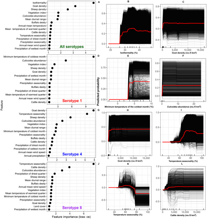
(A, D, G, J) Plots showing feature importance (i.e., environmental and demographic predictors) that contribute to BTV risk in Europe. We used a classification error loss function (loss: ce) to calculate the relative importance of each feature. (B, C, E, F, H, I, K, L) Centered individual conditional expectation (ICE) plots for the top two important features that contribute to BTV risk in Europe. The plots show the relationship between the predicted spatial risk of BTV and each corresponding feature. The black lines indicate the predicted risk of a BTV outbreak in a given geographical site, while the red line indicates the partial dependence calculated as the average risk across all geographic locations in Europe. Panels A–C indicate all serotypes. Panels D–F indicate serotype 1. Panels G–I indicate serotype 4. Panels J–L indicate serotype 8.

Fig. 3.

Feature interaction plots calculated by Friedman’s H statistic. (A–C) indicate all BTV outbreaks; (D–F) indicate serotype 1; (G–I) indicate serotype 4; (J–L) indicate serotype 8. The four plots on the left (A, D, G, J) show overall interaction strength of features with the other features. Plots in the middle (B, E, H, K) demonstrate the overall interaction strength of a single selected feature with the other features. Partial dependence plots on the right (C, F, I, L) represent the top individual interactions between two selected features that shaped the spatial risk of BTV outbreaks. The heat matrix corresponds to the magnitude of spatial risk, in which lighter shades of red indicate low risks, and darker shades of reds indicate high risks. The bar on the right indicates (y hat) the relative risk of an outbreak occurrence with all other feature combinations marginalized.

Fig. 4.

Feature value contributions for each respective bluetongue outbreak based on Shapley values (phi) for eight individual geographical sites across Europe. Positive phi values indicate that this feature increased the risk of a given BTV outbreak. Negative values indicate that the predictor lowered the risk of a BTV outbreak emerging at a particular geographical site. The numbers next to the features’ names indicate the observed value of that feature for that specific site. (A, B) BTV positive and negative sites for all serotypes, (C, D) for serotype 1, (E, F) for serotype 4, and (G, H) for serotype 8. All sites observed and predicted, either positive or negative.

The minimum temperature of the coldest month followed by midge abundance were the most important predictors of serotype 1 outbreaks in Europe (Fig. 2D). The marked increase in risk of observing serotype 1 outbreaks in locations where a threshold in the minimum temperature of coldest month is above 3°C and at least 1 species of midges observed per 5 km² (Fig. 2E,F). In each case, risk plateaued at values higher than these thresholds. The vegetation index, followed by the minimum temperature of the coldest month, also had the strongest overall interactions with other features (Fig. 3D). For example, the strongest interaction was between mean temperature of warmest quarter and vegetation index (Fig. 3E). Higher and moderate vegetation indices (NDVIs between 100 and 243) and temperatures ranging 10°–25°C increased the risk of BTV outbreaks (Fig. 3D). A serotype 1 outbreak was likely observed in southern Italy due to increased temperature in the coldest month in areas with moderate vegetation indices ($\cong$145 NDVI and $\cong$3°C, respectively; Fig. 4C). However, a serotype 1 outbreak was likely absent in northern Denmark due to temperatures of <−12°C, and low sheep density (<215 animals/5 km²; Fig. 4D).

In contrast, goat density followed by temperature seasonality were the most important predictors of serotype four outbreaks (Fig. 2G). Risk of a serotype 4 outbreak increased rapidly at low goat density (>500 animals/5 km²) and high (>65%) seasonality before plateauing (Fig. 2H, I). Sheep density, followed by temperature seasonality, had the strongest overall interactions with other predictors (Fig. 3G). Like the all BTV outbreaks model, the strongest interaction was between sheep and goat density using serotype 4 model (Fig. 3H,I). Shapely values revealed that serotype 4 outbreak likely observed in southern Greece was mainly due to marked and small increases in precipitation seasonality and mean diurnal range, respectively (>77% and >11°C, Fig. 4E). Conversely, in southern Sweden, a serotype 4 outbreak was likely absent due to decreases in sheep density and minimum temperature of the coldest month (<199 animals/5 km² and <−9°C, Fig. 4F).

Finally, temperature seasonality and cattle density were the most important features for predicting serotype 8 outbreaks (Fig. 2J). Moderate temperature seasonality ($\cong$50%) increased the risk of serotype 8 outbreaks, while increased temperature variation throughout the year decreased (>70%) the risk of observing serotype 8 outbreaks (Fig. 2K). Additionally, slight rises in cattle density increased the risk of serotype 8 outbreaks (Fig. 2L). Precipitation of the driest quarter, followed by precipitation and temperature seasonality, had the strongest overall interactions with other predictors (Fig. 3J). Increased precipitation during the driest months accompanied by small increases in cattle density elevated the risk of serotype 8 outbreaks (Fig. 3K, L). A serotype 8 outbreak likely observed in central France due to shallow and moderate increases in the abundance of midges and temperature seasonality (>4 species observed per 5 km² and >60%; Fig. 4G). Conversely, a site in southern France was likely negative for serotype 8 outbreaks due to substantial declines in cattle density and absence of midges (<326 animals/5 km² and 0 species observed/5 km²; Fig. 4H).

Discussion

Using an integrated ML pipeline and two decades of outbreak data, we uncovered new insights into the spatial epidemiology of BTV as well as the unique host and landscape contributions to outbreak risk in Europe. Overall, we found that host density coupled with temperature were the most important variables shaping outbreak risk, with vector abundance and precipitation of less predictive value. Importantly, the combination of host and temperature variables shaping outbreak risk was unique for each subtype. Our models had high predictive performance without including temporal information revealing that over smaller timescales (19 yr) host and climate variables are sufficient for predicting BTV outbreak risk. These insights not only inform risk‐based surveillance efforts in Europe but assist with reducing the economic implications of this important animal pathogen. Moreover, similar nonlinear interactions between host species and environment are likely important for predicting risk of other vector‐borne pathogens and we demonstrate the utility of our interpretable machine learning in quantifying this complexity.

Temperature variation, vector abundance, and host densities are critical components for the maintenance and circulation of all BTV serotypes in Europe. Our findings are in agreement with Samy and Peterson (2016) that found high suitability of the environmental conditions in southern European countries across the Mediterranean Basin for the spread and maintenance of BTVs (Fig. 1). However, we demonstrate that the specific combination of host and environmental factors that shaped outbreak risk was strongly serotype‐specific. Other epidemiological characteristics are likely to vary by serotype as well. For example, serotype‐level differences have also been detected in the rate of spread of serotypes 1, 4, and 8 (Nicolas et al. 2018). Similarly, the environmental determinants of spread also have a unique serotype signature (Nicolas et al. 2018). For genetically diverse pathogens, serotype or subtype may be the more appropriate and meaningful taxonomic units for epidemiological investigation as it is in other systems (e.g., Fountain‐Jones et al. 2017). However, our models did not include the effect of past and present vaccination campaigns in changing the risk out BTV serotype outbreaks. Vaccination did slow down the spread of serotype 1 in France during the 2008 epidemic (Pioz et al. 2012). Yet, the role of the environmental factors in predicting the rate of BTV spread was important for evaluating the effectiveness of vaccination activities (Pioz et al. 2012). Hence, our serotype‐specific outbreak models could be used to set risk‐based vaccination zones. Future work should focus on assessing the role vaccination in shaping the outbreak risk of each highly prevalent serotype. Further, while our models utilized the best data on midge diversity possible at this scale, high resolution estimates of midge species abundance, while difficult to collect, will likely provide more nuanced estimates of serotype outbreak risk.

While we did not have direct measures of midge density, we found that temperature variations that are likely proxy for vector behavior and density played a dominant and complex role in shaping the serotype outbreak risk (Figs. 2, 3, 4). We show that there is no linear increase risk in BTV outbreaks with increased temperature, and each serotype was predicted by variables related to temperature in distinctive ways. Our findings do not support that a general increase in temperature makes BTV outbreaks more likely (Turner et al. 2012). In contrast, our c‐ICE plots (Fig. 2B, E, I, and K) and feature interaction (Fig. 3) plots show that the relationship between temperature derivatives and BTV occurrences is nonlinear and far more complex (Napp et al. 2016, Jacquot et al. 2017). For example, larger or smaller temperature fluctuations within a month relative to the year as well as over the course of the year maintain BTV circulation and emergence (Brand and Keeling 2017). While there is a common notion that mean temperatures of 20°–25°C (Wittmann et al. 2002, Maclachlan 2010) is the threshold for BTV outbreaks, our results suggest that the occurrences of different BTV serotypes require different thresholds of temperature fluctuations (Fig. 2B, E, I, and K). Mean temperature alone seems not to be the sole risk factor for an outbreak and this is supported by other models of BTV outbreak risk (Nicolas et al. 2018). Finer resolution spatiotemporal models including, for example, weekly climate data may enhance our understanding of outbreaks and enhance outbreak predictive capacity.

Unlike temperature, precipitation was not as important in shaping the outbreak risk of all BTV serotypes (Fig. 1). However, precipitation seems to have a more complex role in terms of the strength of interactions with other ecological and environmental features (Fig. 3), particularly for serotype 8 (Fig. 3K). The link between precipitation and other environmental factors has been documented previously (Pioz et al. 2012). For example, heavy precipitation accompanied by extreme temperature events occurred before the emergence of serotype 8 in France between 2007 and 2008 (Pioz et al. 2012). We provide more nuance to this observation and show that precipitation of the driest month coupled with cattle density shape serotype 8 outbreak risk (3L). The ability of our ML pipeline to identify these biologically plausible nonlinear interaction thresholds shows the utility of this approach. Our results also indicate that it requires only a few species of Culicoides to be observed in a given geographical location for it to be a high‐risk area for BTV (Figs. 2I, 4A–D). This finding agrees with past studies in implicating specific species in spreading notable BTV outbreaks across Europe (Kiehl et al. 2009, Cuellar et al. 2018).

Our results were consistent with past studies in terms of the critical role of livestock densities in shaping the risk of BTV in Europe (Breiman 2001, Jacquot et al. 2017). We revealed that not just sheep and cattle were important predictors of BTV outbreaks overall, but also goat and buffalo densities also played a role (Figs. 2, 3). For example, we found that for serotype 4, if goat density was low, the risk of outbreaks was low even if sheep density was high (Fig. 3). However, a limitation of our approach is that our BTV absences may have occurred in areas with no suitable hosts. Future work on developing techniques to select locations of absences weighted by host density may address this limitation. While past studies were inconclusive about the role of goats in maintaining BTV infections, they have always been recognized as major hosts for BTV worldwide (Hofmann et al. 2008, Zientara et al. 2014, Savini et al. 2017, Alkhamis et al. 2020). The extended period of viremia of BTV infections and the unapparent clinical signs in goats (Coetzee et al. 2012, Vogtlin et al. 2013) makes this species an ideal reservoir by providing the ideal conditions for continuous emergence and re‐emergence of new strains (Savini et al. 2017). Furthermore, goat density was found to be positively associated with the evolution and spread of BTVs in Europe (Jacquot et al. 2017). Therefore, restricting goat movements and mixing with other livestock, as well as intensifying surveillance activities on their populations during emerging BTV epidemics, could substantially help improve control and prevention efforts. The complexity of BTV epidemiology, coupled with the increasing size of the data as well as highly nonlinear host and environmental relationships highlight the strengths of our ML approach. The ML algorithms integrated into our pipeline were shown to outperform simpler and commonly used algorithms such as logistic regression (Fountain‐Jones et al. 2019) and maximum entropy models (Mi et al. 2017). Further, we demonstrate the utility of Shapley values to explain in finer scales what each model means in terms of spatial risk of different BTV serotypes. This intuitive property can be used to guide decision‐makers and intervention activities. For example, at the randomly selected site in central France (Fig. 4G), specific thresholds of midge abundance, cattle density, and temperature made that site at high risk for a serotype 8 incursion. In contrast, the other selected site in southern France (Fig. 4H) completely lacks such thresholds. Therefore, a site in central France should be targeted as a priority for surveillance and vaccination activities.

Further application of our ML pipeline to guide policymakers in their intervention activities will help to reduce the economic implications of BTV outbreaks in Europe and provide a blueprint for other regions of the world impacted by this economically damaging virus. More broadly, our pipeline offers a powerful way to merge high dimensional host, vector, and environment data to build complex but interpretable predictive models of outbreak risk down to serotype level. Application of similar approaches can guide not only pathogen surveillance but also provide valuable insights into the ecological determinants of outbreak risk for vector‐borne pathogens.

Supporting information

Appendix S1

Alkhamis, M. A. , Fountain‐Jones N. M., Aguilar‐Vega C., and Sánchez‐Vizcaíno J. M.. 2021. Environment, vector, or host? Using machine learning to untangle the mechanisms driving arbovirus outbreaks. Ecological Applications 31(7):e02407. 10.1002/eap.2407

Open Research

All data and code (Alkhamis et al. 2021) are available on Zenodo: https://doi.org/10.5281/zenodo.5076620.

Literature Cited

- Alkhamis, M. A. , Aguilar‐Vega C., Fountain‐Jones N. M., Lin K., Perez A. M., and Sánchez‐Vizcaíno J. M.. 2020. Global emergence and evolutionary dynamics of bluetongue virus. Scientific Reports 10, 21677. [DOI] [PMC free article] [PubMed] [Google Scholar]