Characterizing the Response of Vegetation Cover to Water Limitation in Africa Using Geostationary Satellites

Abstract

Hydrological interactions between vegetation, soil, and topography are complex, and heterogeneous in semi‐arid landscapes. This along with data scarcity poses challenges for large‐scale modeling of vegetation‐water interactions. Here, we exploit metrics derived from daily Meteosat data over Africa at ca. 5 km spatial resolution for ecohydrological analysis. Their spatial patterns are based on Fractional Vegetation Cover (FVC) time series and emphasize limiting conditions of the seasonal wet to dry transition: the minimum and maximum FVC of temporal record, the FVC decay rate and the FVC integral over the decay period. We investigate the relevance of these metrics for large scale ecohydrological studies by assessing their co‐variation with soil moisture, and with topographic, soil, and vegetation factors. Consistent with our initial hypothesis, FVC minimum and maximum increase with soil moisture, while the FVC integral and decay rate peak at intermediate soil moisture. We find evidence for the relevance of topographic moisture variations in arid regions, which, counter‐intuitively, is detectable in the maximum but not in the minimum FVC. We find no clear evidence for wide‐spread occurrence of the “inverse texture effect” on FVC. The FVC integral over the decay period correlates with independent data sets of plant water storage capacity or rooting depth while correlations increase with aridity. In arid regions, the FVC decay rate decreases with canopy height and tree cover fraction as expected for ecosystems with a more conservative water‐use strategy. Thus, our observation‐based products have large potential for better understanding complex vegetation‐water interactions from regional to continental scales.

Key Points

• We derive ecohydrological metrics from seasonal decays in geostationary satellite data of vegetation cover over Africa at 5 km resolution

• The metrics covary with soil moisture, contain information on water sources apart from precipitation and vegetation access by deep rooting

• Land surface models can benefit from these metrics by tailored evaluation, calibration, and parameterization of ecohydrological processes

1. Introduction

Africa hosts the largest share of undernourished population, and the livelihood of the majority of its population relies on ecosystem services and water availability (Müller et al., 2014). Moreover, African ecosystems contribute strongly to fluctuations of the global carbon cycle (Palmer et al., 2019; Valentini et al., 2014; Weber et al., 2009; Williams et al., 2007). However, large uncertainties prevail in understanding the African ecosystems and quantifying spatiotemporal variations of their functioning due to the complexity of continental gradient and scarcity of ground measurements. This has been shown in studies using different data and approaches ranging from in‐situ observations (Schmiedel et al., 2021), over remote sensing (Weerasinghe et al., 2020), to ecosystem modeling (C. Martens et al., 2021), as well as systematic literature reviews (Adole et al., 2016).

Savannas cover majority of the African continent (Williams & Albertson, 2004), and water is the limiting factor in such ecosystems, affecting vegetation's carbon uptake and nitrogen assimilation (Rodríguez‐Iturbe et al., 1999). The dominant role of water in African drylands has been shown in various studies (Merbold et al., 2009; Sankaran et al., 2005, 2008; F. Wei et al., 2019). Moreover, evidence suggests that ecosystem functioning—even in the wettest part of the continent, the central African tropical forest—responds to soil moisture fluctuations (Gond et al., 2013; Guan et al., 2013) along with co‐limitations of other factors such as radiation (Adole et al., 2019). Within the complex rainfall seasonality patterns having unimodal, bimodal or trimodal regimes, less than 5% of the continent is reported to be non‐seasonally humid (Herrmann & Mohr, 2011).

Soil moisture is the critical variable that characterizes the water limitation of vegetation (Porporato et al., 2001), which, in turn, shapes land‐atmosphere exchanges of carbon, water, and energy fluxes (Gentine et al., 2012), phenology (Peñuelas et al., 2004), and vegetation functional traits (Guan et al., 2015; W. Zhang et al., 2019), along with their species or biome distribution (Xu et al., 2016). Rainfall is the primary source of moisture but plant available water in drylands is characterized by non‐trivial and complex ecohydrological processes that control the availability of moisture from secondary sources (D’Odorico et al., 2019). Overall, comprehensive understanding on multiple ecohydrological processes is needed to understand land‐atmosphere interactions under water limitation.

In order to address this problem in a systematic way, Wilcox et al. (2017) conceptualized three critical ecohydrological junctures: (a) infiltration versus overland flow, (b) soil evaporation versus transpiration, and (c) root water uptake versus drainage, that are all centered around the hydrological response of the ecosystem. Beyond precipitation intensity, topography, and soil properties, the first juncture is affected by presence of vegetation patches that interact with overland flow causing the typical runoff‐runon dynamics at hillslope‐scale (Ludwig et al., 2005). The second juncture, partitioning of terrestrial evaporation, is critical as an interplay between biological activity and productivity, and physical water losses by direct evaporation. Vegetation transpiration generally dominates terrestrial evaporation (Z. Wei et al., 2017), and the partitioning is controlled more by vegetation and soil characteristics given the climate (Nelson et al., 2020), highlighting a pivotal role of vegetation. The third juncture within the root zone is largely controlled by below‐ground vegetation properties, such as depth and distribution of roots, that control the soil‐plant hydraulics continuum. Deep rooting facilitates access to a larger moisture reservoir, a frequently observed trait in savanna and woodland ecosystems (Guswa, 2008; Kleidon & Heimann, 1998). In fact, the diversity and complementarity of ecohydrological plant traits by different species within ecosystems was shown to determine resilience to drought (Anderegg et al., 2018) and to maximize plant water use (Caylor et al., 2009; Scanlon et al., 2005).

There are further ecohydrological phenomena that should be considered when exploring vegetation‐water interactions, emerging from non‐monotonic ecosystem responses to episodic events, and ephemeral waterbodies occurring across spatial scales. Non‐monotonic effects of soil properties on the interaction between climatological aridity and vegetation can lead to the frequently observed “inverse texture effect” in arid climates, whereby sandy soils appear to be associated with less water stress compared to clay soils, due to their higher infiltration capacity (Noy‐Meir, 1973). Additionally, dryland ecosystems locally return nearly all rainfall back to atmosphere as terrestrial evaporation (Newman et al., 2006) with very little water draining from the root zone to groundwater (Wilcox et al., 2017), except extreme rainfall events that episodically recharge aquifers (Taylor et al., 2013; J. Zhang et al., 2016). Moreover, riparian processes such as river channel losses from ephemeral rivers can provide critical source of moisture (Jacobson & Jacobson, 2013; Mansell & Hussey, 2005; Tooth, 2000; Wang et al., 2018). Riparian corridors and groundwater‐fed valleys, therefore, often appear as “green islands” (Eamus et al., 2015), where access to the shallow groundwater supports vegetation activities. In such ecosystems, the growing season may continue several months after the rain season has ceased while the trees appear to have access to groundwater via deep roots or recharge their trunks with water during these times (Guan, Wood, et al., 2014; F. Tian et al., 2018).

Previous studies, therefore, provide clear evidence that vegetation functions are controlled by moisture availability in non‐humid climate, with moisture availability, itself, emerging from the complex interplay among climate characteristics, vegetation traits, hillslope topography, soil properties, and presence of secondary moisture sources, for example, aquifers. In fact, incorporation of all these ecohydrological factors poses a challenge for land‐surface modelers (Clark et al., 2015; Fisher & Koven, 2020). Relatedly, models overestimate sensitivity between ecosystem productivity and precipitation in annual scales, which increases uncertainty in climate models against drought conditions (Ukkola et al., 2021). Moreover, disagreements within models become larger with stronger water limitation, where parametrization of plant water stress is non‐standard and often ignores soil texture properties (Paschalis et al., 2020). Consequently, models fall short on capturing ecosystem exchange in annual and interannual time scales (MacBean et al., 2021), where authors suggest improvements in simulating vegetation responses to changes in water availability. Another main limitation for models is the specification of Rooting Depth (RD) (Fan et al., 2019). Over recent years, several studies have put forward estimations of the rooting depth or Effective Rooting Depth (ERD) that represents the potential moisture access of the vegetation. A comparison of different estimates, though, reveals a large uncertainty with rooting depth varying from a few centimeters to tens of meters for a given location (Wang‐Erlandsson et al., 2016). This, in part, is caused by the underlying assumptions in the estimation methods, whose effect on the prediction cannot be constrained by or validated against observations, especially in data scarce regions like Africa. Considering the particular difficulties associated with below‐ground observation of ecosystem and land properties at large‐scales, remotely sensed products of vegetation characteristics, indices, and responses provide opportunities to back infer the underlying environmental factors and land surface characteristics.

Remote sensing vegetation indices has been extensively used to capture phenological states of vegetation, such as detecting onset and length of growing season or peak greenness, as well as specific agricultural applications (reviewed in Zeng et al. [2020]). Moreover, the temporal dynamics of vegetation indices can be exploited to understand ecologically relevant concepts such as land cover effects on vegetation dynamics (Yan et al., 2017), early green‐up of woody vegetation in Africa (Adole et al., 2019; Guan, Wood, et al., 2014; Ouédraogo et al., 2020), effects of plant water storage (F. Tian et al., 2018), and early diagnosis of climate‐induced forest mortality (Liu et al., 2019). The majority of vegetation remote sensing studies focusing on Africa are based on image acquisitions from polar orbiting satellites like MODIS (Adole et al., 2016), while only a few studies are based on vegetation indices derived from the geostationary satellite Meteosat Second Generation (MSG; e.g., Guan, Medvigy, et al., 2014; Yan et al., 2017). Geostationary satellite based vegetation indices are available in daily temporal resolution, which is their biggest advantage compared to polar orbiting satellites where such high resolution in time is not possible.

In this study, we analyze the daily Fraction of Vegetation Cover (FVC) time series from MSG to infer the ecohydrological characteristics of ecosystems over Africa. We derive a set of ecohydrological metrics from the vegetation decay period, and evaluate their spatial patterns. Our overarching hypothesis is that these metrics, derived from the vegetation dynamics over decay periods, contain valuable information on plant water access, presence of secondary moisture sources, and other ecohydrological processes, which are modulated by climate, topography, soil properties, groundwater access, as well as vegetation traits and scales. The ecohydrological metrics include (a) robust estimates of the minimum and maximum FVC, (b) FVC integral over the decay period, and (c) the exponential decay rate during dry‐down. Using the metrics, we evaluate several hypotheses that encompass the ecohydrological characteristics of moisture‐limited ecosystems and the influence of environmental factors and land characteristics therein, such as:

1. In arid regions, minimum and maximum FVC are larger in sandy soil while this covariation is inverted in semi‐arid and humid regions. This hypothesis follows the “inverse texture effect” (Noy‐Meir, 1973) often reported in drylands.

2. Within similar climatic aridity, secondary moisture sources increase the minimum FVC and decrease seasonal FVC range. This hypothesis is derived from the classical approach of mapping groundwater‐dependent ecosystems—with shallow water table or potentially larger runoff due to topography—as “green islands” of attenuated seasonality (Eamus et al., 2015).

3. The time integral of FVC over the decay period as a proxy for plant accessible water storage is larger in semi‐arid regions where the water deficit (the difference between precipitation and potential transpiration) is marginally smaller at annual scales than at seasonal scales, compared to arid regions. This hypothesis follows the theory that vegetation expands root zone storage capacity to compensate water deficit during dry season (Wang‐Erlandsson et al., 2016), parallel to the expected optimal RD of plants considering cost and benefit of developing root structure (Guswa, 2010).

4. FVC decay rate driven by progressive water limitation becomes lower with increasing aridity, tree cover and canopy height. This hypothesis assumes FVC mimics the decay rate of land evaporation during decay period and follows previously reported increase in timescale of land evaporation decay with aridity, canopy height, and woody vegetation (Boese et al., 2019; Martínez‐de la Torre et al., 2019; Teuling et al., 2006). Therefore, FVC decay rate would reflect adaptations of ecosystem water use strategies.

We approach the analysis first by looking at the continental scale variations of the metrics, together with climatic aridity as the first order driver. This covariation is further scrutinized with other environmental factors relevant to the hypotheses given above. As aridity metric we chose mean annual root‐zone soil moisture from the Global Land Evaporation Amsterdam Model (GLEAM).

To derive the ecohydrological metrics for the African continent from high‐resolution remote sensing data (Section 2), we developed a robust methodology (Section 3) to deal with noise, gaps, widely varying dynamics, and data size. The quality diagnostics along with the derived metrics and discussion of underlying mechanisms (Section 4), and open code for derivations, enables future advances in understanding and modeling ecohydrological processes and variability. Furthermore, initial analysis and corroboration with independent data illustrates the potential of applications of the ecohydrological metrics (Section 4). Finally, we close the manuscript with a summary of the study and potential outlook (Section 5).

2. Data

2.1. Fraction of Vegetation Cover

The FVC, derived from a spectral mixture analysis of the satellite retrievals, is a vegetation index summarizing the two‐dimensional coverage ratio of vegetation per unit land area (Trigo et al., 2011). With a range of [0–1], FVC is often used to derive fundamental vegetation indices such as the Leaf Area Index. The FVC product used in this study, officially labeled as LSA‐421 (MDFVC), was obtained from the Satellite Application Facility for Land Surface Analysis (LSA‐SAF) of the European Organization for the Exploitation of Meteorological Satellites (EUMETSAT). The product is based on the retrievals of the Spinning Enhanced Visible and Infrared Imager (SEVIRI) sensor on board the MSG satellite (Trigo et al., 2011). As a geostationary satellite, the MSG has a circular spatial coverage of Earth centered at 0° longitude, and it covers Europe and Africa entirely (see an example of the original FVC data for a day in Figure A1). The SEVIRI is a multispectral optical sensor with 12 spectral bands, and a temporal resolution of 15 min. Under the sub‐satellite point (nadir), it has 3.1 km spatial resolution in the normal bands, and a high‐resolution band with 1 km spatial resolution. The spatial resolution of the retrieval decreases with increasing distance from nadir.

The FVC data product is available at daily temporal resolution spanning the time period from early 2004 to present. FVC is estimated using parameters of a bidirectional reflectance distribution function on the cloud‐corrected top of canopy reflectance values of three spectral channels namely red, near‐infrared, and middle‐infrared (García‐Haro et al., 2019; LSA‐SAF, 2016). Thanks to the very high temporal resolution of the SEVIRI sensor, spatial consistency of cloud‐free data is ensured by the data providers (Trigo et al., 2011), which is also confirmed by studies comparing enhanced vegetation index products of SEVIRI and MODIS across the Congo Basin (Yan et al., 2016). Further details of the product, and access to downloading data are available at https://landsaf.ipma.pt/en/products/vegetation/fvc/.

For this study, we selected the spatial domain as the African continent. In order to convert the product into equal width grids to facilitate analyses with other products, we resampled the original data to a spatial resolution of 0.0417° (ca. 5 km) via nearest neighbor (using gdalwarp function in GDAL, GDAL/OGR contributors, 2020). In terms of temporal domain, we used nearly 16 years of data, from the beginning of the records in 2004, to the end of 2019.

2.2. Ancillary Data

2.2.1. Soil Moisture

We used the third version of GLEAM estimates of root‐zone soil moisture (B. Martens et al., 2017; Miralles et al., 2011). GLEAM consists a set of modules to estimate different components of land evaporation simultaneously. Therefore, the model estimates multiple products including root‐zone soil moisture (hereafter referred to as soil moisture). Among the input data of the model, precipitation may have relatively low quality over Africa due to lower density of rain gauges across the continent. However, the model assimilates satellite based soil moisture, which is known to be of the best quality in semi‐arid regions with sparse vegetation. GLEAM data is available at 0.25° space and at daily resolution in time from 2003 up to date with a small latency. We used mean value of daily estimates from 2004 to 2019 (parallel to the temporal domain of FVC data used) as a diagnostic for average climatological aridity in Section 4. Additionally, we used daily values to compute temporal correlation between soil moisture and FVC, after aggregating original FVC data into 0.25° by simple averaging (see Appendix D for spatial variation of correlation values).

2.2.2. Sand Content of Soil

In order to quantify effects of soil texture, we used gridded sand percentage of soil data from SoilGrids data set (Hengl et al., 2017), which is a machine learning based interpolation of soil profiles at 250 m resolution. SoilGrids data set is available globally and provides information from different layers, ranging from surface to 2 m depth. Though in this study, for interpretability, we used the average of the top five layers that are not deeper than 1 m for interpretability, and used the data at 0.0417° after aggregating by simple averaging.

2.2.3. Height Above Nearest Drainage

To relate the variation of the metrics to meso‐scale heterogeneity and convergence of moisture caused by topography, we used the Height Above Nearest Drainage (HAND) data from Yamazaki et al. (2019). Quantifying the vertical distance of a given point to the nearest drainage, HAND is closely related to drainage topology and hillslope‐scale convergence of soil moisture and groundwater (Nobre et al., 2011). The HAND data used here is based on the MERIT digital elevation model at a spatial resolution of 3‐arc second (ca. 90 m). We used the original high‐resolution data after aggregating (simple average) to the resolution of the ecohydrological metrics presented in this study (0.0417°).

2.2.4. Topographic Wetness Index

In order to understand the runoff related effects of topography, we used Topographic Wetness Index (TWI), also known as compound topographic index. Being a function of both slope and the upstream area that potentially contribute to runoff of a given point, TWI is a metric to diagnose topography‐induced effects on water cycle at hillslope scales. Even though HAND and TWI are both topography related metrics, TWI, being a function of upstream area and slope of a given point, is a proxy for runoff, while HAND is a proxy for water table depth. We used TWI data from Amatulli et al. (2020), which is computed by using the MERIT digital elevation model at 3‐arc seconds, as in the case of HAND. In order to account for the high variability of TWI at hillslope scales while aggregating the data into 0.041 7°, we first calculated median TWI value of the domain (0.069). Then, we aggregated the TWI values by calculating percentage of sub‐grid cells having larger TWI values than the median value computed in the first step. Eventually, similar to TWI itself, larger values in the normalized TWI means larger potential runoff due to topographic complexity.

2.2.5. Accessible Water Storage Capacity and Rooting Depth

We used multiple proxies of plant accessible water to understand their effects on vegetation dynamics. Effective RD (ERD, Yang et al., 2016) is one of those products, which is natively at 0.5° spatial resolution. ERD comes from a global parametrization of a process‐based, analytical model of carbon costs and benefits of deeper rooting in plants, proposed by Guswa (2008). In this model, the cost of deeper roots is estimated considering the physical structure of roots like density and length together with root respiration, while the benefit is estimated considering water use efficiency, growing season length and mean transpiration rate per rooting depth. In order to parametrize the model, root and soil properties were obtained from the literature, water use efficiency from an ensemble of process based models while climatological information from a long‐term mean of remote sensing based products.

In addition, the RD product from Fan et al. (2017) is also used in this study. RD is estimated with inverse modeling of root water uptake profiles in three steps, where first soil water profile, as the supply, is estimated using climate, soil properties and topography. Thanks to the availability of high‐resolution information on soil and topography, RD has a much higher spatial resolution (0.0083°, ca. 1 km) than the other products. After estimation of plant water demand using atmospheric conditions and leaf area index, the supply is allocated as root water uptake using Ohm's law at different soil depths, where amount of infiltration, groundwater recharge, and subsequent uptake were effected (Fan et al., 2017). Note that the model includes multiple forcing data, with a temporal coverage from 1979 to the time of the study.

Apart from the rooting depth products, we also used estimates of plant water storage capacity. Accessible Water Storage Capacity (AWSC, S. Tian et al., 2019) is derived at 0.25° by assimilating an ecohydrological model (World‐Wide Water, van Dijk et al., 2013) with different remote sensing based water observations, namely surface water extent, near‐surface soil moisture and variations of terrestrial water storage. World‐Wide Water is a process based model using atmospheric conditions, containing three soil layers to simulate vegetation access to soil moisture, which also accounts for recharge and discharge from groundwater. Due to the temporal availability of the forcing data, AWSC product is derived using 6 years of data starting from 2010.

The forth and last product used to analyze plant AWSC is the Root Zone Storage capacity (RZS _CRU2, Wang‐Erlandsson et al., 2016) product derived by contrasting water fluxes observed by remote sensing, precipitation and irrigation as influx, and evaporation as outflux. Owing the assumption that plants develop their roots to optimize their root zone storage capacity, and using a simple approach on water fluxes, Wang‐Erlandsson et al. (2016) did not use any external information on vegetation or soil properties. While different precipitation data are used as forcing data with different drought return periods, we used the final product forced by Climate Research Unit precipitation data (CRU TS3.22, Harris et al., 2014) with the shortest return period, 2 years. RZS _CRU2, which is derived using data from 2003 to 2013, is available at 0.5° spatial resolution.

For a consistent comparison across data at different resolutions, we aggregated all data to a common spatial resolution of 0.5° by simple averaging. Note that the spatial aggregation may result in loss of the spatial variability prevalent locally and potentially captured at a high resolution. Moreover, we only used the grid cells that all products have an estimate.

2.2.6. Canopy Height

Since canopy height is an important indicator of ecosystem functions and is associated mostly with water limitation (Tao et al., 2016), we analyzed the effects of canopy height on the decay rate of vegetation cover through their covariation in space. We used the lidar‐derived canopy height data from the retrievals of the ICESAT satellite at a spatial resolution of 1 km (Simard et al., 2011). We used the data after aggregating (simple average) to 0.0417°.

2.2.7. Tree Cover

We used tree cover data in order to analyze the sensitivity between the relationship of decay rate of FVC and climatological aridity. We used the tree percent component of the MOD44B Version 6 Vegetation Continuous Fields from MODIS (Dimiceli et al., 2015), which is available globally in 250 m spatial and annual temporal resolution. We aggregated the product in space to the target resolution of this study by taking the mean of higher resolution grid cells. Finally, we used the median tree cover value over the years covering the temporal domain of FVC data to obtain a time invariant metric, same approach taken for the annual estimates of the metrics derived from FVC (see Section 3).

3. Methodology

The derivation of the ecohydrological metrics is based exclusively on the daily FVC time series. The method can be divided into four main steps: (a) masking and retrieval of minimum and maximum FVC (FVC_min and FVC_max), (b) detection of start and end of the decay periods, (c) estimation of the decay period FVC integral (I _dp ), and (d) estimation of the FVC decay rate during dry‐down (λ). Each methodological step is described in detail in the following subsections together with the final products, and their quality diagnostics when needed.

3.1. Masking and Retrieval of FVC Extrema

To remove the effect of outliers within a time series, we selected the 2nd and 98th percentiles of the entire records of the FVC data as the minimum (FVC_min) and the maximum asymptotic values (FVC_max). To maintain a reliable signal‐to‐noise ratio before taking further steps, we filtered out any grid cell if FVC_max < 0.1 or more than one‐third of the time series were missing. Due to the simplicity of the derivation of FVC_min and FVC_max metrics, quality diagnostics were deemed unnecessary, and not derived in this set of metrics.

3.2. Detection of Decay Periods

The detection of the decay period was based on a procedure using the first derivative of the smoothed FVC (V′) (see Algorithm 1). We smoothed daily time series of the FVC with a 31‐day moving average (V _sm ). Then each day in the time series was marked as decay, growth or stable. To do so, we set two thresholds for decay and growth periods as th _decay and th _growth, respectively. After rigorous investigation of time series of individual grid cells, we used the 75th and 70th percentiles of the negative derivative (V′) as thresholds th _decay and −th _growth for each grid cell. The magnitude th _decay is, thus, bigger than th _growth, in accordance with the larger gradient in the beginning of the period than the end. Only the magnitude of th _growth was taken as a positive threshold to detect the increase in FVC.

Algorithm 1. Detection of Decay Periods From the Entire Time Series.

1.

1: Smooth FVC time series with 31 days moving average; to yield Vsm

2: Calculate the first derivative of FVC time series from Vsm with daily step size; to yield V′

3: Through the entire time series, set the threshold for decay as thdecay = percentile(V′, 75) where V′ < 0

4: Through the entire time series, set the threshold for growth as thgrowth = −1 × percentile(V′, 70) where V′ < 0

5: Mark each observation for their corresponding period as:

  if V′ < thdecay then decay

  else if V′ > thgrowth then growth

  else stable

6: Smooth the classes with a 5‐day moving window by majority voting

7: Label consecutive observations marked with decay and followed by stable ones as decay period

8: Extend every decay period label until Vsm > min(Vsm) + 0.05 × (max(Vsm) − min(Vsm)) is satisfied in the corresponding season

9: For each grid cell, keep only the longest decay period per year

An observation was considered as decay if V′ < th _decay, growth if V′ > th _growth, and stable if th _decay ≤ V′ ≤ th _growth. The resulting time series of classes (decay, growth, or recovery) were then smoothed by retaining the majority of decay and stable against recovery within a 5‐day moving window. Complete decay period, which is considered as the initial decay period followed by a stable, non‐increasing period, was then identified as the period from the beginning of a decay to the end of a stable period. In order to ensure robustness of the end of the stable period, especially in hyper‐arid regions with poor signal‐to‐noise ratio, we extended the detected decay periods until the next significant increase in V _sm (>5% of the corresponding seasonal amplitude of FVC). Note that selection of the thresholds and the moving window sizes were based on extensive exploration and visual inspection of the FVC time series. This was a necessary step to ensure the robustness against noise in the data, as well to address the diversity of FVC dynamics across African ecosystems. To highlight the complexity, some representative time series of FVC in selected grid cells across different climatological aridity are included in Appendix B, together with soil moisture and precipitation time series.

After detection of all decay periods in the time series, we only selected the longest one per calendar year. This is necessary for regions where vegetation may potentially have two growing (and decaying) seasons within a year. The longest decay period within a year is likely to be the most indicative of the largest water limitation, and the underlying ecohydrological mechanisms. When the detected decay period spanned over two calendar years, it was assigned as the decay period of the starting year. In total, the decay period detection algorithm (Algorithm 1) yielded 16,423,339 decay periods in 1,029,847 grid cells.

3.3. Estimation of the Integral Over FVC Decay

We calculated the integral of FVC during decay period (I _dp ) as the total area under the FVC time series from the start to end of the decay period, with the area under FVC_min removed. This can be expressed as,

$$I_{dp}=\sum ^{decayperiod}\left(FVC(t)-FV{C}_{\min }\right)$$ (1)

Removal of the baseline FVC value (FVC_min) enhances the signal of seasonal decay of vegetation with respect to baseline vegetation activity. Note that, upon necessity, the full integral (total area under the curve) can be calculated as the sum of I _dp and multiplication of decay period duration with minimum FVC (D × FVC_min).

From the yearly dry season detection, 16 (the number of years) values of I _dp were computed for each grid cell. We selected the median of the 16 values as the representative inference to be used for spatial analyses. The median was preferred over the mean to make the estimation robust against annual variations, for instance, by intermittent rain events in the dry season or issues related to FVC derivation. In addition, we also calculate and report the normalized robust Standard Error (SE ) as an indicator of variability. The SE is calculated as,

$$\mathrm{SE}=\frac{{\mathrm{SD}}_n}{\sqrt{n}}$$ (2)

where SD _n is the robust standard error, calculated from the Median Absolute Deviation across years (with the assumption of a normal distribution, Rousseeuw & Croux, 1993), and corrected for the low number of samples (n = 16) as:

$${\mathrm{SD}}_n=MAD\times 1.4826\times \frac{n}{n-1}$$ (3)

The robust standard error reflects variability of the metrics among years as well as methodological uncertainty, and is therefore suitable for customized filtering in the context of spatial analysis.

3.4. Estimation of FVC Decay Rate

Temporal decay of the FVC can be characterized using an exponential function as,

$$FVC(t)=\left(FV{C}_{dd}-FV{C}_{\min }\right)\times e^{-t/\lambda }+FV{C}_{\min }$$ (4)

where FVC _dd is the initial FVC value in the beginning of a dry‐down, and λ is the e‐folding time with the same unit of the time scale (days in our case)—see Figure 1 for a graphical explanation. Note that λ is merely an inverse of the exponential decay rate. The formulation in Equation 4 uses λ as it is easier to interpret. In simple terms, λ denotes the number of days needed to have a decrease in the seasonal amplitude of FVC (FVC _dd  − FVC_min) to 1/e of its original value during a dry‐down event. Note that the selected exponential decay function explicitly takes an asymptotic minimum value of the FVC, as FVC_min, into account while estimating the decay rate (see Section 3.1) since FVC_min is included in the formulation (Equation 4).

Figure 1.

Conceptual plot of the ecohydrological metrics derived from time series using synthetic data. Points represent observations for growing period, early decay period and decay period with dry‐down in light gray, gray and black, respectively. Decay and growth periods are defined by presence of decay, that is, first derivative of the time series, while dry‐down period is defined by the convexity of the decay, that is, using both first and second derivatives (see Section 3.4 for details). The shaded area shows the integral of FVC during decay period. The red curve shows the fitted line on the FVC time series during dry‐down using the asymptotic exponential decay function. All metrics presented in this study are shown in bold characters.

Due to the S‐shaped character of temporal vegetation dynamics, functions allowing different convexity, for example, logistic functions, have been used to characterize these dynamics (Beck et al., 2006). As exponential decay functions are strictly convex, the concave part of the decay, which is mostly observed in the beginning of the decay period, is not considered for this metric. The latter part of the decay period, with convex curvature (i.e., the first derivative is negative while the second is positive), is labeled as “dry‐down” during the decay period. To define the dry‐down period, we first discarded the time steps with concave observations (negative first and negative second derivative). Afterward, we filtered out the convex observations before the inflection point of the FVC, that mostly associated with low signal‐to‐noise ratio at the beginning of the dry‐down. Once daily observations are marked as convex or concave, we searched for local minimum of V′ in the first third of the dry season, and identified the inflection point as the start of the dry‐down. Note that, in the above process, second derivative of the FVC (V″) was also smoothed with a 31‐day moving window.

This procedure effectively removes observations with concave shape in the dry season, especially at the beginning of an event. For each event, if more than half of the data points showed convexity, we estimated λ, together with FVC _dd , based on an asymptotic regression model that minimizes least squares error with the Levenberg‐Marquardt algorithm (Elzhov et al., 2016; Moré, 1978). We used both the Nash‐Sutcliffe modeling efficiency (NSE; Nash & Sutcliffe, 1970) and the standard error of the model (SE _m ) to assess the estimates of the model fitting. From the multiple λ estimates, only those with successful convergence of the Levenberg‐Marquardt algorithm with NSE >0.5 and SE _m (λ) < 0.5 × λ were accepted, the median of which was taken as the representative final λ for a grid cell.

After defining the final λ, we estimated the variation as done in Section 3.3. Unlike in Section 3.3, the sample size per grid cell (n) may change, as λ estimation may not converge in cases with high noise. We, therefore, also report the number of successful convergences of the Algorithm 2 as an additional quality diagnostic that can be used for filtering λ (mapped in Figure I1).

Algorithm 2. Identification of Dry‐Down Periods and Modeling of the Exponential Decay.

1.

1: Smooth V′ with 31 days moving average; to yield $V_{sm}^{\prime }$

2: Calculate the second derivative of FVC time series from $V_{sm}^{\prime }$ with daily step size; to yield V″

3: Smooth V″ with 31 days moving average; to yield $V_{sm}^{″}$

4: Mark each observation with $V_{sm}^{\prime }<0$ as:

  if $V_{sm}^{″}>0$ then convex

  else concave

5: Ignore convex observations before the inflection point of FVC time series, if there is any

6: Ignore concave observations within the decay period and keep the rest as the dry‐down period

7: Discard any event having more concave observations than convex

8: Use Equation 4 on dry‐down period of the decay period to estimate λ

9: Filter out the estimations with NSE < 0.5 OR SE(λ) > 0.5 × λ

4. Results and Discussion

In this section, we present and discuss the ecohydrological metrics derived in this study. For each metric we show the spatial variation in continental scale by maps along with zoomed inset plots (see Appendix E for further information and visual impression by corresponding Google Earth cut‐outs) to visualize regional variability. Box plots of metrics per mean annual root‐zone soil moisture show first order variations while heatmaps show sensitivity of these first order variations to different parameters addressing the hypotheses given in Section 1 (see Section 2.2 for the details of the data). Here we present the metrics independently, but we summarize their cross‐comparison with a density plot in Figure C1.

4.1. FVC Extremes

Spatial distributions of FVC_min and FVC_max, histograms of the distribution over the full domain, and six zoomed insets focusing on selected regions are shown in Figures 2a and 2b, respectively (see Figure G1 for the seasonal dynamics expressed as FVC_max − FVC_min). At the continental scale, both FVC_min and FVC_max follow the moisture gradient with the highest and the lowest values in humid and arid regions, respectively. Saturation in the increase of FVC_max (Figure 2c) in semi‐arid regions suggests that water does not severely limit the vegetation cover at the peak of the wet season in regions with intermediate to high mean annual soil moisture values (see Figure E1 for map of mean annual root‐zone soil moisture as an indicator of climatological aridity together with Google Earth views of the insets). On the contrary, FVC_min stays low up to intermediate mean annual soil moisture and increases only slightly with it suggesting that water limits FVC severely at the peak of the dry season. Understandably, the largest seasonal ranges in FVC are observed in regions with semi‐arid climate systems.

Figure 2.

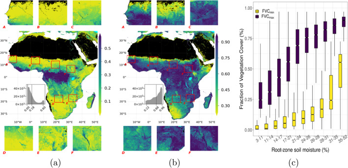
(a) Minimum asymptotic values of FVC, FVC_min, (b) maximum asymptotic values of FVC, FVC_max, and (c) box plot showing the variation of FVC_min and FVC_max with mean annual soil moisture. In the maps, histogram of the metrics mapped can be seen inside the main panel, with a dashed line indicating the mean values of the domain, as well as six insets to show local variability (See Appendix E for details of the insets). In all of the following box plots, binning of soil moisture is done automatically to equalize frequency of observations among the bins while median values per each bin are shown in the intermediate line of the boxes, with their 95% confidence intervals notched. Upper and lower edges of the boxes show the interquartile range (75th and 25th percentiles, respectively) while the error bars show 1.5 times the interquartile range.

In addition to the climate‐associated large‐scale gradients, the metrics also exhibit a substantial meso‐scale heterogeneity. In arid regions, FVC_min is higher in areas closer to perennial water sources, as can be seen near the Senegal and Gambia rivers (Box‐A in Figure 2a). FVC_min is also elevated near large inland deltas and wetlands, that is, the Okavango Delta (McCarthy, 2006) and the Sudd swamp (Tootchi et al., 2019), Box‐D and Box‐F in Figure 2a, respectively, presumably indicating groundwater access by the vegetation in the dry season. Interestingly, the meso‐scale spatial patterns differ remarkably between FVC_min and FVC_max with a tendency of FVC_max showing more spatial structure than FVC_min. This is likely because there is too little water input in the dry season to cause big topographic moisture effects for FVC_min except for the perennial secondary water sources. Thus, such meso‐scale heterogeneity suggests the importance of secondary water sources in moisture‐limited systems, especially on top of the large climate‐driven spatial variations, and highlights the value of FVC_min and FVC_max for ecohydrological studies.

4.1.1. Inverse Texture Effect

Here, we tested if an “inverse texture effect” (Noy‐Meir, 1973) could be observed from 5 km spatial resolution remote sensing FVC data over continental Africa on the variations of FVC_min and FVC_max conditioned on mean annual soil moisture and sand content of soil. In humid regions coarse textured soil is less favorable for vegetation than fine textured soil while in arid regions this pattern is inverted. This inverse texture effect has been documented by several site‐scale studies (Fernandez‐Illescas et al., 2001; Laio et al., 2001; Looney et al., 2012; Sala et al., 1988). Noy‐Meir (1973) suggested this inversion to occur with precipitation values of 300–500 mm/year, although it has also been reported for higher precipitation values (Epstein et al., 1997). The inversion of the texture effect in arid climates is likely due to enhanced infiltration and hydraulic conductivity which reduced soil evaporation losses (Noy‐Meir, 1973) and/or due to reduced water stress thanks to lower matrix potentials of sandy soils (Caylor et al., 2005).

We binned soil moisture and sand percentage values to have equal number of observations in each bin of a given variable. We than calculated the mean of FVC_min or FVC_max per soil moisture bin, and mapped the deviation from these values with changing sand percentage in Figure 3 (see Figure F1 for the heatmaps of raw FVC_min and FVC_max values). Our analysis did not show clear patterns of an inverse texture effect where FVC would be expected to increase with sand content. In the driest regions with the lowest mean annual soil moisture level, FVC_min and FVC_max are slightly elevated for low sand content, consistent with the “normal” texture effect. For intermediate aridity levels, no clear and systematic pattern with sand content can be observed. The temporal scale of the metrics might have hindered observing the inverted texture effect, as Noy‐Meir (1973) considered this effect in the context of rain pulses, which remain effective over days to weeks. Furthermore, spatial resolution and quality of the large‐scale data used in this analysis may not be high enough to observe such localized effects. Despite the sound motivation, it remains for further studies to clarify the extent to which the “inverse texture effect” is significant and can be observed from remote sensing products across large domains.

Figure 3.

Deviation of asymptote‐related metrics from their mean per root‐zone soil moisture bins with changing sand percentage, HAND, and TWI. Note that binning of the continuous variables in x‐ and y‐axes are done automatically to equalize frequency of observations among the bins of a given variable.

4.1.2. Green Islands

Another phenomenon we investigated are the “green islands” patterns where localized moisture availability supports vegetation activity in otherwise dried down conditions by analyzing variations in FVC_min and FVC_max conditioned with soil moisture, HAND and TWI. This approach has been used to detect groundwater dependent ecosystems (Barron et al., 2014; Howard & Merrifield, 2010; Jin et al., 2011; Lv et al., 2013; Münch & Conrad, 2007) or riparian corridors (Akasheh et al., 2008; Everitt & Deloach, 1990; Everitt et al., 1996; Neale, 1997) based on high spatial resolution remote sensing within relatively small regions. Here we analyze if such patterns due to secondary moisture sources are still evident at 5 km resolution and at continental scale by looking at the covariation of FVC_min and FVC_max with HAND and TWI, conditioned on mean aridity (Figure 3). HAND is a hillslope scale proxy for groundwater accessibility (Fan et al., 2019) while TWI, a metric considering local slope together with upstream area, is a strong proxy for topographic soil moisture variations (Raduła et al., 2018). Contrary to our expectations, we did not observe a positive effect of these secondary moisture resources in arid regions on FVC_min (Figure 3a) but instead for FVC_max at high aridity levels (Figure 3b). This implies that shallow water table support vegetation with additional moisture during the growing period as also shown in Koirala et al. (2017) but this effect largely disappears in the dry season since most of the secondary moisture resource is also depleted or not available. This suggests that the effect of secondary moisture sources goes much beyond the frequently studied perennial “green islands” phenomenon and is likely more important in the wet rather than the dry season.

4.2. Integral of FVC Decay

The integral of FVC time series during the decay period, I _dp , is smallest in arid regions, followed by humid regions. The largest I _dp values are observed in regions with intermediate to low aridity (Figure 4a). Median values, as well as variations of I _dp within similar climatology is larger when subject to intermediate aridity (Figure 4c). Uncertainties, which may also be driven by interannual variability to some degree (see Section 3.3 for details), are larger in some of the hyper‐arid regions with low FVC and rare, episodic rainfall (Figure 4b).

Figure 4.

(a) Integral of FVC time series in the decay period, I _dp , (b) variation of I _dp , and (c) distribution of I _dp within mean annual soil moisture. See Figure 2 for plotting details.

At local scales, variations in I _dp emerge as a combined effect of climate and other ecohydrological factors change over hillslope scales, such as proximity to the nearest drainage or occurrences of shallow water table depth. While a sharp aridity gradient in Sahel is clearly seen at Box‐A and Box‐B of Figure 4a, local scale increases in I _dp are also present at riparian zones like Senegal River (Box‐A in Figure 4a). Within similar aridity, I _dp is smaller in seasonally flooding regions like the Sudd swamp (Tootchi et al., 2019), Box‐F in Figure 4a. The highest values of I _dp in the Lower Zambezi bear strong similarity with the rooting depth product presented in Wang‐Erlandsson et al. (2016), and the previously reported seasonal hydrologic buffer (Kuppel et al., 2017) in these regions. This motivates further analysis of I _dp with a plant accessible water storage perspective.

4.2.1. Plant Accessible Water Storage

Here, we tested the third hypothesis of the study by analyzing the agreement between I _dp and other plant accessible water storage products, and presenting the conceptual reasoning behind. Conceptually, plant accessible water storage is related to the vertical distribution of roots, and the water holding capacity of the soil that is determined largely by texture and organic carbon content. The root profile of water‐limited ecosystems appears to adapt to the prevailing hydrologic and soil conditions while being constrained by other ecosystem properties and traits (Fan et al., 2017; Guswa, 2008; Laio et al., 2006; Schenk, 2008; Schenk & Jackson, 2002; van Wijk, 2011). Plant accessible water storage controls the propensity and sensitivity of ecosystems to drought stress in dry periods. Various modeling approaches to infer rooting depth or plant water storage capacity have been proposed (explained in detail in Wang‐Erlandsson et al. [2016]), as it cannot be observed directly but still contains a critical information for global‐scale models (Kleidon & Heimann, 1998).

The integral of FVC during the dry season should be positively correlated with plant accessible water storage of the soil, as larger water storage would facilitate vegetation activity for longer period against water‐limited conditions. The continental‐scale patterns of I _dp (Figure 4a) with the largest values in strongly seasonal semi‐arid savanna systems of both hemispheres are qualitatively consistent with the previous observation‐based analysis (e.g., Schenk & Jackson, 2002) as well as the optimality‐based models (e.g., Kleidon & Heimann, 1998). I _dp declines in hyper‐arid regions like the Sahel, the Somalian desert, Southern Africa, as well as the Congo rainforest. A similar pattern would be expected for optimal rooting depth, which increases in regions with small differences between rainfall and potential evaporation in annual scales but large differences in seasonal scales (Laio et al., 2006; van Wijk, 2011). The inset plots in Figure 4a clearly reveal the landscape scale patterns of I _dp , presumably, due to topography‐driven large variations of moisture. This may reflect enhanced and continued moisture supply due to topographic moisture convergence or shallow water tables along with possible adaptations of rooting depth to these local hydrological conditions (Fan et al., 2017).

We compared I _dp with 4 products related to plant accessible water storage, namely two storage capacity products from Wang‐Erlandsson et al. (2016) and S. Tian et al. (2019), and two rooting depth products from Yang et al. (2016) and Fan et al. (2017) at 0.5° across Africa (see Section 2.2 for product details). As shown in Figure J1, there is qualitative agreement of large values of I _dp with AWSC and RZS _CRU2 in the Miombo woodlands and also, to a lesser extent, in the northern savannas. All three also agree on low values in hyper‐arid regions like the Sahel, the Somalian desert and in Southern Africa. In order to quantify the extent of agreement among the five estimates, we made a pairwise comparison of Spearman's correlation coefficient per climatological aridity via soil moisture (Figure 6a). While the overall low‐to‐moderate correlation values among the products available in the literature demonstrate the scale of the challenge in estimating plant water storage capacity or rooting depth, highest correlation was observed between I _dp and RZS _CRU2. Regardless of the product pairs, correlations decrease with increasing humidity, which is presumably related with other limiting factors than water, such as radiation or nutrients.

Figure 6.

(a) Spearman's correlation coefficients between pairs of products related to plant accessible water content, namely Effective Rooting Depth from Yang et al. (2016), Rooting Depth from Fan et al. (2017), Accessible Water Storage Capacity (AWSC) from S. Tian et al. (2019), Root Zone Storage Capacity (RZS _CRU2) from Wang‐Erlandsson et al. (2016), and integral of FVC during decay period (I _dp ) presented in this study. Black dots indicate significant correlation with ρ > 0.05. (b) Covariation of λ and root‐zone soil moisture with canopy height, and tree cover. Note that binning of soil moisture, canopy height and tree cover are done automatically to equalize frequency of observations among the bins of the given variable.

All four independent products utilized meteorological input data for water balance estimation, and also use remotely sensed vegetation products in some way. While RZS _CRU2 and AWSC are constrained by hydrological Earth observations, the rooting depth products RD and ERD originate largely from different assumptions of optimality and plant adaptation. Our comparison suggests that estimating plant accessible water storage based on Earth observation data may be more suitable than the presently used optimality principles over the given resolution and domain of this study, despite the uncertainties of remote sensing data. Using I _dp as an indicator of plant accessible water storage has the advantage that it is derived from dense time series of a geostationary satellite alone, requiring no additional meteorological inputs or modeling assumptions that introduce their inherent uncertainties. Furthermore, I _dp features higher spatial resolution than most other storage capacity data, which provides insights on subsurface moisture variations at meso‐scales.

4.3. Decay Rate of FVC

Similar to I _dp , the e‐folding time (λ), presented in Figure 5a, also has a hump‐shaped covariation with climatological aridity at continental scales. We find the lowest λ values throughout humid regions and partially in arid regions, such as edges of the Sahara desert or the Somalian desert, while the highest λ values are found in regions with high to intermediate aridity. Though variation of λ (Figure 5b) suggests that the low values of λ in some hyper‐arid regions are associated with higher uncertainty due to low signal‐to‐noise ratio.

Figure 5.

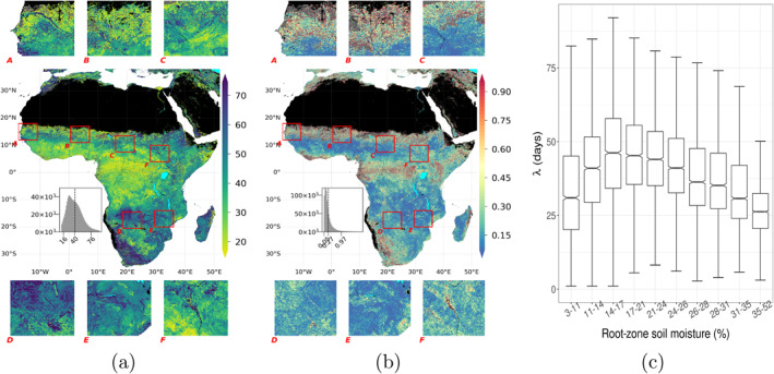
(a) e‐folding time of FVC time series during dry‐down (in days), λ, (b) variation of λ, and (c) distribution of λ within soil moisture. See Figure 2 for plotting details.

Besides the coherent continental‐scale spatial patterns, λ also has strong variations over meso‐scales. Stronger lateral moisture convergence positively affects the λ in arid regions, as seen in the Senegal (Box‐A, Figure 5a) and the Niger (partially in Box‐B, Figure 5a) rivers' riparian zones in the arid climate. However, lateral moisture convergence does not always affect λ positively, as seen in the riparian zones of the Upper Zambezi and the Okavango rivers and their tributaries. Shown in Box‐D in Figure 5a, λ is high around the Cuando river, the Okavango Delta and the Linyanti swamp, but low in the Barotse Floodplain (see Cronberg et al. [1995] and Zimba et al. [2018] for general information about the region). Such non‐trivial patterns suggest the role of complex interactions between the vegetation traits and local moisture conditions (Fan et al., 2019), which also affect λ.

4.3.1. λ and Ecosystem Water Use

We tested the last hypothesis of this study by analyzing the variations in λ conditioned against soil moisture, canopy height and tree cover, and grounded this to similar studies on ecosystem scale decay rates. λ can corroborate the rate of decrease of plant available water, ecosystem scale water use efficiency, and the propensity to senescence. Ecosystems differ widely in their water use strategies, from being water conservative—typically associated with strong down‐regulation of stomatal conductance with water deficiency—to aggressive exploitation of water resources (Laio et al., 2001). Herbaceous plants are typically aggressive water users and cease with the depletion of surface soil moisture. Woody plants risk cavitation and death under severe water stress, and such, trees in places with frequent dry periods benefit from a water saving strategy or senescence for prolonged periods. Konings and Gentine (2017) inferred ecosystem water‐use strategies globally based on diurnal variations of vegetation optical depth assuming that those reflect stomatal regulation to maintain leaf‐water potential. They found an increase in isohydricity, that is, the degree of stomatal regulation and subsequent water savings, with increase in vegetation height, consistent with the need of tall trees to prevent hydraulic failure during drought. Teuling et al. (2006) characterized decay rate in land evaporation (soil evaporation and transpiration) under water limitation using flux tower measurements and found that sites with stronger seasonality and larger woody coverage have slower decays. This association is supported by similar studies, for seasonality and canopy height (Boese et al., 2019), and for differences in the responses of trees and grasses (Martínez‐de la Torre et al., 2019). Slower decay of land evaporation of taller/woody canopy despite the faster decay of soil moisture with stronger aridity (McColl et al., 2017) suggests reduced transpiration or other plant adaptation mechanisms.

If the rate of FVC decay was also related to ecosystems' water use strategy in a similar manner, we would expect slower FVC decay (higher λ) with increasing canopy height. In regions with strong to intermediate aridity, we indeed find a tendency of increasing λ with canopy height except very tall canopy (Figure 6b), suggesting that λ incorporates ecosystem water use strategy traits as well as direct or indirect effects of soil moisture therein. However, as the climate gets wetter λ tends to decrease with canopy height. Possible explanations are that (a) changes in ecosystem scale drought coping strategies such as deep rooting (Singh et al., 2020), (b) water consumption, that is, transpiration, increases with canopy height resulting in a faster depletion of moisture storage (Koirala et al., 2017), or (c) increasing ecosystem water use efficiency with aridity.

Sensitivity of the nonlinear relationship between λ and climatological aridity to tree cover (see Figure 6b) shows that λ systematically increases with larger tree cover values in regions with high to intermediate aridity, where it peaks in regions with intermediate aridity and with 26%–43% of tree cover. This trend agrees with the reported interval for the transition from highly water‐stressed forest to savanna (Singh et al., 2020). However this pattern is inverted moving toward regions with weaker water‐stress, hence denser tree cover, which agrees with Singh et al. (2020) as moderately or lowly water‐stressed forests do not develop strong adaptation against water limitation, nor change canopy structure. The agreement among these two studies having different methodologies shows the value of the observation‐driven metric λ to gain ecohydrological insights and have a better understand in vegetation‐water dynamics.

5. Summary and Perspectives

Using retrievals of the SEVIRI sensor of the geostationary satellite MSG, we derived ecohydrological metrics for continental Africa entirely from the temporal dynamics of the daily Fraction of Vegetation Cover (FVC) time series from 2004 to 2019 at ca. 5 km (0.0417°) spatial resolution. Our metrics captures both continental scale gradients and covariations with climate as well as structured regional variations, for example, due to topographic factors. This provides an unprecedented opportunity to improve our understanding of ecohydrological processes across spatial scales over Africa.

We tested whether FVC_min or FVC_max are elevated in sandy soils due to the “inverse texture effect” and we found no evidence for this hypothesis, which, however could be also due to scale issues or uncertainty of the soil product. We further tested if access to secondary moisture sources such as groundwater generates “green islands” by increased FVC_min for topographic moisture indices. Also this hypothesis was not supported at continental scale, although riparian corridors, seasonal wetlands and floodplains are visually evident in FVC_min regionally. In contrast, and somewhat surprisingly, we found evidence for elevated FVC_max with increased topographic moisture conditions in dry regions. It suggests that in dry regions, the vegetation benefits from topographically induced secondary moisture input during the rainy season, while in the dry season water limitation is too severe for the vegetation to benefit from this secondary input. Our results imply that the patterns of FVC_max help diagnosing effects of secondary water resources in water limited regions. We analyzed to what extent the integral of FVC time series in decay period (I _dp ) reflects expected variations of the plant storage capacity or rooting depth. We found broad consistency between I _dp variations and aridity that are in agreement with theoretical considerations of rooting depth, and reasonable correlations with independent products of inferred plant water storage capacity. While the large uncertainty of independent evidence for variations of plant storage capacity precludes a more precise evaluation, our analysis suggests that I _dp is useful to diagnose variations in the buffering capacity of vegetation driven by moisture limitation. Finally, we analyzed whether the FVC decay rate during dry‐down (λ) follows patterns expected for soil moisture or decay time scale of terrestrial evaporation. Generally, the continental scale patterns against aridity and its sensitivity to canopy height and tree cover of λ agrees broadly with the plant adaptation strategies proposed in the literature. It seems λ indeed contains signatures of the complex ecohydrological interactions between moisture availability and vegetation. Clearly structured variations of λ at meso‐scales motivate in‐depth analyses of the metric to better understand ecohydrological interactions at finer scales, yet over a continental gradient.

Overall, given the the large amount of information stored in spatial variations of the metrics reflecting different driving mechanisms across spatial scales, the metrics have great potential to improve our understanding on vegetation dynamics on: (a) testing hypotheses on understanding relevance of local‐scale ecohydrological processes over large domains like continental Africa, (b) better understanding basic ecosystem properties like water usage in ecosystem scale and diagnosing their driving factors, and (c) extracting information and reducing uncertainty on concepts like plant water storage capacity.

Our ecohydrological metrics can help improving simulations of vegetation‐water cycle interactions by providing an observational basis for model evaluation and parameterizations. Since land surface models simulate vegetation cover fraction, the same ecohydrological metrics derived from simulated FVC can be computed using the code we provide. This has the advantage that multiple processes affecting FVC at different temporal scales—such as leaf shedding, adjustments in leaf area and canopy height, and differential responses of trees and grasses—are accounted for. A consistent and parallel assessment between observed and modeled variations of the ecohydrological metrics with relevant factors, such as those presented in this paper, can uncover model deficiencies and provide indications which processes or model parameters require attention. In a step further, these patterns of model data mismatch can be included in model calibration exercises to improve land surface models. As the spatialization of vegetation related parameters remains to be a major challenge (Fisher & Koven, 2020) our ecohydrological metrics can also facilitate exploring alternatives to the plant functional type paradigm. For example, one could test if a linear scaling of the spatial I _dp field to spatialize parameters controlling vegetation water storage capacity is sufficient, or better than plant functional type specific parameters (see e.g., Trautmann et al., 2021). Similarly, one could test if model parameters controlling drydown rates (see e.g., Raoult et al., 2021) can be better spatialized using our λ map than by using plant functional types. Our initial analyses points the importance of topographic effects against moisture limitation, emerging from lateral convergence and spatial heterogeneity that are mostly not represented in the models (Clark et al., 2015). This motivates for in‐depth analysis of the spatial variation of the metrics presented here to resolve and quantify importance of nontrivial components of water cycle against water limitation.

There remain multiple opportunities for further synergistic exploitation with retrievals of surface temperature from geostationary satellites which could provide complementary indicators on variations of moisture states inferred from an energy balance perspective. The suggested algorithms for deriving the metrics and the provision of the code facilitates parallel assessments and helps overcome the technical difficulties of dealing with large volumes of data and the particularities of vegetation cover retrievals from the geostationary satellites.

Appendix A. An Example Map of the Original FVC Data for a Single Day

Figure A1.

Figure A1.

The original FVC data product for a single day, taken from https://landsaf.ipma.pt/en/products/vegetation/fvc/.

Appendix B. Time Series of FVC in Example Grid Cells

In this subsection; we present 5 years time series of selected grid cells from each bin of mean annual soil moisture values given in the main manuscript to demonstrate the results of the algorithms in grid cell scale (Figures B1 and B2).

Figure B1.

FVC, soil moisture, and precipitation time series of sampled grid cells. Sampling is done to have one grid cell per each bin of soil moisture values given in the plots of the main manuscript. Points for both FVC and soil moisture are colored according to the state of vegetation activity as growing period is shown in light gray, decay period with dark gray while dry‐down during the decay period is shown in black. Fitted curve to estimate λ is shown with red lines while 31‐day smoothed FVC values are shown in orange lines at the upper panel, while daily precipitation values are shown with blue bars at the lower panel. Note that daily aggregated precipitation data is obtained from Tropical Rainfall Measuring Mission (TRMM) (2011).

Figure B2.

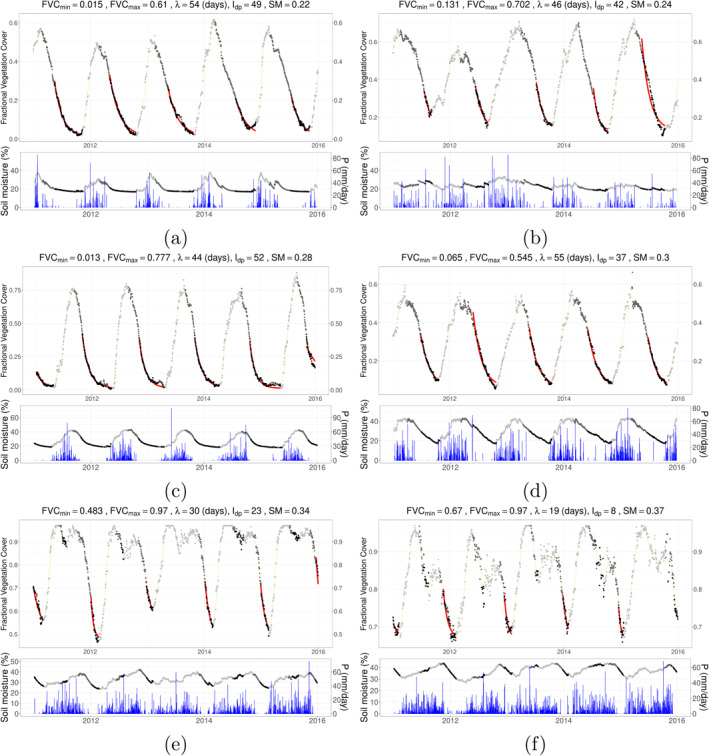
Continuation of Figure B1 with samples having larger mean annual soil moisture.

Appendix C. Density Plots of the Ecohydrological Metrics

Figure C1.

Figure C1.

Density plots of the ecohydrological metrics presented in this study.

Appendix D. Temporal Correlation Between FVC and Soil Moisture

Figure D1.

Figure D1.

Pixelwise Spearman's correlation of FVC and GLEAM root‐zone soil moisture in time for (a) entire time series and (b) time series marked as decay period using FVC.

Appendix E. Map of Climatological Aridity and Google Earth View of Insets

Figure E1 shows the continental map of mean annual root‐zone soil moisture (%) from GLEAM and the Google Earth views of the insets. Note that soil moisture values are binned to have equal number of observations in each class. Box‐A: the Gambia and large portion of the Senegal rivers; Box‐B: a small area of the Niger river mostly showing the transition from the Sahara desert to Sahel; Box‐C: more on the transition from Sahel to tropical regions; Box‐D: located in one of the most complex regions of Africa in terms of topography and lateral flow of water with lower sections of the Okavango and the Cuando rivers and upper section of the Zambezi river, together with multiple seasonally flooding areas like the Okavango delta, the Barotse Floodplain, and the Linyanti swamp. These seasonal wetlands are vital for the ecosystem and also provides great support against water limitation and heat for not only plants but also animals; Box‐E: Lower Zambezi Basin together with the drainage of Lake Malawi to Zambezi. It also covers the Inyanga mountains located between Mozambique and Zimbabwe where a climatic shift happens over the mountain range. Last but not least, Box‐F: largely covered by tropical savanna, is divided by the White Nile from South to North, covers the Sudd swamp.

Figure E1.

Map of mean annual root‐zone soil moisture (%) in the center and satellite view of the insets. Map and image data of the insets: Google Earth ©2020 TerraMetrics.

Appendix F. Heatmaps of Raw Values of Asymptote‐Related Metrics

Figure F1.

Figure F1.

Covariation of asymptote‐related metrics and root‐zone soil moisture with sand percentage, HAND, and TWI. Note that binning of the continuous variables in x‐ and y‐axes are done automatically to equalize frequency of observations among the bins of a given variable.

Appendix G. Summary of Seasonal Dynamics of FVC, FVC_range

Figure G1.

Figure G1.

Variations in FVC_range (as FVC_max − FVC_min) (a) in space (b) with climatological aridity (c) similar to Figure 3a but for FVC_range (d) similar to Figure F1a but for FVC_range.

Appendix H. Map of I _dp Normalized by Event Duration

In order to see the effect of event duration to I _dp , we normalized the I _dp values with the duration of the specific event I _dp is estimated. Even though spatial patterns remained largely the same after normalization, they became more pronounced in the East Sudanian Savanna and Miombo woodlands in the Southern Africa. Spatial distribution of the normalized I _dp is mapped, together with its covariation with soil moisture and the original I _dp is shown in Figure H1. Note that duration of the event necessary to make the normalization is available in the corresponding netCDF file of the metrics (see Section 6).

Figure H1.

Integral of FVC time series in the decay period normalized by event duration (a) Spatial variation, (b) variation against within mean annual soil moisture (see Figure 2c for plotting details). (c) Density plot against I _dp .

Appendix I. Map of Number of Convergences of Algorithm 2

Figure I1.

Figure I1.

Number of decay periods in which the Algorithm 2 successfully converged.

Appendix J. Maps of Accessible Water Storage Capacity Data Sets

Figure J1.

Figure J1.

Maps of accessible water storage capacity and Rooting Depth (RD) data sets used in this study. (a) Integral of FVC during decay period, I _dp , (b) Root Zone Storage Capacity (RZS _CRU2) using CRU as precipitation forcing data with 2 years of drought return period from Wang‐Erlandsson et al. (2016), (c) Accessible Water Storage Capacity from S. Tian et al. (2019) (d) Effective Rooting Depth from Yang et al. (2016), (e) RD from Fan et al. (2017). All products are aggregated to 0.5° and cropped for the study domain.

Küçük, Ç. , Koirala, S. , Carvalhais, N. , Miralles, D. G. , Reichstein, M. , & Jung, M. (2022). Characterizing the response of vegetation cover to water limitation in Africa using geostationary satellites. Journal of Advances in Modeling Earth Systems, 14, e2021MS002730. 10.1029/2021MS002730

Data Availability Statement

All ecohydrological metrics presented in this study are available in standardized netCDF data format in https://doi.org/10.6084/m9.figshare.14987211.v1, together with their quality diagnostics. The R scripts developed for the implementation of the methodology are available for research uses. They can be accessed through https://github.com/caglarkucuk/EcohydroMetrics_Africa.git. All the data used in this study are available in the cited literature (see Section 2), except the AWSC data from S. Tian et al. (2019) which was obtained from the corresponding author.

References

- Adole, T. , Dash, J. , & Atkinson, P. M. (2016). A systematic review of vegetation phenology in Africa. Ecological Informatics, 34, 117–128. 10.1016/j.ecoinf.2016.05.004 [DOI] [Google Scholar]
- Adole, T. , Dash, J. , Rodriguez‐Galiano, V. , & Atkinson, P. M. (2019). Photoperiod controls vegetation phenology across Africa. Communications Biology, 2(1). 10.1038/s42003-019-0636-7 [DOI] [PMC free article] [PubMed] [Google Scholar]
- Akasheh, O. Z. , Neale, C. M. , & Jayanthi, H. (2008). Detailed mapping of riparian vegetation in the middle Rio Grande River using high resolution multi‐spectral airborne remote sensing. Journal of Arid Environments, 72(9), 1734–1744. 10.1016/j.jaridenv.2008.03.014 [DOI] [Google Scholar]
- Amatulli, G. , McInerney, D. , Sethi, T. , Strobl, P. , & Domisch, S. (2020). Geomorpho90m, empirical evaluation and accuracy assessment of global high‐resolution geomorphometric layers. Scientific Data, 7(1), 1–18. 10.1038/s41597-020-0479-6 [DOI] [PMC free article] [PubMed] [Google Scholar]
- Anderegg, W. R. , Konings, A. G. , Trugman, A. T. , Yu, K. , Bowling, D. R. , Gabbitas, R. , et al. (2018). Hydraulic diversity of forests regulates ecosystem resilience during drought. Nature, 561(7724), 538–541. 10.1038/s41586-018-0539-7 [DOI] [PubMed] [Google Scholar]
- Barron, O. V. , Emelyanova, I. , Van Niel, T. G. , Pollock, D. , & Hodgson, G. (2014). Mapping groundwater‐dependent ecosystems using remote sensing measures of vegetation and moisture dynamics. Hydrological Processes, 28(2), 372–385. 10.1002/hyp.9609 [DOI] [Google Scholar]
- Beck, P. S. A. , Atzberger, C. , Høgda, K. A. , Johansen, B. , & Skidmore, A. K. (2006). Improved monitoring of vegetation dynamics at very high latitudes: A new method using MODIS NDVI. Remote Sensing of Environment, 100(3), 321–334. 10.1016/j.rse.2005.10.021 [DOI] [Google Scholar]
- Boese, S. , Jung, M. , Carvalhais, N. , Teuling, A. J. , & Reichstein, M. (2019). Carbon‐water flux coupling under progressive drought. Biogeosciences, 16(13), 2557–2572. 10.5194/bg-16-2557-2019 [DOI] [Google Scholar]
- Caylor, K. K. , Manfreda, S. , & Rodriguez‐Iturbe, I. (2005). On the coupled geomorphological and ecohydrological organization of river basins. Advances in Water Resources, 28(1), 69–86. 10.1016/j.advwatres.2004.08.013 [DOI] [Google Scholar]
- Caylor, K. K. , Scanlon, T. M. , & Rodríguez‐Iturbe, I. (2009). Ecohydrological optimization of pattern and processes in water‐limited ecosystems: A trade‐off‐based hypothesis. Water Resources Research, 45(8), 1–15. 10.1029/2008WR007230 [DOI] [Google Scholar]
- Clark, M. P. , Fan, Y. , Lawrence, D. M. , Adam, J. C. , Bolster, D. , Gochis, D. J. , et al. (2015). Improving the representation of hydrologic processes in Earth System Models. Water Resources Research, 51(8), 5929–5956. 10.1002/2015WR017096 [DOI] [Google Scholar]
- Cronberg, G. , Gieske, A. , Martins, E. , Prince Nengu, J. , & Stenström, I.‐M. (1995). Hydrobiological studies of the Okavango Delta and Kwando/Linyati/Chobe River, Botswana I surface water quality analysis. Botswana Notes and Records (Vol. 27). Retrieved from http://www.jstor.org/stable/40980045 [Google Scholar]
- Dimiceli, C. , Carroll, M. , Sohlberg, R. , Kim, D. H. , Kelly, M. , & Townshend, J. R. G. (2015). MOD44B MODIS/Terra vegetation continuous fields yearly L3 global 250m SIN grid V006. NASA EOSDIS Land Processes DAAC. 10.5067/MODIS/MOD44B.006 [DOI] [Google Scholar]
- D’Odorico, P. , Porporato, A. , & Runyan, C. W. (2019). Dryland ecohydrology. Springer International Publishing. 10.1007/978-3-030-23269-6 [DOI] [Google Scholar]
- Eamus, D. , Zolfaghar, S. , Villalobos‐Vega, R. , Cleverly, J. , & Huete, A. (2015). Groundwater‐dependent ecosystems: Recent insights from satellite and field‐based studies. Hydrology and Earth System Sciences, 19(10), 4229–4256. 10.5194/hess-19-4229-2015 [DOI] [Google Scholar]
- Elzhov, T. V. , Mullen, K. M. , Spiess, A.‐N. , & Bolker, B. (2016). minpack.lm: R interface to the Levenberg‐Marquardt nonlinear least‐squares algorithm found in MINPACK [Computer software manual]. Plus Support for Bounds. Retrieved from https://cran.r-project.org/package=minpack.lm
- Epstein, H. E. , Lauenroth, W. K. , & Burke, I. C. (1997). Effects of temperature and soil texture on ANPP in the U.S. Great Plains. Ecology, 78(8), 2628–2631. 10.1890/0012-9658(1997)078[2628:eotast]2.0.co;2 [DOI] [Google Scholar]
- Everitt, J. H. , & Deloach, C. J. (1990). Remote sensing of Chinese tamarisk (Tamarix chinensis) and associated vegetation. Weed Science, 38(3), 273–278. 10.1017/S0043174500056526 [DOI] [Google Scholar]
- Everitt, J. H. , Judd, F. W. , Escobar, D. E. , Alaniz, M. A. , Davis, M. R. , & Macwhorter, W. (1996). Using remote sensing and spatial information technologies to map sabal palm in the lower Rio Grande Valley of Texas. Southwestern Naturalist, 41(3), 218–226. [Google Scholar]
- Fan, Y. , Clark, M. , Lawrence, D. M. , Swenson, S. , Band, L. E. , Brantley, S. L. , et al. (2019). Hillslope hydrology in global change research and Earth system modeling. Water Resources Research, 55, 1737–1772. 10.1029/2018WR023903 [DOI] [Google Scholar]
- Fan, Y. , Miguez‐Macho, G. , Jobbágy, E. G. , Jackson, R. B. , & Otero‐Casal, C. (2017). Hydrologic regulation of plant rooting depth. Proceedings of the National Academy of Sciences, 114(40), 10572–10577. 10.1073/pnas.1712381114 [DOI] [PMC free article] [PubMed] [Google Scholar]
- Fernandez‐Illescas, C. P. , Porporato, A. , Laio, F. , & Rodríguez‐Iturbe, I. (2001). The ecohydrological role of soil texture in a water‐limited ecosystem. Water Resources Research, 37(12), 2863–2872. 10.1029/2000WR000121 [DOI] [Google Scholar]
- Fisher, R. A. , & Koven, C. D. (2020). Perspectives on the future of land surface models and the challenges of representing complex terrestrial systems. Journal of Advances in Modeling Earth Systems, 12. 10.1029/2018ms001453 [DOI] [Google Scholar]
- García‐Haro, F. J. , Camacho, F. , Martínez, B. , Campos‐Taberner, M. , Fuster, B. , Sánchez‐Zapero, J. , & Gilabert, M. A. (2019). Climate data records of vegetation variables from geostationary SEVIRI/MSG data: Products, algorithms and applications. Remote Sensing, 11(18), 2103. 10.3390/rs11182103 [DOI] [Google Scholar]
- GDAL/OGR contributors . (2020). GDAL/OGR geospatial data abstraction software library [Computer software manual]. Open Source Geospatial Foundation. Retrieved from https://gdal.org
- Gentine, P. , D’Odorico, P. , Lintner, B. R. , Sivandran, G. , & Salvucci, G. (2012). Interdependence of climate, soil, and vegetation as constrained by the Budyko curve. Geophysical Research Letters, 39(19). 10.1029/2012GL053492 [DOI] [Google Scholar]
- Gond, V. , Fayolle, A. , Pennec, A. , Cornu, G. , Mayaux, P. , Camberlin, P. , et al. (2013). Vegetation structure and greenness in Central Africa from MODIS multi‐temporal data. Philosophical Transactions of the Royal Society B: Biological Sciences, 368(1625), 20120309. 10.1098/rstb.2012.0309 [DOI] [PMC free article] [PubMed] [Google Scholar]
- Guan, K. , Medvigy, D. , Wood, E. F. , Caylor, K. K. , Li, S. , & Jeong, S. J. (2014). Deriving vegetation phenological time and trajectory information over Africa using SEVIRI daily LAI. IEEE Transactions on Geoscience and Remote Sensing, 52(2), 1113–1130. 10.1109/TGRS.2013.2247611 [DOI] [Google Scholar]
- Guan, K. , Pan, M. , Li, H. , Wolf, A. , Wu, J. , Medvigy, D. , et al. (2015). Photosynthetic seasonality of global tropical forests constrained by hydroclimate. Nature Geoscience, 8(4), 284–289. 10.1038/ngeo2382 [DOI] [Google Scholar]
- Guan, K. , Wolf, A. , Medvigy, D. , Caylor, K. K. , Pan, M. , & Wood, E. F. (2013). Seasonal coupling of canopy structure and function in African tropical forests and its environmental controls. Ecosphere, 4(3), 1–21. 10.1890/ES12-00232.1 [DOI] [Google Scholar]
- Guan, K. , Wood, E. F. , Medvigy, D. , Kimball, J. , Pan, M. , Caylor, K. K. , et al. (2014). Terrestrial hydrological controls on land surface phenology of African savannas and woodlands. Journal of Geophysical Research: Biogeosciences, 119(8), 1652–1669. 10.1002/2013JG002572 [DOI] [Google Scholar]
- Guswa, A. J. (2008). The influence of climate on root depth: A carbon cost‐benefit analysis. Water Resources Research, 44(2), 1–11. 10.1029/2007WR006384 [DOI] [Google Scholar]
- Guswa, A. J. (2010). Effect of plant uptake strategy on the water‐optimal root depth. Water Resources Research, 46(9), 1–5. 10.1029/2010WR009122 [DOI] [Google Scholar]
- Harris, I. , Jones, P. D. , Osborn, T. J. , & Lister, D. H. (2014). Updated high‐resolution grids of monthly climatic observations—The CRU TS3.10 Dataset. International Journal of Climatology, 34(3), 623–642. 10.1002/joc.3711 [DOI] [Google Scholar]
- Hengl, T. , Mendes de Jesus, J. , Heuvelink, G. B. , Gonzalez, M. R. , Kilibarda, M. , Blagotić, A. , et al. (2017). SoilGrids250m: Global gridded soil information based on machine learning. PLoS One, 12(2), 1–40. 10.1371/journal.pone.0169748 [DOI] [PMC free article] [PubMed] [Google Scholar]
- Herrmann, S. M. , & Mohr, K. I. (2011). A continental‐scale classification of rainfall seasonality regimes in Africa based on gridded precipitation and land surface temperature products. Journal of Applied Meteorology and Climatology, 50(12), 2504–2513. 10.1175/JAMC-D-11-024.1 [DOI] [Google Scholar]
- Howard, J. , & Merrifield, M. (2010). Mapping groundwater dependent ecosystems in California. PLoS One, 5(6), e11249. 10.1371/journal.pone.0011249 [DOI] [PMC free article] [PubMed] [Google Scholar]
- Jacobson, P. J. , & Jacobson, K. M. (2013). Hydrologic controls of physical and ecological processes in Namib Desert ephemeral rivers: Implications for conservation and management. Journal of Arid Environments, 93, 80–93. 10.1016/j.jaridenv.2012.01.010 [DOI] [Google Scholar]
- Jin, X. M. , Schaepman, M. E. , Clevers, J. G. , Su, Z. B. , & Hu, G. C. (2011). Groundwater depth and vegetation in the Ejina area, China. Arid Land Research and Management, 25(2), 194–199. 10.1080/15324982.2011.554953 [DOI] [Google Scholar]
- Kleidon, A. , & Heimann, M. (1998). A method of determining rooting depth from a terrestrial biosphere model and its impacts on the global water and carbon cycle. Global Change Biology, 4(3), 275–286. 10.1046/j.1365-2486.1998.00152.x [DOI] [Google Scholar]
- Koirala, S. , Jung, M. , Reichstein, M. , de Graaf, I. E. , Camps‐Valls, G. , Ichii, K. , et al. (2017). Global distribution of groundwater‐vegetation spatial covariation. Geophysical Research Letters, 44(9), 4134–4142. 10.1002/2017GL072885 [DOI] [Google Scholar]
- Konings, A. G. , & Gentine, P. (2017). Global variations in ecosystem‐scale isohydricity. Global Change Biology, 23(2), 891–905. 10.1111/gcb.13389 [DOI] [PubMed] [Google Scholar]
- Kuppel, S. , Fan, Y. , & Jobbágy, E. G. (2017). Seasonal hydrologic buffer on continents: Patterns, drivers and ecological benefits. Advances in Water Resources, 102, 178–187. 10.1016/j.advwatres.2017.01.004 [DOI] [Google Scholar]
- Laio, F. , D’Odorico, P. , & Ridolfi, L. (2006). An analytical model to relate the vertical root distribution to climate and soil properties. Geophysical Research Letters, 33(18). 10.1029/2006GL027331 [DOI] [Google Scholar]
- Laio, F. , Porporato, A. , Fernandez‐Illescas, C. P. , & Rodríguez‐Iturbe, I. (2001). Plants in water‐controlled ecosystems: Active role in hydrologic processes and response to water stress IV. Discussion of real cases. Advances in Water Resources, 24(7), 745–762. 10.1016/S0309-1708(01)00007-0 [DOI] [Google Scholar]
- Liu, Y. , Kumar, M. , Katul, G. G. , & Porporato, A. (2019). Reduced resilience as an early warning signal of forest mortality. Nature Climate Change, 9(11), 880–885. 10.1038/s41558-019-0583-9 [DOI] [Google Scholar]
- Looney, C. E. , Sullivan, B. W. , Kolb, T. E. , Kane, J. M. , & Hart, S. C. (2012). Pinyon pine (Pinus edulis) mortality and response to water addition across a three million year substrate age gradient in northern Arizona, USA. Plant and Soil, 357(1), 89–102. 10.1007/s11104-012-1150-6 [DOI] [Google Scholar]
- LSA‐SAF . (2016). Algorithm theoretical basis document for vegetation parameters (VEGA) (Technical Report, Version 2.0). Retrieved from https://landsaf.ipma.pt/en/products/vegetation/fvc/ [Google Scholar]
- Ludwig, J. A. , Wilcox, B. P. , Breshears, D. D. , Tongway, D. J. , & Imeson, A. C. (2005). Vegetation patches and runoff‐erosion as interacting ecohydrological processes in semiarid landscapes. Ecology, 86(2), 288–297. 10.1890/03-0569 [DOI] [Google Scholar]
- Lv, J. , Wang, X. S. , Zhou, Y. , Qian, K. , Wan, L. , Eamus, D. , & Tao, Z. (2013). Groundwater‐dependent distribution of vegetation in Hailiutu River catchment, a semi‐arid region in China. Ecohydrology, 6(1), 142–149. 10.1002/eco.1254 [DOI] [Google Scholar]
- MacBean, N. , Scott, R. L. , Biederman, J. A. , Peylin, P. , Kolb, T. , Litvak, M. E. , et al. (2021). Dynamic global vegetation models underestimate net CO2 flux mean and inter‐annual variability in dryland ecosystems. Environmental Research Letters, 16(9), 094023. 10.1088/1748-9326/ac1a38 [DOI] [Google Scholar]
- Mansell, M. G. , & Hussey, S. W. (2005). An investigation of flows and losses within the alluvial sands of ephemeral rivers in Zimbabwe. Journal of Hydrology, 314(1–4), 192–203. 10.1016/j.jhydrol.2005.03.015 [DOI] [Google Scholar]
- Martens, B. , Miralles, D. G. , Lievens, H. , Van Der Schalie, R. , De Jeu, R. A. , Fernández‐Prieto, D. , et al. (2017). GLEAM v3: Satellite‐based land evaporation and root‐zone soil moisture. Geoscientific Model Development, 10(5), 1903–1925. 10.5194/gmd-10-1903-2017 [DOI] [Google Scholar]
- Martens, C. , Hickler, T. , Davis‐Reddy, C. , Engelbrecht, F. , Higgins, S. I. , von Maltitz, G. P. , et al. (2021). Large uncertainties in future biome changes in Africa call for flexible climate adaptation strategies. Global Change Biology, 27(2), 340–358. 10.1111/gcb.15390 [DOI] [PubMed] [Google Scholar]
- Martínez‐de la Torre, A. , Blyth, E. M. , & Robinson, E. L. (2019). Evaluation of drydown processes in global land surface and hydrological models using flux tower evapotranspiration. Water, 11, 356. 10.3390/w11020356 [DOI] [Google Scholar]
- McCarthy, T. S. (2006). Groundwater in the wetlands of the Okavango Delta, Botswana, and its contribution to the structure and function of the ecosystem. Journal of Hydrology, 320(3–4), 264–282. 10.1016/j.jhydrol.2005.07.045 [DOI] [Google Scholar]
- McColl, K. A. , Wang, W. , Peng, B. , Akbar, R. , Short Gianotti, D. J. , Lu, H. , et al. (2017). Global characterization of surface soil moisture drydowns. Geophysical Research Letters, 44(8), 3682–3690. 10.1002/2017GL072819 [DOI] [Google Scholar]
- Merbold, L. , Ardö, J. , Arneth, A. , Scholes, R. J. , Nouvellon, Y. , De Grandcourt, A. , et al. (2009). Precipitation as driver of carbon fluxes in 11 African ecosystems. Biogeosciences, 6(6), 1027–1041. 10.5194/bg-6-1027-2009 [DOI] [Google Scholar]
- Miralles, D. G. , Holmes, T. R. , De Jeu, R. A. , Gash, J. H. , Meesters, A. G. , & Dolman, A. J. (2011). Global land‐surface evaporation estimated from satellite‐based observations. Hydrology and Earth System Sciences, 15(2), 453–469. 10.5194/hess-15-453-2011 [DOI] [Google Scholar]
- Moré, J. J. (1978). The Levenberg‐Marquardt algorithm: Implementation and theory. In Watson G. A. (Ed.), Lecture notes in mathematics (pp. 105–116). Springer‐Verlag. 10.1007/bfb0067700 [DOI] [Google Scholar]
- Müller, C. , Waha, K. , Bondeau, A. , & Heinke, J. (2014). Hotspots of climate change impacts in sub‐Saharan Africa and implications for adaptation and development. Global Change Biology, 20(8), 2505–2517. 10.1111/gcb.12586 [DOI] [PubMed] [Google Scholar]
- Münch, Z. , & Conrad, J. (2007). Remote sensing and GIS based determination of groundwater dependent ecosystems in the Western Cape, South Africa. Hydrogeology Journal, 15(1), 19–28. 10.1007/s10040-006-0125-1 [DOI] [Google Scholar]
- Nash, E. , & Sutcliffe, V. (1970). River flow forecasting through conceptual models part I—A discussion of principles. Journal of Hydrology, 10, 282–290. 10.1016/0022-1694(70)90255-6 [DOI] [Google Scholar]
- Neale, C. M. (1997). Classification and mapping of riparian systems using airborne multispectral videography. Restoration Ecology, 5, 103–112. 10.1111/j.1526-100X.1997.00103.x [DOI] [Google Scholar]
- Nelson, J. A. , Pérez‐Priego, O. , Zhou, S. , Poyatos, R. , Zhang, Y. , Blanken, P. D. , et al. (2020). Ecosystem transpiration and evaporation: Insights from three water flux partitioning methods across FLUXNET sites. Global Change Biology, 26(12), 6916–6930. 10.1111/gcb.15314 [DOI] [PubMed] [Google Scholar]
- Newman, B. D. , Wilcox, B. P. , Archer, S. R. , Breshears, D. D. , Dahm, C. N. , Duffy, C. J. , et al. (2006). Ecohydrology of water‐limited environments: A scientific vision. Water Resources Research, 42(6), 1–15. 10.1029/2005WR004141 [DOI] [Google Scholar]
- Nobre, A. D. , Cuartas, L. A. , Hodnett, M. , Rennó, C. D. , Rodrigues, G. , Silveira, A. , et al. (2011). Height Above the Nearest Drainage—A hydrologically relevant new terrain model. Journal of Hydrology, 404(1–2), 13–29. 10.1016/j.jhydrol.2011.03.051 [DOI] [Google Scholar]
- Noy‐Meir, I. (1973). Desert ecosystems: Environment and producers. Annual Review of Ecology and Systematics, 4(1), 25–51. 10.1146/annurev.es.04.110173.000325 [DOI] [Google Scholar]
- Ouédraogo, D. Y. , Hardy, O. J. , Doucet, J. L. , Janssens, S. B. , Wieringa, J. J. , Stoffelen, P. , et al. (2020). Latitudinal shift in the timing of flowering of tree species across tropical Africa: Insights from field observations and herbarium collections. Journal of Tropical Ecology, 36, 159–173. 10.1017/S0266467420000103 [DOI] [Google Scholar]
- Palmer, P. I. , Feng, L. , Baker, D. , Chevallier, F. , Bösch, H. , & Somkuti, P. (2019). Net carbon emissions from African biosphere dominate pan‐tropical atmospheric CO2 signal. Nature Communications, 10(1), 1–9. 10.1038/s41467-019-11097-w [DOI] [PMC free article] [PubMed] [Google Scholar]
- Paschalis, A. , Fatichi, S. , Zscheischler, J. , Ciais, P. , Bahn, M. , Boysen, L. , et al. (2020). Rainfall manipulation experiments as simulated by terrestrial biosphere models: Where do we stand? Global Change Biology, 26(6), 3336–3355. 10.1111/gcb.15024 [DOI] [PubMed] [Google Scholar]
- Peñuelas, J. , Filella, I. , Zhang, X. , Llorens, L. , Ogaya, R. , Lloret, F. , et al. (2004). Complex spatiotemporal phenological shifts as a response to rainfall changes. New Phytologist, 161(3), 837–846. 10.1111/j.1469-8137.2004.01003.x [DOI] [PubMed] [Google Scholar]
- Porporato, A. , Laio, F. , Ridolfi, L. , & Rodríguez‐Iturbe, I. (2001). Plants in water‐controlled ecosystems: Active role in hydrologic processes and response to water stress: III. Vegetation water stress. Advances in Water Resources, 24(7), 725–744. 10.1016/S0309-1708(01)00006-9 [DOI] [Google Scholar]
- Raduła, M. W. , Szymura, T. H. , & Szymura, M. (2018). Topographic wetness index explains soil moisture better than bioindication with Ellenberg’s indicator values. Ecological Indicators, 85, 172–179. 10.1016/j.ecolind.2017.10.011 [DOI] [Google Scholar]
- Raoult, N. , Ottlé, C. , Peylin, P. , Bastrikov, V. , & Maugis, P. (2021). Evaluating and optimizing surface soil moisture drydowns in the ORCHIDEE land surface model at in situ locations. Journal of Hydrometeorology, 22(4), 1025–1043. 10.1175/jhm-d-20-0115.1 [DOI] [Google Scholar]
- Rodríguez‐Iturbe, I. , D’Odorico, P. , Porporato, A. , & Ridolfi, L. (1999). On the spatial and temporal links between vegetation, climate, and soil moisture. Water Resources Research, 35(12), 3709–3722. 10.1029/1999WR900255 [DOI] [Google Scholar]
- Rousseeuw, P. J. , & Croux, C. (1993). Alternatives to the median absolute deviation. Journal of the American Statistical Association, 88(424), 1273–1283. 10.1080/01621459.1993.10476408 [DOI] [Google Scholar]
- Sala, O. E. , Parton, W. J. , Joyce, L. A. , & Lauenroth, W. K. (1988). Primary production of the central grassland region of the United States. Ecology, 69(1), 40–45. 10.2307/1943158 [DOI] [Google Scholar]
- Sankaran, M. , Hanan, N. P. , Scholes, R. J. , Ratnam, J. , Augustine, D. J. , Cade, B. S. , et al. (2005). Determinants of woody cover in African savannas. Nature, 438(7069), 846–849. 10.1038/nature04070 [DOI] [PubMed] [Google Scholar]
- Sankaran, M. , Ratnam, J. , & Hanan, N. (2008). Woody cover in African savannas: The role of resources, fire and herbivory. Global Ecology and Biogeography, 17(2), 236–245. 10.1111/j.1466-8238.2007.00360.x [DOI] [Google Scholar]
- Scanlon, T. M. , Caylor, K. K. , Manfreda, S. , Levin, S. A. , & Rodríguez‐Iturbe, I. (2005). Dynamic response of grass cover to rainfall variability: Implications for the function and persistence of savanna ecosystems. Advances in Water Resources, 28(3), 291–302. 10.1016/j.advwatres.2004.10.014 [DOI] [Google Scholar]
- Schenk, H. J. (2008). The shallowest possible water extraction profile: A null model for global root distributions. Vadose Zone Journal, 7(3), 1119–1124. 10.2136/vzj2007.0119 [DOI] [Google Scholar]
- Schenk, H. J. , & Jackson, R. B. (2002). Rooting depths, lateral root spreads and belowground aboveground allometries of plants in water limited ecosystems. Journal of Ecology, 90, 480–494. 10.1046/j.1365-2745.2002.00682.x [DOI] [Google Scholar]
- Schmiedel, U. , Jacke, V. , Hachfeld, B. , & Oldeland, J. (2021). Response of Kalahari vegetation to seasonal climate and herbivory: Results of 15 years of vegetation monitoring. Journal of Vegetation Science, 32(1), 1–13. 10.1111/jvs.12927 [DOI] [Google Scholar]
- Simard, M. , Pinto, N. , Fisher, J. B. , & Baccini, A. (2011). Mapping forest canopy height globally with spaceborne lidar. Journal of Geophysical Research, 116(4), 1–12. 10.1029/2011JG001708 [DOI] [Google Scholar]
- Singh, C. , Wang‐Erlandsson, L. , Fetzer, I. , Rockström, J. , & Van Der Ent, R. (2020). Rootzone storage capacity reveals drought coping strategies along rainforest‐savanna transitions. Environmental Research Letters, 15(12), 124021. 10.1088/1748-9326/abc377 [DOI] [Google Scholar]
- Tao, S. , Guo, Q. , Li, C. , Wang, Z. , & Fang, J. (2016). Global patterns and determinants of forest canopy height. Ecology, 97(12), 3265–3270. 10.1002/ecy.1580 [DOI] [PubMed] [Google Scholar]
- Taylor, R. G. , Todd, M. C. , Kongola, L. , Maurice, L. , Nahozya, E. , Sanga, H. , & Macdonald, A. M. (2013). Evidence of the dependence of groundwater resources on extreme rainfall in East Africa. Nature Climate Change, 3(4), 374–378. 10.1038/nclimate1731 [DOI] [Google Scholar]
- Teuling, A. J. , Seneviratne, S. I. , Williams, C. , & Troch, P. A. (2006). Observed timescales of evapotranspiration response to soil moisture. Geophysical Research Letters, 33(23). 10.1029/2006GL028178 [DOI] [Google Scholar]
- Tian, F. , Wigneron, J. P. , Ciais, P. , Chave, J. , Ogée, J. , Peñuelas, J. , et al. (2018). Coupling of ecosystem‐scale plant water storage and leaf phenology observed by satellite. Nature Ecology and Evolution, 2(9), 1428–1435. 10.1038/s41559-018-0630-3 [DOI] [PubMed] [Google Scholar]
- Tian, S. , Van Dijk, A. I. , Tregoning, P. , & Renzullo, L. J. (2019). Forecasting dryland vegetation condition months in advance through satellite data assimilation. Nature Communications, 10(1), 1–7. 10.1038/s41467-019-08403-x [DOI] [PMC free article] [PubMed] [Google Scholar]
- Tootchi, A. , Jost, A. , & Ducharne, A. (2019). Multi‐source global wetland maps combining surface water imagery and groundwater constraints. Earth System Science Data, 11(1), 189–220. 10.5194/essd-11-189-2019 [DOI] [Google Scholar]
- Tooth, S. (2000). Process, form and change in dryland rivers: A review of recent research. Earth Science Reviews, 51(1–4), 67–107. 10.1016/S0012-8252(00)00014-3 [DOI] [Google Scholar]
- Trautmann, T. , Koirala, S. , Carvalhais, N. , Güntner, A. , & Jung, M. (2021). The importance of vegetation to understand terrestrial water storage variations. Hydrology and Earth System Sciences Discussions, 1–31. 10.5194/hess-2021-394 [DOI] [Google Scholar]
- Trigo, I. F. , Dacamara, C. C. , Viterbo, P. , Roujean, J. L. , Olesen, F. , Barroso, C. , et al. (2011). The satellite application facility for land surface analysis. International Journal of Remote Sensing, 32(10), 2725–2744. 10.1080/01431161003743199 [DOI] [Google Scholar]
- Tropical Rainfall Measuring Mission (TRMM) . (2011). TRMM (TMPA) rainfall estimate L3 V7. Goddard Earth Sciences Data and Information Services Center (GES DISC). 10.5067/TRMM/TMPA/3H/7 [DOI] [Google Scholar]
- Ukkola, A. M. , De Kauwe, M. G. , Roderick, M. L. , Burrell, A. , Lehmann, P. , & Pitman, A. J. (2021). Annual precipitation explains variability in dryland vegetation greenness globally but not locally. Global Change Biology, 27(18), 4367–4380. 10.1111/gcb.15729 [DOI] [PubMed] [Google Scholar]
- Valentini, R. , Arneth, A. , Bombelli, A. , Castaldi, S. , Cazzolla Gatti, R. , Chevallier, F. , et al. (2014). A full greenhouse gases budget of Africa: Synthesis, uncertainties, and vulnerabilities. Biogeosciences, 11(2), 381–407. 10.5194/bg-11-381-2014 [DOI] [Google Scholar]
- van Dijk, A. I. , Peña‐Arancibia, J. L. , Wood, E. F. , Sheffield, J. , & Beck, H. E. (2013). Global analysis of seasonal streamflow predictability using an ensemble prediction system and observations from 6192 small catchments worldwide. Water Resources Research, 49(5), 2729–2746. 10.1002/wrcr.20251 [DOI] [Google Scholar]
- van Wijk, M. T. (2011). Understanding plant rooting patterns in semi‐arid systems: An integrated model analysis of climate, soil type and plant biomass. Global Ecology and Biogeography, 20(2), 331–342. 10.1111/j.1466-8238.2010.00601.x [DOI] [Google Scholar]
- Wang, J. , Song, C. , Reager, J. T. , Yao, F. , Famiglietti, J. S. , Sheng, Y. , et al. (2018). Recent global decline in endorheic basin water storages. Nature Geoscience, 11(12), 926–932. 10.1038/s41561-018-0265-7 [DOI] [PMC free article] [PubMed] [Google Scholar]
- Wang‐Erlandsson, L. , Bastiaanssen, W. G. , Gao, H. , Jägermeyr, J. , Senay, G. B. , Van Dijk, A. I. , et al. (2016). Global root zone storage capacity from satellite‐based evaporation. Hydrology and Earth System Sciences, 20(4), 1459–1481. 10.5194/hess-20-1459-2016 [DOI] [Google Scholar]
- Weber, U. , Jung, M. , Reichstein, M. , Beer, C. , Braakhekke, M. , Lehsten, V. , et al. (2009). The inter‐annual variability of Africa’s ecosystem productivity: A multi‐model analysis. Biogeosciences, 6, 285–295. 10.5194/bg-6-285-2009 [DOI] [Google Scholar]
- Weerasinghe, I. , Bastiaanssen, W. , Mul, M. , Jia, L. , & Van Griensven, A. (2020). Can we trust remote sensing evapotranspiration products over Africa. Hydrology and Earth System Sciences, 24(3), 1565–1586. 10.5194/hess-24-1565-2020 [DOI] [Google Scholar]
- Wei, F. , Wang, S. , Fu, B. , Wang, L. , Liu, Y. Y. , & Li, Y. (2019). African dryland ecosystem changes controlled by soil water. Land Degradation and Development, 30(13), 1564–1573. 10.1002/ldr.3342 [DOI] [Google Scholar]
- Wei, Z. , Yoshimura, K. , Wang, L. , Miralles, D. G. , Jasechko, S. , & Lee, X. (2017). Revisiting the contribution of transpiration to global terrestrial evapotranspiration. Geophysical Research Letters, 44(6), 2792–2801. 10.1002/2016GL072235 [DOI] [Google Scholar]
- Wilcox, B. P. , Le Maitre, D. , Jobbagy, E. , Wang, L. , & Breshears, D. D. (2017). Ecohydrology: Processes and implications for rangelands. In Briske D. D. (Ed.), Rangeland systems: Processes, management and challenges (pp. 85–129). Springer International Publishing. 10.1007/978-3-319-46709-2_3 [DOI] [Google Scholar]
- Williams, C. A. , & Albertson, J. D. (2004). Soil moisture controls on canopy‐scale water and carbon fluxes in an African savanna. Water Resources Research, 40(9), 1–14. 10.1029/2004WR003208 [DOI] [Google Scholar]
- Williams, C. A. , Hanan, N. P. , Neff, J. C. , Scholes, R. J. , Berry, J. A. , Denning, A. S. , & Baker, D. F. (2007). Africa and the global carbon cycle. Carbon Balance and Management, 2(1). 10.1186/1750-0680-2-3 [DOI] [PMC free article] [PubMed] [Google Scholar]
- Xu, X. , Medvigy, D. , Powers, J. S. , Becknell, J. M. , & Guan, K. (2016). Diversity in plant hydraulic traits explains seasonal and inter‐annual variations of vegetation dynamics in seasonally dry tropical forests. New Phytologist, 212(1), 80–95. 10.1111/nph.14009 [DOI] [PubMed] [Google Scholar]
- Yamazaki, D. , Ikeshima, D. , Sosa, J. , Bates, P. D. , Allen, G. H. , & Pavelsky, T. M. (2019). MERIT Hydro: A high‐resolution global hydrography map based on latest topography dataset. Water Resources Research, 55(6), 5053–5073. 10.1029/2019WR024873 [DOI] [Google Scholar]
- Yan, D. , Zhang, X. , Yu, Y. , & Guo, W. (2016). A comparison of tropical rainforest phenology retrieved from geostationary (SEVIRI) and polar‐orbiting (MODIS) sensors across the Congo Basin. IEEE Transactions on Geoscience and Remote Sensing, 54(8), 4867–4881. 10.1109/TGRS.2016.2552462 [DOI] [Google Scholar]
- Yan, D. , Zhang, X. , Yu, Y. , & Guo, W. (2017). Characterizing land cover impacts on the responses of land surface phenology to the rainy season in the Congo Basin. Remote Sensing, 9(5), 461. 10.3390/rs9050461 [DOI] [Google Scholar]
- Yang, Y. , Donohue, R. J. , & McVicar, T. R. (2016). Global estimation of effective plant rooting depth: Implications for hydrological modeling. Water Resources Research, 52, 8260–8276. 10.1111/j.1752-1688.1969.tb04897.x [DOI] [Google Scholar]
- Zeng, L. , Wardlow, B. D. , Xiang, D. , Hu, S. , & Li, D. (2020). A review of vegetation phenological metrics extraction using time‐series, multispectral satellite data. Remote Sensing of Environment, 237, 111511. 10.1016/j.rse.2019.111511 [DOI] [Google Scholar]
- Zhang, J. , Felzer, B. S. , & Troy, T. J. (2016). Extreme precipitation drives groundwater recharge: The northern high plains aquifer, central United States, 1950–2010. Hydrological Processes, 30(14), 2533–2545. 10.1002/hyp.10809 [DOI] [Google Scholar]
- Zhang, W. , Brandt, M. , Penuelas, J. , Guichard, F. , Tong, X. , Tian, F. , & Fensholt, R. (2019). Ecosystem structural changes controlled by altered rainfall climatology in tropical savannas. Nature Communications, 10(1). 10.1038/s41467-019-08602-6 [DOI] [PMC free article] [PubMed] [Google Scholar]
- Zimba, H. , Kawawa, B. , Chabala, A. , Phiri, W. , Selsam, P. , Meinhardt, M. , & Nyambe, I. (2018). Assessment of trends in inundation extent in the Barotse Floodplain, upper Zambezi River Basin: A remote sensing‐based approach. Journal of Hydrology: Regional Studies, 15, 149–170. 10.1016/j.ejrh.2018.01.002 [DOI] [Google Scholar]
Associated Data
This section collects any data citations, data availability statements, or supplementary materials included in this article.
Data Citations