

Abstract
Hurricane Patricia (2015) over the eastern Pacific was a record‐breaking tropical cyclone (TC) under a very favorable environment during its rapid intensification (RI) period, which makes it an optimal real case for studying RI dynamics and predictability. In this study, we performed ensemble Kalman filter analyses at Patricia's early development stage using both traditional observations and the Office of Naval Research Tropical Cyclone Intensity (TCI) field campaign data. It is shown that assimilating the inner‐core TCI observations produces a stronger initial vortex and significantly improves the prediction of RI. Analysis of observation sensitivity experiments shows that the deep‐layer dropsonde observations have high impact on both the primary and secondary circulations for the entire troposphere while the radar observations have the most impact on the primary circulations near aircraft flight level. A wide range of intensification scenarios are obtained through two sets of ensemble forecasts initialized with and without assimilating the TCI data prior to the RI onset. Verification of the ensemble forecasts against the TCI observations during the RI period shows that forecast errors toward later stages can originate from two different error sources at early stages of the vortex structure: One is a timing error from a delayed vortex development such that the TC evolution is the same but shifted in time; the other is due to a totally different storm such that there is no moment in time the simulated storm can obtain a correct TC structure.
Keywords: tropical cyclone, rapid intensification, radial structure, angular momentum
Key Points
Deep‐layer observations covering all depths of the system provide substantial impact to improve both the primary and secondary circulations
Besides the delayed evolution, the intensity error can be from a completely different storm that no correct structure can be obtained
Both radial and vertical structures should be considered in the evaluation metrics of modeled tropical cyclones
1. Introduction
Coastal areas are endangered by rapidly intensifying tropical cyclones (TCs) near landfall, such as the recent Hurricane Michael (2018), Hurricane Delta (2020) and Hurricane Ida (2021). More accurate forecasts of TC rapid intensification (RI) are needed. However, the TC RI problem has long been a challenge in weather forecasting and remains one of the most difficult prediction problems. Forecasting the correct timing of RI onset is especially challenging (Elsberry et al., 2007; Zhang et al., 2014). Studies have found that the rate of TC intensification is only weakly dependent on environmental factors (Hendricks et al., 2010), suggesting favorable environmental conditions are necessary but not sufficient for the occurrences of RI which depends strongly on a TC's internal processes and conditions.
Recently there has been significant advancement in the understanding of the internal factors influencing TC RI. Statistical analyses (Carrasco et al., 2014; Xu & Wang, 2015) found a significant correlation between the storm size/structure on RI rate. Idealized simulations (Xu & Wang, 2018) also showed that the larger the storm, the lower the intensification rate, which is attributed to the convergence of outer‐core angular momentum. All these studies confirm the importance of the radial structure of primary circulation on RI. At the same time, understanding TC dynamics and evolution from the perspective of the vertical structure has received relatively less attention. For TCs that undergo RI, the influence from hostile environmental conditions (e.g., vertical wind shear) on inner‐core structure is relatively small (Tao & Zhang, 2019). Hence, axisymmetric approximation is often applied on TCs to reduce the dimensionality and allows the analysis of TC vertical structure evolution in a radius‐height coordinate. A recent study on Hurricane Michael (2018) found that its RI was accompanied by the steepening of the inner‐core absolute angular momentum surfaces (DesRosiers et al., 2022). Stern and Nolan (2009) examined the vertical slope of the radius of the maximum wind (RMW) and found that the slope is proportional to the RMW itself while not correlating well with maximum low‐level wind intensity. Their results indicate that there could be different vertical structures even with the same intensity. Therefore, additional structural parameters beyond the current prevailing track and intensity metrics are required to avoid the situation with a good analysis intensity but a poor TC structure. The accuracy of TC structures in forecasts is also very important for risk management of assessing the potential damage including storm surge and rainfall.
In the past decade, TC forecasts have been improved greatly by combining dynamical models with observations using data assimilation (DA) methods, although the forecasts for the RI onset timing and the intensification rate remain challenging. Many studies documented the positive impact from inner‐core observations on the TC structures and the consequent better RI forecasts (Feng & Wang, 2019; Nystrom & Zhang, 2019; Weng & Zhang, 2016; Zawislak et al., 2022; Zhang et al., 2011). However, these studies mostly use either intensity and track as forecast metrics or composite and correlation analysis. More detailed structural analyses (e.g., member‐wise radial and vertical structural differences) are still needed to explore how the structural difference influences the subsequent intensification. We hypothesize that improving the structure will yield better forecasts than improving the maximum intensity alone. In order to explore this structural influence in real cases, we choose Hurricane Patricia (2015) as the test case for its uninterrupted extremely rapid intensification period and the availability of special campaign data from the Office of Naval Research Tropical Cyclone Intensity experiment (TCI‐15). There were four missions that collected TCI dropsondes for Patricia, but only the third one around 1800 UTC 22 October was during its explosive intensification (Figure 1). We will use this mission to validate the impact, while assimilating the TCI observations from the mission II at the early stage of Patricia's development (1800–2100 UTC 21 October).
Figure 1.

The timeline of the model setup is drawn relative to the time evolution of maximum 10‐m wind from the best track data (black line with triangles indicating 6‐hr interval). The gray shaded periods denote the airborne mission II and mission III.
In 2015, Hurricane Patricia experienced a record‐breaking intensification in a favorable environment (Fox & Judt, 2018; Martinez et al., 2019; Rogers et al., 2017). Though the environment was favorable for TC development, operational models and the National Hurricane Center's official forecast all failed to predict Patricia's exceptional intensification. With a lifetime of just 4.5 days, Patricia explosively intensified from a tropical storm to a category‐5 hurricane in only 36 hr, achieving a remarkable peak intensity of 95 m/s with a small RMW and hollow tower of high potential vorticity (Martinez et al., 2019). The maximum sustained wind and rate of RI both broke historical records for TCs (Rogers et al., 2017). Following the peak intensity, Patricia rapidly weakened over the ocean just before its landfall due to an increased environmental vertical wind shear, a developing secondary eyewall, and barotropic instability (Martinez et al., 2019). More details concerning the observed evolution of Patricia can be found in Rogers et al. (2017) and Martinez et al. (2019).
There have been several modeling studies specifically focusing on Patricia (Feng & Wang, 2019; Fox & Judt, 2018; Lu & Wang, 2019, 2020; Nystrom & Zhang, 2019; Qin & Zhang, 2018). Qin and Zhang (2018) and Fox and Judt (2018) show that an adequate model resolution both vertically and horizontally is necessary to achieve Patricia's strong and compact inner core. Patricia's intensity predictability was found to be potentially limited by both initial conditions (Feng & Wang, 2019; Nystrom & Zhang, 2019) and model errors (Lu & Wang, 2019; Nystrom & Zhang, 2019). Assimilating airborne Doppler radar radial velocity observations is shown to notably improve intensity forecast compared to assimilating conventional observations alone (Nystrom & Zhang, 2019). Assimilating TCI upper‐level dropsonde observations leads to a more upright eyewall structure and hence more rapid RI (Feng & Wang, 2019). Tuning of model parameterization schemes, either the exchange coefficients in the air‐sea interaction (Nystrom & Zhang, 2019) or the horizontal turbulent mixing lengths (Lu & Wang, 2019), also can have a significant impact on Patricia's peak intensity as well as its RI. In this study, however, we want to explore whether the model can capture Patricia's extreme intensification by simply correcting its early‐stage structure through DA using extra inner core observations, without the help from dynamical initialization methods (Qin & Zhang, 2018), vortex relocation methods (Fox & Judt, 2018), or tuning of the model parameters (Lu & Wang, 2019; Nystrom & Zhang, 2019). A particular focus will be on the dynamic structures of the ensemble vortices, which leads to different evolution pathways in an ensemble forecast.
The paper is organized as follows. Section 2 describes the methodology for the ensemble initialization and validation as well as the observation sensitivity analysis. Section 3 shows the ensemble evolution and the impact from the TCI observations. Conclusion and discussion are presented in the last section.
2. Methodology
2.1. Data Assimilation System and Model Set Up
In this study, we utilize the Pennsylvania State University (PSU) ensemble Kalman filter (EnKF) system for hurricane analysis and prediction (Weng & Zhang, 2016; Zhang & Weng, 2015) and the Weather Research and Forecasting (WRF) model version 3.9 (Skamarock et al., 2008) to investigate the impact from inner‐core observations on both intensity and structure forecasts of Hurricane Patricia (2015). The model is configured with two‐way nested domains with horizontal grid spacings of 9, 3 and 1 km, whose dimensions are 501 × 402, 361 × 361 and 361 × 361 grid points, respectively. We follow Nystrom and Zhang (2019) closely with their configuration of model parameterization schemes except for the surface flux scheme for the air–sea enthalpy and momentum exchanges, where we used the out‐of‐box Revised MM5 surface layer scheme (Jiménez et al., 2012).
The model initial and boundary conditions are interpolated from the Global Forecast System (GFS) operational final reanalysis at 0.25° resolution at 0000 UTC 21 October. The SST obtained from GFS reanalysis is fixed at 0000 UTC 21 October throughout the test period in this study. An ensemble of 60 members is generated by adding random perturbations to the initial condition. The perturbations are sampled from a climatological background error covariance (the CV3 option) by the WRFDA software package (Barker et al., 2004). The ensemble is first spun up for 12 hr to develop the flow‐dependent error covariances, and the first cycle starts at 1200 UTC 21 October. Cycling DA assimilation is performed for the first 2 model domains, while the successive ensemble forecasts from DA analyses are run using all 3 domains. Hourly DA analysis cycles (10 cycles in total) are performed until the end of the airborne mission II (2100 UTC 21 October), and ensemble forecasts are run toward 0000 UTC 23 October while the airborne mission III data at 1800 UTC 22 October are utilized for verification. The detailed timeline is shown in Figure 1.
Two EnKF analysis experiments are performed in this study. The first, “CNTL”, assimilates hurricane position and intensity (HPI) observations and all conventional observations in the Global Telecommunication System (GTS) data stream (available from the Research Data Archive of National Center for Atmospheric Research, NCAR RDA). The second, “With‐TCI” assimilates airborne radial velocity super observations (available from Hurricane Research Division) and deep layer dropsonde data (Bell et al., 2016) collected during the TCI airborne mission II in addition to the observations in CNTL. The TCI observations mainly consist of radar observations and deep layer sounding data. The locations of the assimilated TCI observations are shown in Figure 2, where the dropsonde wind, T and Q data points can be slightly different due to quality control processes. Super observations are created in real time at the National Oceanic and Atmospheric Administration (NOAA) Hurricane Research Division based on the methodology described in Weng and Zhang (2012), (2016) to prepare the radar observations for assimilation. The horizontal localization radii of influence are set to 300 and 600 km for surface and sounding observations, respectively. The successive covariance localization (SCL; Zhang et al., 2009) is applied for radar observations in the PSU EnKF system (the 15 km horizontal localization radius is applied to most of the radar radial velocity data points, but 1/3 of them use 45 km and 1/9 of them use 135 km as horizontal localization radii), which helps propagate innovations farther using a small portion of the data and prevent overfitting by using tighter localization for most of the data. The vertical localization distance is set to the whole model column (42 layers) for the surface and radar observations, and 5 model layers for the sounding observations. To avoid filter divergence, covariance inflation is performed through relaxation to prior perturbation (Zhang et al., 2004) with relaxation coefficient of 0.7 (70% of the analysis ensemble perturbation comes from the prior ensemble).
Figure 2.

Assimilated Tropical Cyclone Intensity observation locations for (a and e) radar radial velocity, (b and f) wind from dropsondes, (c and g) temperature from dropsondes, and (d and h) mixing ratio from dropsondes. The horizontal location of Patricia's center (red cross), radius of maximum wind (small red dash circle) and radius of 17‐m/s wind (large red dash circle) at 2100 UTC 21 October 2015 interpolated from best track data are shown in the first row. The vertical observation counts in 1‐km by 1‐km bin relative to Patricia's center are shown in the second row.
2.2. Validation Using Spline Analysis at Mesoscale Utilizing Radar and Aircraft Instrumentation (SAMURAI)
The SAMURAI (Bell et al., 2012; Foerster & Bell, 2017; Foerster et al., 2014) technique is used to yield the maximum likelihood estimate of the tropical cyclones through a minimization of a variational cost function with a set of observations and associated error estimates. Using the observations collected between 1715 and 1915 UTC 22 October during the mission III, the SAMURAI reconstructs Patricia's structure in both Cartesian and axisymmetric radius‐height coordinates at 1800 UTC 22 October 2015. These SAMURAI analyses are then used to validate the ensemble simulations in Section 3.4. Analyzed results enable a better visual and quantitative comparison with the simulation results than direct numerical comparison with the raw observations. More details on the SAMURAI methodology can be found in Martinez et al. (2019).
2.3. Observation Impact on the Initial Conditions
The impact of assimilating different TCI observation types on the initial conditions are evaluated in four observation sensitivity experiments. The list of the sensitivity experiments is shown in Table 1. All experiments assimilate the conventional data and differ only in which type of the TCI data was used. The experiment only assimilating the TCI dropsonde (Dropsonde_only) shows the effect of a deep‐layer sounding data on the initial conditions. In contrast, an experiment with only assimilating the airborne Doppler radar radial velocity (RadarRV_only) is also conducted to show the improvement to the vortex structure from radar observations from the P‐3 aircraft flying at the 700 hPa flight level. To further separate the impacts of the dynamic and thermodynamic observations, additional experiments assimilating the wind related variable (Dynamic_only) or temperature (T) and mixing ratio (Q) (Thermal_only) are performed. In Dynamic_only, both the zonal (U) and meridional (V) winds from TCI dropsonde and the radial velocity from airborne Doppler radar are assimilated. The results are presented in Section 3.2.
Table 1.
List of Observation Sensitivity Experiments in the Data Assimilation Cycles
| Experiments | Observations assimilated |
|---|---|
| Dropsonde_only | U, V, T, Q from TCI dropsonde |
| RadarRV_only | radial velocity from radar |
| Dynamic_only | U, V from TCI dropsonde and radial velocity from radar |
| Thermal_only | T, Q from TCI dropsonde |
Note. These observations are assimilated in addition to the conventional observations.
3. Results
All the analyses in this section are calculated according to the member‐wise minimum sea level pressure center instead of using the center from the ensemble mean. Averaging the ensemble members using a common center will smooth the vortex structure due to position differences among the ensemble members, which is not good for detecting changes in the vortex structures. Since we are interested in the details in TC structural evolution, we therefore employ a storm‐relative framework to reveal the structural differences of the TCs among the ensemble members.
3.1. Sensitivity of the Initial Conditions to the Assimilation of TCI Observations
The ensemble mean of the azimuthally averaged tangential and radial winds as well as the potential temperature differences from the vertical profiles at 200 km radius, are calculated from the DA analysis at 2100 UTC 21 October 2015 (Figure 3). The tangential winds are stronger in With‐TCI throughout the troposphere than those in CNTL. The outflow and boundary‐layer inflow in CNTL barely reach inward to the 60 km radius, while in With‐TCI the radial inflow reaches 20 km radius and radial outflow extends to the center. The overall secondary circulation in With‐TCI is much stronger than that in CNTL. From a thermodynamic viewpoint, the vortices in CNTL are so weak that the warm core in the center is very weak. As a contrast, the center warming in With‐TCI is deep, extending from 5 km up to 15 km. The cooling above the warming core is also enhanced in With‐TCI, with the temperature in the upper core above 15 km being more than 5° lower than the environment at the tropopause. The existence of this cooling above the tropopause within the TC inner core is realistic and has been well documented in the literature (Biondi et al., 2013; Koteswaram, 1967; Rivoire et al., 2016). Figure 3 shows that with the extra TCI observations, the inner‐core intensity and structure of the TCs can be significantly improved (compared to Figure 2a in Nystrom & Zhang, 2019).
Figure 3.

Vertical cross‐sections of the azimuthally averaged values (shading) at 2100 UTC 21 October 2015 for (a and b) mean tangential winds (unit: m/s), (c and d) mean radial winds (unit: m/s), and (e and f) mean potential temperature anomaly (unit: K). The first column is for CNTL and the second column is for With‐TCI. The deviations from CNTL are shown as the black contours in the second column (solid lines for positive values, dash lines for negative values).
For member‐to‐member comparison, the vertical profiles of the circulations inside the 100 km radius are plotted (Figure 4a). The With‐TCI members have much stronger circulations compared to the members in CNTL. The member‐wise increment is calculated by taking the difference between the member in CNTL and the same member in With‐TCI with only the addition of TCI observations. The increments are significant in all vertical layers with larger increments in the lower levels below 3 km height and the upper levels between 10 and 15 km (Figure 4b). At the same time, the radial wind profiles at the 50 km radius show corresponding enhancement in the With‐TCI set at the inflow and outflow heights (Figures 4c and 4d).
Figure 4.

Vertical profiles of (a) circulation (defined as the summation of tangential wind times radius) inside 100‐km radius and (c) azimuthally averaged radial wind at 50‐km radius for the initial time at 2100 UTC 21 October 2015. Pink lines are for CNTL members while blue lines are for With‐TCI members. The member‐wise difference (With‐TCI minus CNTL) are shown in (b and d).
3.2. Sensitivity of the Initial Conditions to the Different Observation Types From TCI
As shown in Figure 2e, the radar data are mainly distributed between the surface and the height of 15 km and covering the area from 220 km radius to the TC center. The dropsonde data of wind and temperature exist throughout the whole troposphere from the surface up to ∼20 km altitude and have a horizontal distribution from 320 km radius to the center. Meanwhile, the dropsonde data of mixing ratio only cover the area from the surface up to ∼11 km altitude. Compared to CNTL, With‐TCI has extra information from radar radial velocity as well as dynamic (wind) and thermodynamic (temperature and mixing ratio) data from the deep‐layer dropsondes.
To test the impact of assimilating different TCI observation types in the initial conditions, observation sensitivity experiments are carried out in the DA cycles as described in Section 2.3. Since the observations during this mission span 3 DA cycles one hour apart, the TC structure from the DA analysis at 2100 UTC 21 October 2015 is influenced by the increment from assimilating these observations and the evolution of the 1 hr model runs between the 3 DA cycles. Nevertheless, the differences among sensitivity experiments will be mostly from assimilating different observations given the short evolving time of only 2 hr. The EnKF is a linear operator in which the update depends on the covariance between the observed and modeled variables. The linearity assumption allows us to expect the update to be in the areas with large variations.
The Dropsonde_only results are similar to the With‐TCI results. The enhanced primary and secondary circulations as well as the enhanced upper‐level warming anomaly are clearly seen from the first column in Figure 5. RadarRV_only experiment shows the increment mainly in the tangential wind below 14 km height, while the secondary circulation and warm core have no significant improvement (second column in Figure 5). Though the radar data are dense below 15 km height (Figure 2e), the outflow region (mainly above 15 km height) was not well sampled due to the lack of scatterers and limited sensitivity of the radar to small ice aloft. The radar data are also unable to resolve the strongest inflow near the surface due to quality control procedures that remove sea clutter contamination below ∼500 m altitude. The vertical wind is a diagnostic variable in the WRF simulations and the information of vertical wind component observed by radar is not directly assimilated. At steep elevation angles, the projection of the radial wind on to the Doppler velocity also decreases, such that the combined effect means that the radar data do not have as much impact on the secondary circulation as the high‐altitude dropsondes in this case. The Dynamic_only experiment (third column in Figure 5) has slightly stronger increment in the tangential wind compared to Dropsonde_only, while the outflow is much weaker with a significantly enhanced inflow at the low levels. At the same time the upper‐level warming anomaly is much weaker between 10 and 15 km height. Without the thermal observations, the upper‐level structure is not corrected well. On the contrary, Thermal_only results (last column in Figure 5) show almost no sign of change in tangential wind fields while the outflow and warming anomaly in the upper levels are highly improved. The increments can be explained by considering the covariance structure between the thermal variables and dynamic variables together with the localization effect. Though the dropsonde data covers almost all depth of troposphere, the mixing ratio is not sensitive to intensity at the lower levels. At the same time, the upper‐level temperature is most sensitive to the intensity of the TC that a more intense storm has a warmer anomaly and stronger outflow at the upper levels. This upper‐level information, however, cannot pass down to the lower levels because of localization, where we emphasize that this is not a short coming of localization because localization is introduced to keep the physical part of the covariances, but dampen artificial correlations.
Figure 5.

Similar to Figure 3 but for the observation sensitivity experiments. First column is for Dropsonde_only, second column is for Radar_only, third column is for Dynamic_only and the last column is for Thermal_only.
To further compare the impact of different TCI observations on the primary circulation and secondary circulation of individual members, we also plotted the vertical profiles of the circulation inside 100 km radius (Figure 6) and the radial wind at 50 km radius (Figure 7). The result is consistent with the ensemble mean increment shown in Figure 5. Among the four sensitivity sets, Dropsonde_only behaves the best in improving both the primary and secondary circulations (Figures 6e and 7e). RadarRV_only has enhanced primary circulation below 12 km height (Figure 6f) but does not impact the secondary circulation much (Figure 7f). Because the winds from both dropsonde and radar are included in Dynamic_only, the primary circulation increment is significant throughout the troposphere (Figure 6g). In contrast, the secondary circulation has a significant increment only in the boundary layer inflow (Figure 7g). Though the impact from thermodynamic variables on the primary circulation is negligible (Figures 6d and 6h), the impact on the secondary circulation is systematically significant in the outflow region between 13 and 18 km heights (Figures 7d and 7h).
Figure 6.

Vertical profiles of the circulation (defined as the summation of tangential wind times radius) inside 100‐km radius for (a) Dropsonde_only, (b) RadarRV_only, (c) Dynamic_only and (d) Thermal_only for the initial time at 2100 UTC 21 October 2015. Pink lines are for CNTL members while blue lines are for the sensitivity members. The mean values of the sensitivity ensemble and CNTL are shown in solid black line and dash black line respectively. The deviation of the members in the sensitivity set from the members in the CNTL set are shown in (e–h), in which the thick black line is the mean difference, the thick orange line is the reference of the mean difference (with‐tropical cyclone intensity minus CNTL). The thin dash line is the zero line.
Figure 7.

Similar to Figure 6, but for the azimuthally averaged radial wind at a 50‐km radius.
While the radar radial velocity contains additional information in the primary circulation, which has been emphasized in the literature as the improvement of the inner‐core primary circulation structures (Weng & Zhang, 2016; Zhang & Weng, 2015), the deep‐layer sounding contains even more information to update both the primary and secondary circulations in this case. Not like those in the prior studies which show higher impact from radar data aloft, part of the discrepancy in this Patricia case may be due to the very high tropopause, resulting in the outflow being primarily above the radar observations (Figure 2e). Upper‐level dropsondes from typical aircraft reconnaissance (e.g., NOAA Gulfstream‐IV aircraft) are released from ∼12 km and are often below the primary outflow while the radar data can measure above that in many cases. In the current Patricia case, the dropsondes were released from above the tropopause and therefore observed the outflow (Figure 2f) while the radar could not see clearly, but this situation may be reversed in other storms with a lower outflow.
Deep‐layer dropsondes in the inner core are not routinely available, but their impact further suggests the importance and necessity of assimilating the deep‐layer observations to obtain a more balanced initial condition. In the data assimilation process, the updates only in either primary or secondary circulation will lead to unbalanced circulation to the other. The more balanced circulations can reduce the adjustment time in rebalancing the primary and secondary circulations and will spin up the TC vortex faster. The high impact of deep‐layer dropsondes over the inner core suggests that ways to continue to obtain these measurements should be pursued, whether through crewed aircraft at high‐altitude such as TCI campaign and recent Japanese aircraft reconnaissance (Yamada et al., 2021) or future uncrewed aircraft deployments (Christophersen et al., 2018; Kren et al., 2018; Wick et al., 2020). Additional advancements in radar technology, such as a recent improvement of 14‐dB in sensitivity in the NOAA P‐3 tail Doppler radar (Aircraft Operations Center, 2016; DesRosiers et al., 2022), will also enable better observations of the upper‐level outflow for improved data assimilation. Improvements to the assimilation methodology, such as the cycling frequency, to optimize the impact of each observation type can also have additional positive impact (Aksoy et al., 2022).
3.3. Performance of the Ensemble Forecast in CNTL and With‐TCI
In Section 3.1, the significant differences between the initial conditions from CNTL and With‐TCI have been shown. These differences can be attributed to the with and without assimilating the TCI observations, which further evolve with simulation time in the forecast. The general performance of the two ensemble forecasts is shown in Figure 8. By assimilating the additional TCI observations, the initial maximum 10 m wind (V10max) and minimum sea level pressure (minSLP) values of the members at 2100 UTC 21 October are slightly stronger in With‐TCI than those in CNTL. During the 27 hr forecast, almost all the members in CNTL are weaker than the best‐track intensity especially in terms of minSLP, while some members in With‐TCI are able to capture both best‐track V10max and minSLP or even exceed the best‐track V10max. The track forecasts of the CNTL members are slightly biased to the right side of the best track while the track forecasts of the With‐TCI members are centered on the best track. At the same time, the differences in the large‐scale environment in terms of vertical wind shear and environmental moisture among members are small (not shown). Given the similar friendly large‐scale environment, the improvement of the ensemble forecast in With‐TCI mainly comes from reducing the initial condition errors of the inner‐core vortex, which is impacted by the data assimilation system and availability of observations. It is confirmed again that by providing additional inner‐core observations, Patricia's intensification can be better captured in the regime of the practical predictability as shown in Nystrom and Zhang (2019).
Figure 8.

Time evolution of (a and b) maximum 10‐m wind, (c and d) minimum slp, (e and f) track forecast. Left column for CNTL, right column for with‐tropical cyclone intensity. Black lines with triangles are from the best track data. All simulations are color coded by the rank of errors in Figure 9a. The gray dash lines indicate the validation time.
Given the large numbers of ensemble members, in order to better compare the performance of the two sets as well as display the member‐wise differences, the average absolute minSLP errors (ε slp ) from the last 6 hr of the forecast (1800 UTC 22–0000 UTC 23 October 2015) are calculated (Figure 9a). We used the 6 hr forecast time after the validation time (1800 UTC 22 October 2015) to calculate the ε slp value for the purpose of comparing the structures of the vortices at the validation time according to the following rapid intensification during 1800 UTC 22–0000 UTC 23 October 2015. Members 1–60 (plus signs) are from CNTL, members 61–120 (dot sign) are from With‐TCI. Figure 9a shows that most of the members in With‐TCI have ε slp smaller than 30 hPa, while most of the members in CNTL have ε slp larger than 30 hPa. The mean ε slp for the CNTL set is 40 hPa, while the mean ε slp for the With‐TCI set is only 18 hPa. By sorting the members according to the values of ε slp in the two sets together, the members are ranked and color coded accordingly: blue for members with smaller minSLP errors and higher ranks, and red for members with larger minSLP errors and lower ranks (Figure 9a). Similar to ε slp , the average absolute V10max errors of the last 6 hr forecast (ε V10) are also calculated (Figure 9b, color coded by the ranking of ε slp shown in Figure 9a). The mean ε V10 for CNTL set is 25 m/s, while the mean ε V10 for With‐TCI set is only 7 m/s. The correlation between the rankings according to ε V10 and ε slp respectively is only 0.5735, which confirms the existence of the discrepancy in using V10max and minSLP as evaluation metrics. Klotzbach et al. (2020) found that though there is strong positive relationship between the maximum wind and minSLP, minimum sea level pressure as an integrated variable contains more information about the storm structure and serves better in damage estimation than the point value of maximum 10 m wind. So we select the ranking from ε slp to be the color codes used in Figure 8 and some following figures. It will also be shown in Section 3.4 that minSLP performs better in selecting the structure more consistent to the observed Patricia than V10max.
Figure 9.

(a) The averaged minimum slp errors of the last 6‐hr forecast (1800 UTC 22–0000 UTC 23 October 2015) in two sets. Members 1–60 (plus signs) are from CNTL, members 61–120 (dot sign) are from With‐TCI. The members are sorted by error magnitudes (colorbar shows the ranking, blue for small errors/high ranks, red for large errors/low ranks). (b) Similar to (a) but for the averaged V10max errors which are color coded by the ranking in (a).
3.4. Validation of the Simulated TC Structures Using SAMURAI Results at 1800 UTC 22 October 2015
At the validation time, the horizontal and vertical cross‐sections of the wind fields from the SAMURAI results are shown in Figure 10. The small eye of Patricia can be seen from the horizontal wind plot (Figure 10a). The compact inner core is even more obvious in the azimuthally averaged tangential wind field with a rapid decay of wind magnitude outside RMW as shown in Figure 10b. The SAMURAI result has a relatively small value (0.78 × 10⁶ m2s−1) of the absolute angular momentum (Mms) that passes the RMW at z = 1.6 km which is just above the boundary layer. The wavy structure of Mms in the outflow region outside 40 km radius might be caused by lack of observation data in that region.
Figure 10.

Spline analysis at mesoscale utilizing radar and aircraft instrumentation analysis results at 1800 UTC 22 October 2015. Shown are (a) horizontal wind magnitude at 1‐km height (missing values are in white) and (b) azimuthally averaged tangential wind (black contours) and absolute angular momentum (shading, Mms denoted by dash magenta line).
To demonstrate the detailed horizontal wind structures in each ensemble, the three best members and three worst members (Figure 11) are picked out from each ensemble set respectively according to the minSLP error ranking shown in Figure 9a. Generally speaking, the good members have much stronger wind fields than the bad members in each ensemble set, while the selected members in With‐TCI are much stronger than their counterparts in CNTL in the member‐wise comparison. The good members from CNTL have relatively larger eye sizes compared to the good members from With‐TCI, which indicates that the weaker intensity in these members from CNTL could be the result of delayed RMW contraction. At the same time, the bad members from CNTL barely have closing circles of winds >30 m/s, while the bad members from With‐TCI have a wind structure similar to the good members from CNTL. The horizontal wind structures of the good members from With‐TCI are the members closest to the observation results (Figure 10a), which is consistent with the error ranking (Figure 9a).
Figure 11.

Forecast results at 1800 UTC 22 October 2015. Shown are the horizontal wind magnitudes at 1‐km height from (a–c) 3 best members and (d–f) 3 worst members from CNTL set; (g–i) 3 best members and (j–l) 3 worst members from with‐tropical cyclone intensity set. The member number is on the upper‐left corner of each panel.
Figures 12a–12l shows the vertical cross‐sections of the azimuthally averaged tangential wind and absolute angular momentum for the same members as in Figure 11. The absolute angular momentum surface that passes RMW at z = 1.6 km for each member (Mm) is shown as a solid magenta line. These Mm surfaces generally pass the RMWs at each level below the outflow region especially for the intense members such that the slopes of these Mm surfaces contain the vertical structure information of the tangential winds. At the same time, a TC eyewall is approximately under the slantwise convective neutrality condition (congruent absolute angular momentum and saturation entropy surfaces) during RI (Emanuel, 2012), which makes the Mm surface a good indicator for the saturation entropy surface as well. The vertical tangential wind structures of these selected members are consistent with the horizontal structures shown in Figure 11. The shallow and weak circulations of the bad members in CNTL are accompanied by the radially tilted angular momentum surfaces. The good members in With‐TCI exhibit not only stronger tangential winds but also more straight‐up Mm surfaces. One interesting point is that the Mm surface in the best member (M109) in With‐TCI set does not fit Mms as well as the second and third best members (M70 and M119). The best 3 members (M107, M65 and M102) according to the ranking of ε V10 are also shown in Figures 12m–12o. It can be clearly seen that these three members have Mm with much larger deviation from Mms than those selected according to the ranking of ε slp . It indicates that minimum sea level pressure as an integral measure involving both the intensity and the size would be a more skillful evaluation metrics than the maximum wind. But even using minimum sea level pressure, it is possible to obtain a similar center pressure drop with a mismatch of intensity and size. All in all, we need to pay attention not only to these point metrics but also to other structural metrics in evaluation in order to get a correct intensity forecast as well as a correct structure forecast.
Figure 12.
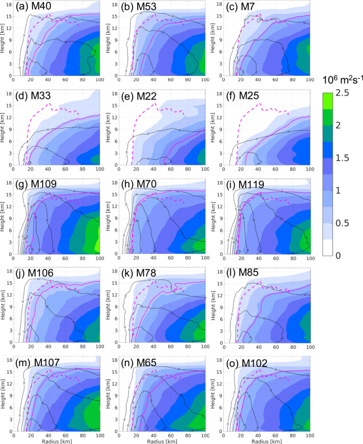
(a–l) The same as Figure 11 but for vertical cross‐section of azimuthally averaged tangential wind (contours) and absolute angular momentum (shading, Mm denoted by solid magenta line). (m–o) Three best members selected according to ε V10 ranking. The dash magenta lines are the reference Mms profile from spline analysis at mesoscale utilizing radar and aircraft instrumentation analysis. The member number is on the upper‐left corner of seach panel.
By plotting all the Mm surfaces together (Figure 13a), the wide range of the Mm surface structures shows up. As shown in DesRosiers et al. (2022) that the slope of the inner‐core absolute angular momentum surface is closely related to the TC development stages, this wide range of Mm surfaces in Figure 13a could exhibit various development stages of the ensemble members. The radial spread of the Mm surfaces at the mid‐to upper‐levels is much larger than that at lower levels. The stronger members have Mm surfaces closer to the center and are more vertical. Among the 120 Mm surfaces, two stand out for their good fit with Mms up to 15 km height. These two members are M70 and M119 (two solid magenta lines in Figure 13) shown in Figures 11h–11i and Figures 12h–12i. To better visualize the radial structure of the members, we also plotted the corresponding radial profiles of the azimuthally averaged tangential wind and absolute angular momentum at z = 1.6 km (Figures 13b and 13c). It can be seen from Figure 13b that the tangential wind outside the RMW from the SAMURAI analysis is within the range of the members. However, the tangential wind inside the RMW from the SAMURAI analysis is stronger than almost all the members. The same is observed in the radial structure of the absolute angular momentum (Figure 13c). The expected consequence is that the majority of the members will be below the observed intensity due to the radial structures shown in Figure 13c given that the intensification of the inner‐core tangential wind is associated with the horizontal advection of larger angular momentum inward according to the axisymmetric absolute angular momentum equation in the boundary layer. The two best members (M70 and M119) turn out to be the ones with all three profiles closest to the SAMURAI analysis, and also have some of the lowest errors compared to best track pressure.
Figure 13.

Forecast results from both CNTL and with‐tropical cyclone intensity at 1800 UTC 22 October 2015. (a) Azimuthally average angular momentum surfaces that intersect the radius of maximum wind at 1.6‐km height; (b) radial profiles of tangential wind at 1.6‐km height; (c) radial profiles of absolute angular momentum at 1.6 km height. All profiles are color coded by the ranking in Figure 9a. The dash magenta lines are the reference profiles from SAMURAI analysis. The solid magenta lines are M70 and M119.
To further analyze the member‐wise vertical structure, we also calculated the mean Mm heights between RMW and 75 km radius, and plot them against the maximum tangential winds (Figure 14a) and RMWs (Figure 14b) calculated at z = 1.6 km which is above the boundary layer. A radius of 75 km is selected in order to compare the simulation results to the SAMURAI result (Figure 10b) which extends to 75‐km radius. The mean Mm height has a wide distribution from ∼4 km (M25) up to ∼14 km (M70 and M119). The CNTL members generally have smaller mean Mm height values than the With‐TCI members, which can be attributed to the more slantwise Mm surfaces in CNTL members. The correlation between mean Mm heights and Vmax is 0.704, which indicates that the more intense TCs have more vertical Mm surfaces that reach a higher altitude. The negative correlation between mean Mm heights and RMW has a higher value (−0.8031), which indicates that the members with larger radius tend to have more slantwise Mm surfaces (consistent with Stern & Nolan, 2009). The mean Mm height from the SAMURAI analysis is slightly lower than the values of the best two members (M70 and M119) due to the wavy structure in the outflow region (Figure 10b). The best two members (M70 and M119) are always around the SAMURAI analysis, while M109 has a larger Vmax together with a larger RMW leading to a much larger Mm.
Figure 14.

Mean Mm height plotted against (a) maximum 10 m wind; (b) radius of maximum wind at 1.6 km height. The dash lines are the values from the spline analysis at mesoscale utilizing radar and aircraft instrumentation analysis. The two best members (M70 and M119) are denoted by hollow triangles while M109 is denoted by a hollow circle. The mean Mm height is calculated between radius of the maximum wind at z = 1.6 and 75 km radius.
In Figure Figures 11, 12 and 12a–12l, the bad members show larger RMWs and weaker wind fields while the good members have smaller RMWs and stronger wind fields in general. This indicates that the delayed development (contraction of the RMW) would be one of the forecast error sources. If the only variability in the ensemble was related to the timing of evolution, one would expect the correlation between RMW and intensity to be quite high since TCs start intensification with RMW contractions. However, the relatively low correlation between RMW and minimum sea level pressure (less than 0.6 all the time, not shown) suggests there are other error sources besides the delayed development. From Figures 13b and 14, intense members with large RMWs (hence large Mm) and weak members with small RMWs (hence small Mm) in the ensemble are observed. Tao et al. (2020) showed that the Mm value has a long memory of structure such that TCs with larger Mm tends to keep larger Mm during the development stage. This indicates another error source associated with the storm size, which could be identified from the Mm evolution.
To illustrate the member evolutions in a phase diagram, the time series of the maximum tangential winds and RMWs are plotted in the context of Mm isolines (Figure 15). Assume that M70 and M119 are the two members closest to the true evolution, and use them as references (magenta lines) for the comparisons. It is seen that there are some members with evolution pathways distributed near the reference lines of M70 and M119 in both CNTL and With‐TCI but the evolutions of these members are lagged in time with weaker intensity at the validation time (circles in Figure 15a). These members are the ones having delayed development stages.
Figure 15.

The evolution of Vmax and radius of the maximum wind at z = 1.6 km for (a) M1‐M60 from CNTL and (b) M61‐M120 from with‐tropical cyclone intensity from 2100 UTC 21 October 2015 to 0000 UTC 23 October 2015. The magenta lines are for the two best members (M70 and M119). The green line in each panel indicates the ensemble mean of the set. The black cross is for the spline analysis at mesoscale utilizing radar and aircraft instrumentation analysis at 1800 UTC 22 October 2015. Gray lines are contours of absolute angular momentum (0.2 × 10⁶ m2/s interval) calculated using the mean Coriolis parameter of all the members. The triangles indicate 0000 UTC 22 October 2015 while the circles indicate 1800 UTC 22 October 2015 for each member.
We can observe that the members in CNTL (Figure 15a) spread mostly below the reference lines of M70 and M119 with smaller Mm, and none of the members are of the same intensity as the two reference members at the validation time (circles in Figure 15a). In the set of With‐TCI (Figure 15b), the members tend to be about the same magnitude or larger than the Mm of the reference M70 and M119 and several members reach or exceed the intensity of M70 and M119 at the validation time (circles in Figure 15b). One important point to mention here is that some of the members reaching the reference intensity (darker blue color lines with smaller ε slp , M109 is among them) are away from the refence members, which means although these members have a good agreement with the best track in intensity, their RMWs and hence structures are not correct. This again shows that a single metric, even using minimum sea level pressure, may not capture the correct structural information. These members with smaller or larger Mm do not track the same evolution path in the phase space as M70 and M119 as they keep evolving on smaller Mm path or larger Mm path after the initial adjustment period. This finding implies that storms with different Mm are most likely different storms with different evolution pathways, which means it is impossible to obtain the same structure as the reference TC no matter how it subsequently develops. This storm size error in terms of Mm has not been well discussed in previous studies.
From Figure 15, we find that the evolution pathways of the members are significantly different in CNTL and With‐TCI. Assimilating the additional inner‐core observations from TCI in DA cycles generally increase the vortex strengths of the initial conditions. This improvement in the wind strength and structure corrects the timing of the entire TC evolution, such that the vortices are more advanced in With‐TCI compared to the ones in CNTL.
4. Conclusions and Discussion
In this study, we investigate the forecasted Patricia structure difference according to the minSLP error magnitudes in the peak RI stage. A wide range of intensification scenarios are obtained through two sets of ensemble forecasts initialized with and without assimilating the TCI data prior to the RI onset. Though the environment is favorable for intensification, the practical predictability of RI is directly related to the initial horizontal and vertical structure of the TC. The findings have practical implications as Hurricane Patricia (2015) is an extreme case under a nearly ideal development environment. Its close‐to‐ideal environment and vortex development act as a transition from pure ideal simulations to complicated real cases. The analysis and diagnostics in this study provide a valuable addition to the research of the relationship between a TC's structure and its subsequent evolution.
The analysis in Section 3.4 shows that through correcting the initial vortex structure only and without modifying model physics, the WRF model is capable of capturing the extreme development of Patricia (M70 and M119). We find significant differences in the angular momentum surfaces that intersect the radius of maximum wind among the members. For all the parameters analyzed, the two best members (M70 and M119) are the ones closest to the observed analysis, which confirms the importance of the TC's vertical and radial structures in the subsequent development. This importance of accurately specifying the radial structure is demonstrated to determine the intensification potential since the inner‐core intensification is the result of the radial inward advection of the larger angular momentum. This intensification goes hand in hand with the vertical structure evolution. Through detailed comparison of the structure‐related parameters, we discussed two intensification error sources: one is due to shifted development in the time, and the other is from a totally different storm such that no matter how the vortex develops, it is impossible to get the correct structure. For the error coming from the delayed contraction, one would expect the storm to have the same intensity and RMW as the observations if it were allowed to develop for more time, which is the same evolution path but shifted in time. The other error is that no matter how the storm develops, there is no point in time that the structure can be the same as the observations. The comparison of the selected best members according to minimum sea level pressure and maximum wind respectively shows that minimum sea level pressure acts better than maximum wind in evaluating the overall model performance which includes predicting the TC structure. However, there is still a false selection (M109) due to the possibility of getting a similar pressure drop at the TC center from different tangential wind profiles. This result indicates that traditional evaluation metrics using a point metric like intensity may not be sufficient to fully evaluate the performance of a TC forecast. A more holistic evaluation metric with the radial (e.g., RMW together with R17) and vertical (e.g., vertical RMW or Mm slope) structures of the vortex in addition to the intensity should be considered if the data are available.
The differences between the two ensemble sets mainly evolve from the initial vortex structures such that a deeper and stronger vortex intensifies earlier, and the evolution is closer to the observed evolution. Through the comparison between the initial conditions, we conclude that the assimilation of the TCI observations can correct the vertical structure of vortex in both primary and secondary circulations. Additional sensitivity experiments of assimilating different types of observations are also performed to evaluate the effect of different observation types/sources. The radar radial velocity mainly has an impact on the primary circulation in this Patricia case, while the wind data from the deep‐layer dropsondes can improve the primary circulation at all levels as well as the secondary circulation in the inflow region. On the contrary, the temperature and mixing ratio data from the deep‐layer dropsondes mostly affect the upper‐level thermodynamic structures and outflow strength. These findings from this study can provide suggestions for the future field campaign design as well as data‐assimilation strategies for operational forecasts.
Acknowledgments
D. Tao and M. Bell are supported by Office of Naval Research awards N000141613033 and N000142012069. P.J. van Leeuwen is supported by H2020 European Research Council project CUNDA award 694509. Y. Ying is supported by the Advanced Study Program in the National Center for Atmospheric Research which is a major facility sponsored by the National Science Foundation under Cooperative Agreement 1852977. We would like to thank Dr. Jonathan Martinez for providing the Spline Analysis at Mesoscale Utilizing Radar and Aircraft Instrumentation analysis and Dr. Robert Nystrom for the help on setting up the simulations. We also want to thank the three anonymous reviewers for the helpful comments. Computing was conducted on Supercomputer Stampede2 of the Texas Advanced Computing Center (TACC) and on Supercomputer Cheyenne of the National Center for Atmospheric Research (NCAR).
Tao, D. , van Leeuwen, P. J. , Bell, M. , & Ying, Y. (2022). Dynamics and predictability of tropical cyclone rapid intensification in ensemble simulations of Hurricane Patricia (2015). Journal of Geophysical Research: Atmospheres, 127, e2021JD036079. 10.1029/2021JD036079
Data Availability Statement
The conventional observations are available on NCAR RDA: https://doi.org/10.5065/9235-WJ24. The TCI dropsonde data can be downloaded at https://data.eol.ucar.edu/dataset/488.004. The TCI radar data can be downloaded at https://www.aoml.noaa.gov/hrd/Storm_pages/patricia2015/radar.html. The PSU EnKF code can be downloaded at http://adapt.psu.edu/index.php?loc=outreach. The tangential and radial winds from the two ensemble sets as well as the SAMURAI analysis used in this paper are available on Zenodo: https://doi.org/10.5281/zenodo.6366545.
References
- Aircraft Operations Center . (2016). Tropical cyclone operations: Challenges in 2015; new products and services planned for 2016 and 2017. NOAA Office of Marine and Aviation Operations. Retrieved from https://www.icams-portal.gov/meetings/TCORF/ihc16/2016presentations.html [Google Scholar]
- Aksoy, A. , Cione, J. J. , Dahl, B. A. , & Reasor, P. D. (2022). Tropical cyclone data assimilation with Coyote uncrewed aircraft system observations, very frequent cycling, and a new online quality control technique. Monthly Weather Review, Early online release. 10.1175/MWR-D-21-0124.1 [DOI] [Google Scholar]
- Barker, D. M. , Huang, W. , Guo, Y. R. , Bourgeois, A. , & Xiao, Q. (2004). A three‐dimensional variational data assimilation system for MM5: Implementation and initial results. Monthly Weather Review, 132, 897–914. [DOI] [Google Scholar]
- Bell, M. , & coauthors. (2016). ONR tropical cyclone intensity 2015 NASA WB‐57 HDSS dropsonde data. Version 1.0. [Dataset]. UCAR/NCAR—Earth Observing Laboratory. 10.5065/D6KW5D8M [DOI] [Google Scholar]
- Bell, M. M. , Montgomery, M. T. , &, Emanuel, K. A. (2012). Air–sea enthalpy and momentum exchange at major hurricane wind speeds observed during CBLAST. Journal of the Atmospheric Sciences, 69, 3197–3222. 10.1175/JAS-D-11-0276.1 [DOI] [Google Scholar]
- Biondi, R. , Ho, S.‐P. , Randel, W. , Syndergaard, S. , & Neubert, T. (2013). Tropical cyclone cloud‐top height and vertical temperature structure detection using GPS radio occultation measurements. Journal of Geophysical Research: Atmospheres, 118, 5247–5259. 10.1002/JGRD.50448 [DOI] [Google Scholar]
- Carrasco, C. , Landsea, C. , & Lin, Y. (2014). The influence of tropical cyclone size on its intensification. Weather and Forecasting, 29, 582–590. 10.1175/WAF-D-13-00092.1 [DOI] [Google Scholar]
- Christophersen, H. , Aksoy, A. , Dunion, J. , & Sellwood, K. J. (2017). The impact of NASA Global Hawk unmanned aircraft dropwindsonde observations on tropical cyclone track, intensity, and structure: Case studies. Monthly Weather Review, 145, 1817–1830. 10.1175/MWR-D-16-0332.1 [DOI] [Google Scholar]
- Christophersen, H. , Atlas, R. , Aksoy, A. , & Dunion, J. (2018). Combined use of Satellite observations and Global Hawk unmanned aircraft Dropwindsondes for improved tropical cyclone analyses and forecasts. Weather and Forecasting, 33, 1021–1031. 10.1175/WAF-D-17-0167.1 [DOI] [Google Scholar]
- DesRosiers, A. , Bell, M. M. , & Cha, T.‐Y. (2022). Vertical vortex development of Hurricane Michael (2018) during rapid intensification. Monthly Weather Review. 150, 99–114. 10.1175/MWR-D-21-0098.1 [DOI] [Google Scholar]
- Elsberry, R. L. , Lambert, T. D. B. , & Boothe, M. A. (2007). Accuracy of Atlantic and eastern North Pacific tropical cyclone intensity forecast guidance. Weather and Forecasting, 22, 747–762. 10.1175/WAF1015.1 [DOI] [Google Scholar]
- Emanuel, K. (2012). Self‐stratification of tropical cyclone outflow. Part II: Implications for storm intensification. Journal of the Atmospheric Sciences, 69, 988–996. 10.1175/JAS-D-11-0177.1 [DOI] [Google Scholar]
- Feng, J. , & Wang, X. (2019). Impact of assimilating upper‐level dropsonde observations collected during the TCI field campaign on the prediction of intensity and structure of Hurricane Patricia (2015). Monthly Weather Review, 147, 3069–3089. 10.1175/MWR-D-18-0305.1 [DOI] [Google Scholar]
- Foerster, A. M. , & Bell, M. M. (2017). Thermodynamic retrieval in rapidly rotating vortices from multiple‐Doppler radar data. Journal of Atmospheric and Oceanic Technology, 34, 2353–2374. 10.1175/JTECH-D-17-0073.1 [DOI] [Google Scholar]
- Foerster, A. M. , Bell, M. M. , Harr, P. A. , & Jones, S. C. (2014). Observations of the eyewall structure of Typhoon Sinlaku (2008) during the transformation stage of extratropical transition. Monthly Weather Review, 142, 3372–3392. 10.1175/MWR-D-13-00313.1 [DOI] [Google Scholar]
- Fox, K. R. , & Judt, F. (2018). A numerical study on the extreme intensification of Hurricane Patricia (2015). Weather and Forecasting, 33, 989–999. 10.1175/WAF-D-17-0101.1 [DOI] [Google Scholar]
- Hendricks, E. A. , Peng, M. S. , Fu, B. , & Li, T. (2010). Quantifying environmental control on tropical cyclone intensity change. Monthly Weather Review, 138, 3243–3271. 10.1175/2010MWR3185.1 [DOI] [Google Scholar]
- Jiménez, P. A. , Dudhia, J. , González‐Rouco, J. F. , Navarro, J. , Montávez, J. P. , & García‐Bustamante, E. (2012). A Revised scheme for the WRF surface layer formulation. Monthly Weather Review, 140, 898–918. 10.1175/MWR-D-11-00056.1 [DOI] [Google Scholar]
- Klotzbach, P. J. , Bell, M. M. , Bowen, S. G. , Gibney, E. J. , Knapp, K. R. , & Schreck, C. J. III . (2020). Surface pressure a more skillful predictor of normalized hurricane damage than maximum sustained wind. Bulletin of the American Meteorological Society, 101, E830–E846. 10.1175/BAMS-D-19-0062.1 [DOI] [Google Scholar]
- Koteswaram, P. (1967). On the structure of hurricanes in the upper troposphere and lower stratosphere. Monthly Weather Review, 95, 541–564. [DOI] [Google Scholar]
- Kren, A. C. , Cucurull, L. , & Wang, H. (2018). Impact of UAS Global Hawk dropsonde data on tropical and extratropical cyclone forecasts in 2016. Weather and Forecasting, 33, 1121–1141. 10.1175/WAF-D-18-0029.1 [DOI] [Google Scholar]
- Lu, X. , & Wang, X. (2019). Improving hurricane analyses and predictions with TCI, IFEX field campaign observations, and CIMSS AMVs using the advanced hybrid data assimilation system for HWRF. Part I: What is missing to capture the rapid intensification of Hurricane Patricia (2015) when HWRF is already initialized with a more realistic analysis? Monthly Weather Review, 147, 1351–1373. 10.1175/MWR-D-18-0202.1 [DOI] [Google Scholar]
- Lu, X. , & Wang, X. (2020). Improving Hurricane analyses and predictions with TCI, IFEX field campaign observations, and CIMSS AMVs using the advanced Hybrid data assimilation system for HWRF. Part II: Observation impacts on the analysis and prediction of Patricia (2015). Monthly Weather Review, 148, 1407–1430. 10.1175/MWR-D-19-0075.1 [DOI] [Google Scholar]
- Martinez, J. , Bell, M. M. , Rogers, R. F. , & Doyle, J. D. (2019). Axisymmetric potential vorticity evolution of Hurricane Patricia (2015). Journal of the Atmospheric Sciences, 76, 2043–2063. 10.1175/JAS-D-18-0373.1 [DOI] [Google Scholar]
- Nystrom, R. G. , & Zhang, F. (2019). Practical uncertainties in the limited predictability of the record‐breaking intensification of Hurricane Patricia (2015). Monthly Weather Review, 147, 401–423. 10.1175/MWR-D-18-0450.1 [DOI] [Google Scholar]
- Qin, N. , & Zhang, D.‐L. (2018). On the extraordinary intensification of Hurricane Patricia (2015). Part I: Numerical experiments. Weather and Forecasting, 33, 1205–1224. 10.1175/WAF-D-18-0045.1 [DOI] [Google Scholar]
- Rivoire, L. , Birner, T. , & Knaff, J. A. (2016). Evolution of the upper‐level thermal structure in tropical cyclones. Geophysical Research Letters, 43, 10530–10537. 10.1002/2016gl070622 [DOI] [Google Scholar]
- Rogers, R. , Aberson, S. , Bell, M. M. , Cecil, D. J. , Doyle, J. D. , Kimberlain, T. B. , et al. (2017). Rewriting the tropical record books: The extraordinary intensification of Hurricane Patricia (2015). Bulletin of the American Meteorological Society, 98, 2091–2112. 10.1175/BAMS-D-16-0039.1 [DOI] [Google Scholar]
- Skamarock, W. C. , & Coauthors. (2008). A description of the advanced research WRF version 3. NCAR Tech. Note NCAR/TN‐4751STR, 113 pp. 10.5065/D68S4MVH [DOI] [Google Scholar]
- Stern, D. P. , & Nolan, D. S. (2009). Reexamining the vertical structure of tangential winds in tropical cyclones: Observations and theory. Journal of the Atmospheric Sciences, 66, 3579–3600. 10.1175/2009jas2916.1 [DOI] [Google Scholar]
- Tao, D. , Bell, M. M. , Rotunno, R. , & van Leeuwen, P. J. (2020). Why do the maximum intensities in modeled tropical cyclones vary under the same environmental conditions? Geophysical Research Letters, 47, e2019GL085980. 10.1029/2019gl085980 [DOI] [Google Scholar]
- Tao, D. , & Zhang, F. (2019). Evolution of dynamic and thermodynamic structures before and during rapid intensification of tropical cyclones: Sensitivity to vertical wind shear. Monthly Weather Review, 147, 1171–1191. 10.1175/MWR-D-18-0173.1 [DOI] [Google Scholar]
- Weng, Y. , & Zhang, F. (2012). Assimilating airborne Doppler radar observations with an ensemble Kalman filter for convection‐permitting hurricane initialization and prediction: Katrina (2005). Monthly Weather Review, 140, 841–859. 10.1175/2011MWR3602.1 [DOI] [Google Scholar]
- Weng, Y. , & Zhang, F. (2016). Advances in convection‐permitting tropical cyclone analysis and prediction through EnKF assimilation of reconnaissance aircraft observations. Journal of the Meteorological Society of Japan, 94, 345–358. 10.2151/jmsj.2016-018 [DOI] [Google Scholar]
- Wick, G. A. , Dunion, J. P. , Black, P. G. , Walker, J. R. , Torn, R. D. , Kren, A. C. , et al. (2020). NOAA’s sensing Hazards with operational unmanned technology (SHOUT) experiment observations and forecast impacts. Bulletin of the American Meteorological Society, 101, E968–E987. 10.1175/BAMS-D-18-0257.1 [DOI] [Google Scholar]
- Xu, J. , & Wang, Y. (2015). A statistical analysis on the dependence of tropical cyclone intensification rate on the storm intensity and size in the North Atlantic. Weather and Forecasting, 30, 692–701. 10.1175/WAF-D-14-00141.1 [DOI] [Google Scholar]
- Xu, J. , & Wang, Y. (2018). Effect of the initial vortex structure on intensification of a numerically simulated tropical cyclone. Journal of the Meteorological Society of Japan, 96, 111–126. 10.2151/jmsj.2018-014 [DOI] [Google Scholar]
- Yamada, H. , Ito, K. , Tsuboki, K. , Shinoda, T. , Ohigashi, T. , Yamaguchi, M. , et al. (2021). The double warm‐core structure of Typhoon Lan (2017) as observed through the first Japanese eyewall‐penetrating aircraft reconnaissance. Journal of the Meteorological Society of Japan, 99. 10.2151/jmsj.2021-063 [DOI] [Google Scholar]
- Zawislak, J. , Rogers, R. F. , Aberson, S. D. , Alaka, G. J. , Alvey, G. , Aksoy, A. , et al. (2022). Accomplishments of NOAA’S airborne hurricane field program and a broader future approach to forecast improvement. Bulletin of the American Meteorological Society, 103, E311–E338. 10.1175/BAMS-D-20-0174.1 [DOI] [Google Scholar]
- Zhang, F. , Snyder, C. , & Sun, J. (2004). Impacts of initial estimate and observation availability on convective‐scale data assimilation with an ensemble Kalman filter. Monthly Weather Review, 132, 1238–1253. [DOI] [Google Scholar]
- Zhang, F. , & Weng, Y. (2015). Predicting hurricane intensity and associated hazards: A five‐year real‐time forecast experiment with assimilation of airborne Doppler radar observations. Bulletin of the American Meteorological Society, 96, 25–33. 10.1175/bams-d-13-00231.1 [DOI] [Google Scholar]
- Zhang, F. , Weng, Y. , Gamache, J. F. , & Marks, F. D. (2011). Performance of cloud‐resolving hurricane initialization and prediction during 2008–2010 with ensemble data assimilation of inner‐ core airborne Doppler radar observations. Geophysical Research Letters, 38, L15810. 10.1029/2011GL048469 [DOI] [Google Scholar]
- Zhang, F. , Weng, Y. , Sippel, J. A. , Meng, Z. , & Bishop, C. H. (2009). Cloud‐resolving hurricane initialization and prediction through assimilation of Doppler radar observations with an ensemble Kalman filter. Monthly Weather Review, 137, 2105–2125, 10.1175/2009MWR2645.1 [DOI] [Google Scholar]
- Zhang, Y. J. , Meng, Z. , Weng, Y. , & Zhang, F. (2014). Predictability of tropical cyclone intensity evaluated through 5‐yr forecasts with a convection‐permitting regional‐scale model in the Atlantic Basin. Weather and Forecasting, 29, 1003–1023. 10.1175/WAF-D-13-00085.1 [DOI] [Google Scholar]
Associated Data
This section collects any data citations, data availability statements, or supplementary materials included in this article.
Data Availability Statement
The conventional observations are available on NCAR RDA: https://doi.org/10.5065/9235-WJ24. The TCI dropsonde data can be downloaded at https://data.eol.ucar.edu/dataset/488.004. The TCI radar data can be downloaded at https://www.aoml.noaa.gov/hrd/Storm_pages/patricia2015/radar.html. The PSU EnKF code can be downloaded at http://adapt.psu.edu/index.php?loc=outreach. The tangential and radial winds from the two ensemble sets as well as the SAMURAI analysis used in this paper are available on Zenodo: https://doi.org/10.5281/zenodo.6366545.