Multiscale characterization of pathological bone tissue

ABSTRACT

Bone is a complex natural material with a complex hierarchical multiscale organization, crucial to perform its functions. Ultrastructural analysis of bone is crucial for our understanding of cell to cell communication, the healthy or pathological composition of bone tissue, and its three‐dimensional (3D) organization. A variety of techniques has been used to analyze bone tissue. This article describes a combined approach of optical, scanning electron, and transmission electron microscopy for the ultrastructural analysis of bone from the nanoscale to the macroscale, as illustrated by two pathological bone tissues. By following a top‐down approach to investigate the multiscale organization of pathological bones, quantitative estimates were made in terms of calcium content, nearest neighbor distances of osteocytes, canaliculi diameter, ordering, and D‐spacing of the collagen fibrils, and the orientation of intrafibrillar minerals which enable us to observe the fine structural details. We identify and discuss a series of two‐dimensional (2D) and 3D imaging techniques that can be used to characterize bone tissue. By doing so we demonstrate that, while 2D imaging techniques provide comparable information from pathological bone tissues, significantly different structural details are observed upon analyzing the pathological bone tissues in 3D. Finally, particular attention is paid to sample preparation for and quantitative processing of data from electron microscopic analysis.

Multiscale characterization of pathological bone tissues.

1. INTRODUCTION

Bone tissue affected by pathological conditions undergoes alterations (Bishop, 2016; Boskey et al., 2017), of which the precise nature and its mechanical consequences are still to be revealed. Considering the fact that the hierarchical organization of healthy bone is still under debate (Mitchell & Van Heteren, 2016), determining the structures and motifs in pathological bone needs to be dealt with at all hierarchical levels and should address as many aspects of the structure as possible. A considerable amount of literature has been published concerning the hierarchical organization of bone (Boskey & Robey, 2018; Cressey & Cressey, 2003; Grandfield, Vuong, & Schwarcz, 2018; McNally, Nan, Botton, & Schwarcz, 2013; McNally, Schwarcz, Botton, & Arsenault, 2012; Reznikov, Bilton, Lari, Stevens, & Kröger, 2018; Schwarcz, 2015; Shah, Ruscsák, & Palmquist, 2019). These studies show that bone is a composite material, with mineralized type I collagen fibril being the basic structural unit (Weiner & Wagner, 1998). Type I collagen fibrils, acting as a template for mineralization during bone formation, non‐collagenous proteins, and calcium phosphate in the form of plate‐like shaped carbonated hydroxyapatite crystals, collectively organized in a hierarchical way, are responsible for the mechanical properties of bone (Reznikov, Shahar, & Weiner, 2014a). The hierarchical organization of bone starts at the nanolevel and extends all the way up to the macrolevel providing a framework responsible for its mechanical stiffness and strength and subsequent functioning (Reznikov et al., 2014a). Severe clinical consequences (Marini et al., 2007; Marini et al., 2017; Van Dijk & Sillence, 2014) may arise as a result of any alteration in the hierarchical (nanoscale to macroscale) organization of bone.

Osteogenesis imperfecta (OI), also known as “brittle bone disease,” is an inherited bone disease in which alteration of a single mutation in the collagen type I gene leads to bone fragility with severe clinical consequences. The clinical manifestations vary widely between the different types of OI ranging from patients who have mild symptoms with a normal life expectancy to intrauterine death (Kivirikko, 1993; Nijhuis et al., 2019; Prockop, 1990; Thomson, 1927). The majority of the OI population have an autosomal dominant inheritance leading to OI types I to IV due to a mutation in the COL1A1 or COL1A2 gene. These genetic defects, changing only one amino acid in collagen molecules, have an impact on bone structure from the nanoscale to the millimeter and whole bone level (Van Dijk et al., 2011). The molecular structure of collagen molecules changes dramatically in such pathological conditions, that is, the diameter of type I collagen fibrils in OI bone is smaller (Cassella, Barber, Catterall, & Ali, 1994; Eimar et al., 2016; Kłosowski et al., 2017; Sarathchandra, Pope, & Ali, 1999), and the collagen forms more wavy structures compared with its healthy counterpart, which might affect the packing of the collagen molecules at the fibril level (Gjaltema & Bank, 2017; Li et al., 2016). In OI bone abnormally high matrix mineralization is found independent of the mutation type. Fratzl‐Zelman et al. found a similar crystal size in the bone of OI type I compared with normal bone but the relative mineral volume fraction was increased by 12% due to a larger number of crystals in the same matrix volume (Fratzl‐Zelman et al., 2014).

Throughout history, polarized optical microscopy (POM) has been widely used in order to determine the structure of collagen not only in bone tissues but also in other biological tissues (Boyde & Riggs, 1990; Bromage et al., 2003; Gebhardt, 1905; Wolman & Kasten, 1986). In POM, layers of collagen fiber bundles are typically visible with well‐organized alternating light and dark layers due to the birefringence of collagen. The applications of POM in the field of bone research provided crucial insights into the hierarchical organization of bone tissue. Possibly the researcher that comes to mind is Walter Gebhardt who predominantly employed optical microscopy to identify the elements of bone architecture and published his findings in 1905 in which he proposed the simplest model of bone structure (Gebhardt, 1905). His findings can still be validated till this day by scientists who demonstrate alternating layers of collagen fibers visible using POM. Moreover, it has been argued that collagen fiber orientation can also be determined by employing POM (Rieppo et al., 2008), however, it is extremely crucial to preserve the same thickness of the sections in thin‐section sample preparation during microtomy. The detailed explanation of the historical findings of bone organization made by POM is clearly beyond the scope of this article, however, it is important to mention that several scientists have different views in terms of the structure of bone tissue. The orthogonal plywood model based on Gebhardt initially paved the way for models of bone tissue which assume two distinct orientations of lamellae. Later the twisted plywood model was proposed by Weiner, Traub, and Wagner (1999) and Wagermaier et al. (2006) which contains sub‐layers of lamellae maintaining specific orientations that changes angle within the motif. Similar models were proposed by Varga et al. (2013) and Schrof, Varga, Galvis, Raum, and Masic (2014) both models containing the twisted plywood motif but with a smoother transition from one orientation of collagen fibers to another. Moreover, Reznikov et al. (Reznikov, Almany‐Magal, Shahar, & Weiner, 2013; Reznikov, Shahar, & Weiner, 2014b) proposed a model similar to that proposed by Weiner et al. (1999), illustrating three different sub‐layers namely, fanning, disordered, and unidirectional motifs.

Other techniques, such as atomic force microscopy (AFM), scanning electron microscopy (SEM), and transmission electron microscopy (TEM), have been used to identify the nanolevel hierarchy of bone tissue (Boivin, Anthoine‐Terrier, & Obrant, 1990; Hassenkam et al., 2004; Keene & Tufa, 2010; McNally et al., 2013; Shah et al., 2019). An important aspect of AFM is that it can also be utilized as a nanoindentation tool to measure mechanical properties of bone tissue (Lefèvre, Guivier‐Curien, Pithioux, & Charrier, 2013; Wallace, 2012). However, the major drawback of AFM compared with other techniques is that it provides only two‐dimensional (2D) information on the organization of bone tissue. Therefore, in bone research, AFM is mainly used to determine the mechanical properties of bone. However, it is also important to mention that AFM, similarly to TEM, has been employed to investigate the nanolevel features of bone tissues such as the size of the minerals (Eppell, Tong, Lawrence Katz, Kuhn, & Glimcher, 2001; Tong, Glimcher, Katz, Kuhn, & Eppell, 2003) and characteristic of collagen fibrils [D‐spacing (Erickson et al., 2013) and diameter (Habelitz, Balooch, Marshall, Balooch, & Marshall, 2002)]. Electron microscopy techniques are possibly the most widely used techniques to identify the structural details of bone tissue after POM. For instance, conventional SEM provides nanometer resolution of the sample surface and it is also a useful tool to scan the whole surface of the sample, providing information over hundreds of micrometers. Moreover, conventional TEM has also allowed for local assessment of the nanolevel structural hierarchy of bone (Rubin et al., 2003) and has been used to gain important insights through investigations of the shape and size of minerals (Reznikov et al., 2018; Weiner & Traub, 1989), arrangements of minerals with collagen fibrils (Su, Sun, Cui, & Landis, 2003; Weiner, Arad, & Traub, 1991), and characteristic 67 nm D‐spacing of collagen fibril (Deshpande & Beniash, 2008). However, all this information has been acquired in two dimensions only.

Investigations of these abovementioned ultrastructural features require detailed three‐dimensional (3D) high‐resolution imaging of the nanostructure and microstructure of the bone tissue. The acquisition of high‐resolution 3D images and elucidation of the ultrastructural organization of bone tissue provides information for future studies, helps to collect data for quantitative analysis from multiple length scales, and ultimately may lead identification of new treatments. To date, several imaging tools have been used in bone community to reveal the true features of healthy and pathological bone tissues (Georgiadis, Müller, & Schneider, 2016). Among many other tools, electron microscopy techniques, including TEM (Boivin et al., 1990; Keene & Tufa, 2010) and SEM (Georgiadis et al., 2016), offer high spatial resolution and can potentially provide images on multiple length scales, although the acquired images are inherently 2D. To overcome this drawback, advanced electron microscopy techniques, such as focused ion beam‐serial slice and view (FIB‐SSV) for SEM and electron tomography (ET) for TEM, can be employed. While FIB‐SSV involves sequential milling and subsequent imaging of freshly exposed surfaces, ET depends on tilting of approximately 100 nm thick samples by, say, ±70° and thereafter reconstructing the 3D structure from the images obtained. Moreover, FIB‐SSV and ET are somewhat complementary techniques due to their inherent advantages and disadvantages. For instance, the resulting images from ET resolve details at high spatial resolution but are restricted to smaller volumes, while the images for FIB‐SSV resolve details at a lower spatial resolution but provides information for much larger volumes. Therefore, SEM by employing FIB‐SSV and TEM by employing ET can be used profitably in the elucidation of the ultrastructure of healthy and pathological bone. Last but not least, techniques involving electron microscopes not only provide structural information of the bone tissue, but can also provide useful structural insights into other biological or synthetic materials such as biological exoskeletons (Rivera et al., 2020; Soleimani et al., 2020; Sun & Bhushan, 2012; Yao et al., 2010), biomimetic materials (Dede Eren et al., 2020; Mohammadi, Sesilja Aranko, Paul Landowski, Wagermaier, & Linder, 2019; Wegst, Bai, Saiz, Tomsia, & Ritchie, 2015), and implant materials (Linder et al., 1983; Mendonça, Mendonça, Aragão, & Cooper, 2008; Thorfve, Palmquist, & Grandfield, 2015).

The current understanding in the literature regarding structural alterations in pathological bone is mainly based on conventional techniques, such as histology and optical microscopy, that provide limited information for a complex 3D material and likely hinders full understanding of these complex biological materials (Shahar & Weiner, 2018). Therefore, a real 3D analysis of pathological bone tissues by using various microlevel to nanolevel techniques is needed. In this study we aim to demonstrate some of the possible conventional techniques, such as atomic absorption spectrometry (AAS) for determining the calcium content and POM for structural overview, and advanced techniques, such as EM tomography and FIB‐SSV SEM for structural details, that can be employed to reveal the ultrastructural characteristics of bone tissue. Hypothesizing that by focusing on bottom‐up and top‐down approaches one can build a “bridge” between the nanolevel hierarchy and microlevel structures. Unraveling the 3D structure and analyzing several aspects of the hierarchical organization of bone tissues can bring us one step closer toward understanding structure–function relations in bone.

2. MATERIALS AND METHODS

2.1. Sample collection

The present study was carried out on cortical bone tissue samples from surgical procedures, which was considered medical waste. This waste is normally disposed of and can be used for research purposes. According to the Central Committee on Research involving Human Subjects (CCMO), this type of study does not require approval from an ethics committee in the Netherlands (for full details, see Central Committee on Research Involving Human Subjects, 2021).

Bone tissue from the midshaft tibia of a 6‐year‐old patient with spondyloepiphyseal dysplasia congenital (SEDC) and bone tissue from the femur of an 8‐year‐old OI type IV (osteogenesis imperfecta) patient was used. Here it is important to emphasis that a close collaboration with medical doctors (physicians) is a key aspect in order to determine which bone tissues samples will be used in further experiments. The mutations causing the OI type IV bone and detailed information regarding the patients which were used in this study can be found in Appendix 1 and Table S1. SEDC is caused by a mutation in COL2A1 a gene that provides instructions for the production of the pro‐alpha1(II) chain of type II collagen which is found in the vitreous humor of the eye and cartilage. OI Type IV is caused by a mutation in COL1A2 gene where in position 754 there is a glycine substitution with serine. Both samples did not contain any fracture callus formation as assessed by X‐ray examination before surgery, as expected as surgery was performed for deformity and not for fractures.

2.2. Imaging techniques

SEM and TEM were used to reveal the structural features of two pathological bone tissues at multiple length scales from (μm/mm) material level to (nm) collagen fibril level. POM and SEM were employed to determine the density of osteocytes as well as to identify structural differences. Additionally, atomic absorption spectroscopy (AAS) was employed to determine the mineral content of these two pathological bone tissues and picrosirius red staining was used to identify the characteristic features of collagen fibers. Moreover, POM together with several image analysis tools was used to uncover the organizational differences for the osteocytes and as picrosirius red stains collagen, it was used to investigate orientation of collagen fibers. Three‐dimensional focused ion beam scanning electron microscopy (3D FIB/SEM) was used to determine the 3D structure of bone samples at the micrometer level using block‐face imaging in “slice and view mode.” Finally, electron tomography was used to determine the 3D structure of mineralized collagen fibrils at the nanometer level. As the focus of this article is on microscopy, results obtained from AAS and picrosirius staining are presented in Appendix 2.

Moreover, in order to identify the regions of interest (ROI), several important factors were considered depending on the level of hierarchy that was intended to be analyzed. While imaging the sections under POM (Figure 4) for which a total of 200 sections were analyzed, the most important structural elements that were considered as ROI were osteons, osteocytes, and at higher magnifications the lacunar canaliculi network. Upon determining the ROIs via POM, the in total 40 samples were used for SEM (20 for each sample) to identify the structural elements at different level of hierarchy. At this level of hierarchy, either the lacunar canaliculi network, the twisted plywood motif (Figure 8), the collagen fiber bundles (Figure 9) or collagen fibers were determined as ROI. Thereafter, by employing the FIB TEM lamellae preparation technique (in total four different thin slices were prepared by using both samples), we were able to prepare a thin slice from the ROI found via SEM. Finally, at the nanolevel of hierarchy, collagen fibrils (Figures 11, 12, 13) together with intrafibrillar minerals (Figures 14 and 15) were the focus of our interest and were identified as ROI.

FIGURE 4.

Normal optical microscopy images of (a) SEDC showing a single intact surface with clearly visible osteocytes (black dots) and (c) OI type IV bone showing separated small island‐like features. The same regions are shown in (b) and (d) using a polarizer. Scale bars: 100 μm

FIGURE 8.

Representative images of twisted plywood motif of (a–c) SEDC bone, (d–f) OI type IV bone

FIGURE 9.

Representative organizational motifs of (a,b) SEDC bone; (c,d) OI type IV bone. Cross‐sections of canaliculi are marked with a white arrow in (a) and (c). (b) and (d) correspond to highlighted yellow area in (a) and (c), respectively. Collagen fibrils that form a bundle‐like motif are marked with a light orange rectangle. Scale bars: 1 μm

FIGURE 11.

The 2D TEM images from SEDC bone in (a), (c), and (d) and OI type IV bone in (b), (e), and (f). The characteristic banding pattern of collagen fibrils is visible in all images. Yellow arrows indicate the intrafibrillar crystals. The black dots are gold nanoparticles used as fiducial markers for electron tomography and further reconstruction

FIGURE 12.

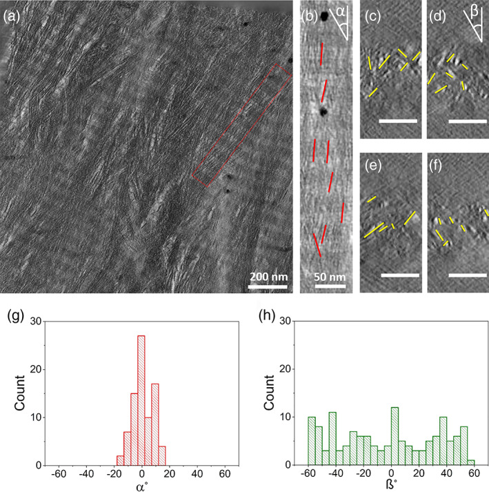
Electron tomography of SEDC bone. (a) The 2D projection of the top‐view tomographic reconstruction slices (100 z‐slices averaged) of the FIB thin section from SEDC bone. The red rectangle depicts the single collagen fibril shown in b). (b) Top‐view tomographic reconstruction slice of single collagen fibril. Crystals are highlighted with red lines. (c–f) Cross‐section reconstruction slice of one single collagen fibril. Crystals are highlighted with yellow lines. (g) Longitudinal and (h) lateral angular distribution of intrafibrillar crystals shown in (b–f), respectively. About 300 crystals, at least 20 nm apart for (g) and 100 nm apart for (h), were analyzed. Scale bars for (c–f): 50 nm

FIGURE 13.

Electron tomography of OI type IV bone. (a) 2D projection of the top‐view tomographic reconstruction slices (100 z‐slices averaged) of the FIB thin section from OI type IV bone. The red rectangle depicts the single collagen fibril shown in (b). (b) Top‐view tomographic reconstruction slice of single collagen fibril. Crystals are highlighted with red lines. (c–f) Cross‐section reconstruction slice of one single collagen fibril. Crystals are highlighted with yellow lines. (g) Longitudinal and (h) lateral angular distribution of intrafibrillar crystals shown in (b–f). About 300 crystals, at least 20 nm apart for (g) and 100 nm apart for (h), were analyzed. Scale bars for (c–f): 50 nm

FIGURE 14.

The 2D projection of the top‐view tomographic reconstruction slices (a–d) showing a single mineralized collagen fibril in OI Type IV bone. The defects in the mineralized collagen fibril are highlighted by yellow arrows. Regions with a stack of crystals and defects are marked with red and yellow rectangles, respectively. (e) The 2D projection of a cross‐section tomographic reconstruction slice showing a stack of crystals and (f) similarly for a defected region. Scale bars: 50 nm

FIGURE 15.

The 2D projection of the top‐view tomographic reconstruction slices (a–d) showing a single mineralized collagen fibril in SEDC bone. Regions with a stack of crystals and defects are marked with red rectangles. (e,f) The 2D projection of a cross‐section tomographic reconstruction slice showing a stack of crystals marked with a white circle. Scale bars: 50 nm

2.3. Sample preparation for optical and electron microscopy

Advanced electron microscopy techniques require multiple and meticulous sample preparation steps before they can be employed to characterize biological samples such as bone. Fixation, demineralization, staining, and embedding of the samples are discussed and for each step, the method and chemicals used are explained in detail in Figures S1–S5).

Thirty small pieces of bone tissues both from OI and SEDC (Appendix 3, Figure S6) were cut to approximately 2 mm × 2 mm × 2 mm. Thereafter bone pieces were immersed in a solution that contains 2% paraformaldehyde (PFA) and 5% ethylenediaminetetraacetic acid (EDTA) in a cacodylate buffer at pH 7 for 2 days. After this pre‐fixation and demineralization procedure the bone pieces were washed using double distilled water three times (twice for 6 hr and then once for 16 hr) on a rocking table to get rid of the residual EDTA (Full details can be found in Appendix S2). Thereafter, the samples were fixed again with 4% glutaraldehyde in a cacodylate buffer at pH 7 and washed with double distilled water in steps as indicated above. The fixation methods used have been shown in the literature (Bakker & Klein‐nulend, 2012; Boivin et al., 1990; Georgiadis et al., 2016; Keene & Tufa, 2010; Shah et al., 2019) to preserve the structure of bone therefore we do not have any indication as to why major structural defects might be observed due to sample preparation techniques.

The fixed and demineralized samples were stained with a procedure called OTOTO (Seligman, Wasserkrug, & Hanker, 1966) staining, also known as conductive staining. The OTOTO procedure relies on a sequential exposure of osmium tetroxide (Sigma‐Aldrich, CAS No: 20816‐12‐0) (O) and thiocarbohydrazide (Sigma‐Aldrich, CAS No: 2231‐57‐4) (T), which bind to the sample in a chain‐like manner (Seligman et al., 1966) and provides a better contrast as well as conductive properties, as elaborated in various studies (Reznikov et al., 2014b, 2018). The Epon embedding was carried out in several steps, each for 2 hr in 25% Epon resin + 75% acetone, 50% Epon resin + 50% acetone, 75% Epon resin + 25% acetone, and 100% Epon resin, respectively, which was followed by 100% Epon resin overnight and final embedding in a mold for 48 hr at 60 °C. After 48 hr, the embedded bone pieces were trimmed using a glass knife on a microtome to expose the embedded tissue. It may be worth to mention that the specimen size of 2 mm × 2 mm × 2 mm, which was on one side eventually trimmed down to an area of 2 mm × 2 mm × 5 μm by microtoming, resulted for cutting from macroscopic pieces of bone removed during surgery. As the mechanical stability of the samples which are used for SEM and FIB‐SSV is one of the most critical parameters in order to obtain reliable results for further analysis, an in‐house made sample holder (Figure 1) was used to provide the necessary stability during the SSV procedure. Together with the in‐house sample holder, bone samples were fixed by using a silver paste to position them as stable as possible under the electron and/or ion beam and reduce the charging effect.

FIGURE 1.

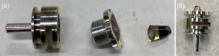
In‐house made sample holder for serial slice and view (SSV) characterization of trimmed blocks contacting bone pieces

2.3.1. Polarized optical microscopy

An axioplan (Zeiss) was used for POM characterization. The embedded bone pieces were used to prepare 5‐μm thick slices, which were cut with the microtome, placed on a glass slide and covered with immersion oil and a cover glass. In total 100 sections were analyzed from each OI type IV and SEDC bone with the thickness of 5 μm. Regions of interest were imaged in transmission at different magnifications, both with and without using a polarizer. In order to analyze the island‐like structures found in OI type IV bone, in total 34 sections were analyzed. Island like structures as found in OI bone are defined as regions that seem to be separated from each other, have no connection with the surrounding environment and are separated by either embedding or biological material (Representative optical images of island like structures which were observed for the OI bone demonstrated in Appendix 4, Figure S7). They possibly are due to the OI disease as we did not observe such a structure in the SEDC bone tissue (Representative optical images from SEDC bone sections demonstrated in Appendix 4, Figure S8). Approximately 200 sections were analyzed in total for both the OI and SEDC bone tissue, with the number of sections for each approximately equal to each other.

2.3.2. Serial slice and view

A Quanta 3D (Thermo Fischer Scientific, The Netherlands) dual‐beam FIB‐SEM equipped with a field emission gun (FEG) was used for SSV. The trimmed blocks which were mounted on a house‐made sample holder (Figure 1) were used in order to apply the SSV procedure.

The bone pieces were elevated to the eucentric height (10 mm) and tilted to 52° so that the electron beam and the ion beam are focused at the same point. Regions of interest (within the twisted plywood motif) were identified (Appendix 5, Figure S9a,b) and a 15 μm × 15 μm × 1.5 μm protective layer of platinum was deposited on the area of interest using ion beam deposition at 30 keV and 0.3 nA. In order to expose the lamellar surface for the electron beam, a U‐shaped trench was milled around the area of interest using the ion beam at 15 nA. The block face to be imaged was cleaned using an ion beam current of 0.5 nA. Thereafter the electron beam was focused on the cleaned block face. An automated SSV operation was initiated with a milling current of 1 nA and a slice thickness of either 10 or 30 nm. For both the OI type IV and SEDC bone, eight SSV volumes were collected with the field of view of approximately 10 × 10 μm and z‐thickness ranging between 4 and 8 μm. The collagen fibrils still showed the characteristic features, such as proper D‐spacing (Appendix 5, Figure S9c,d), implying that the structure of collagen upon sample preparation was preserved. SEM images that were acquired before the SSV procedure were used to calculate the periodicity of twisted plywood motif (Table S2).

SEM images that were acquired during the SSV procedure were used to calculate the diameter of the canaliculi network, as demonstrated in Figure S12, for which approximately 200 slices were used. To determine the diameter of the canaliculi network, they were marked in x‐axis and y‐axis with yellow and red lines, respectively. The values obtained are given in Table S3. Moreover, Figure 6 shows the 3D reconstruction of the canaliculi network made by employing Avizo (9.5, TFS, The United States) software. As the images acquired during the FIB‐SSV procedure for the lacunar canaliculi network provides well‐defined differences in grey value levels between the lacunar canaliculi network and its surroundings, the “magic wand” tool provided by the Avizo software was used which marks the regions of interest, depending on the differences between grey values, automatically. By comparing the original 3D volume and segmented volume, small manual corrections were sometimes needed. In order to do that, the “brush” tool provided by Avizo software was used, which is the most precise option although it requires working slice by slice.

FIGURE 6.

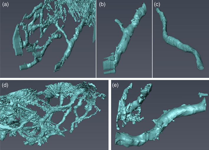
The 3D surface rendering of the lacunar–canaliculi network obtained from FIB‐SEM: (a–c) SEDC bone. (d,e) OI IV bone

2.3.3. TEM lamella sample preparation

The lamella preparation for TEM was performed in a dual‐beam FIB‐SEM (FEI Quanta FEG 600, Thermo Fisher Scientific), equipped with a gallium ion source operating in the accelerating voltage range 0.5–30 kV and an omniprobe micromanipulator. The same trimmed blocks that were used in the SSV procedure were employed in TEM lamella preparation as well. Using FIB milling, a lamella was cut parallel to the long axes of the mineralized collagen fibrils and analyzed by low dose electron tomography. Approximately 100‐nm thick sections from both bone samples were prepared for TEM studies using a FIB lift‐out technique (Figure 2).

FIGURE 2.

SEM images of some TEM lamella sample preparation steps. (a) Initially twisted plywood motif which is the region of interest was located. (b) Thin lamella from the region of interest was extracted and transferred to a TEM half grid. (c,d) Thinning and cleaning steps were performed to reach the desired sample thickness for electron tomography experiments. (e) Close‐up SEM image from the thin lamella. (f) TEM image of the prepared lamella

Regions of interest for TEM examination were identified by visualizing the surface of bone pieces by optical and scanning electron microscopy. A thin section was cut parallel to the orientation of the long axis of the bone implying that collagen fibrils are in‐plane view upon visualizing the thin section by TEM. Thin sections (10 μm × 10 μm × 0.1 μm) were transferred to a 3‐post lift‐out TEM half‐grid (Figure 3) (Agar Scientific AGJ420) for further electron tomography characterization.

FIGURE 3.

Mounting steps of 3‐post lift‐out TEM half‐grid containing extracted thin lamella from bone samples. (a) 3‐post lift‐out TEM half‐grid carefully inserted to the Autogrid, (b) Clip‐ring is placed to make sure that 3‐post lift‐out TEM half‐grid is stable enough to transfer inside the TEM, (c) zoomed‐in image of the part that thin lamella sits and (d) shows a representative image of thin lamella from bone samples

2.3.4. TEM tomography

Electron tomography was performed on the TU/e cryoTITAN (Thermo Fisher Scientific) operated at 300 kV, equipped with a field emission gun (FEG), a post‐column Gatan Energy Filter (GIF) and a post‐GIF 2 k × 2 k Gatan CCD camera. Electron tomography tilt series were taken by tilting the specimen from −65° to 65° with 2° per step. The alignment and 3D reconstruction of tilt series were done by using IMOD software using Simultaneous Iterative Reconstruction Technique (SIRT) with 20 iterations (Chen et al., 2014). Analysis of the reconstructed tilt series was done by using the software packages of Gatan Digital Micrograph, Avizo, and Image J.

Figure S16 shows an overview of the SEDC and OI type IV bone lamella. Most of the area shows clear banding patterns that are used to calculate the difference between the SEDC and OI type IV bone. The areas in the yellow boxes are some of the example regions where a clear D‐spacing is visible. The D‐spacing of the collagen periodical structure is determined by measuring over a distance containing at least 10 periods and calculating the average. Figures S17 and S18 show representative images. Moreover, to determine the orientation of the intrafibrillar crystals, an orientation analysis was performed. Tomographic slices were loaded as separate images to Matlab and the long and short axis of the crystals were manually set by clicking the four edges of the crystals. To avoid measuring the crystals twice, slices from the reconstruction that were at least 50 nm (in z‐direction) and 10 nm (in y‐direction) apart from each other were used.

2.4. Osteocyte lacunae and canaliculi

The nearest‐neighbor distances of the osteocytes were calculated by using images obtained by employing a POM (Appendix 6, Figure S10). After acquiring suitable images, the images were loaded into MATLAB and Image J, where the osteocytes were marked manually. Furthermore, the SEM/FIB SSV method allowed us to obtain a 3D reconstruction for the lacunar–canalicular network. The diameter of the canaliculi channels was measured using the individual images from which the reconstruction was made. The canaliculi (which are visible under POM as well, Figure S11) chosen to analyze were the ones that could be followed over the longest distance. These measurements were performed over the shortest and longest axis of the canaliculi to account for their irregular shape and with a spacing of 5 or 10 sequential images (Appendix 7, Figure S12).

2.5. Structural motifs

The 2D SEM imaging determined the periodicity of the twisted plywood motif while SEM FIB SSV provided us with 3D information regarding the specific collagen motifs within the bone samples to compare them with those shown in the literature before for human lamellar bone (Reznikov et al., 2014b). In OI type IV bone, due to the mutations, collagen fibrils form so‐called kinks in OI bone (Fratzl‐Zelman et al., 2014; Gjaltema & Bank, 2017) that might have an effect on the packing of the collagen on a larger scale and can lead to disruptions in the periodicity of the twisted plywood motif. For the analysis, 2D SEM imaging was done on areas that contain straight layers and occur near an osteon (Appendix 8, Figure S13). Scanning electron microscopy was used to determine the periodicity of the twisted plywood motif in both of cases. Imaging was focused primarily on what seemed to be straight layers that were near or in the circumference of an osteon. The reason why we picked those regions is to be consistent with both bone samples so that we would be able to determine the periodicity of the twisted plywood pattern more accurately. To have reliable and reproducible measurements regarding the periodicity of the twisted plywood motif, we moved radially outward from the central canal (where we observed vein) of the osteons at least one layer away, equivalent to about 3–5 μm (see Figure S13) Thereafter, the Plot Profile tool provided by Gatan Digital Micrograph and Image J was used to quantitatively measure the periodicity of the twisted plywood motif.

2.6. Characteristic features of collagen fibrils and minerals

Both POM and SEM (2D and FIB SSV) were used to evaluate differences between the structural motifs in SEDC and OI bone. For the POM observations, Picrosirius red staining of the collagen was used as described in the following reference (Eren et al., 2020). This staining is due to a strong binding interaction of the acidic sulfonic groups of the staining agent with the basic groups of the amino acids present in the collagen. The staining agent also permits birefringence analysis due to the parallel alignment of the dye molecules with the long axis of each collagen molecule, allowing the orientation of the collagen fibers to be determined (Kulkarni et al., 2014; Lattouf et al., 2014). The colors of the stained sections range from green to red under the polarizing microscope, which depends on the orientation and thickness of the section and the packing of the collagen fibers (Dayan, Hiss, Hirshberg, Bubis, & Wolman, 1989). Hence Picrosirius red staining was done to identify the orientation of collagen fibrils and/or fiber bundles in SEDC and OI bone (Appendix 9, Figure S14). Thereafter, TEM was used to evaluate the nanolevel differences between SEDC and OI type IV bone.

2.7. Effort‐time aspect of the presented approach

Table 1 summarizes the time required to obtain quantitative results starting from the native bone tissue to analyze the structural characteristics is shown. However, it needs to be noted that “required times” column (especially rows marked with asterisk) mentioned in the table is made by assuming one has enough knowledge and hands‐on experience in order to analyze the structural characteristics and handle the samples. Obviously, all the points mentioned in the table requires a learning curve meaning that in order to gain enough hands‐on experience a minimum of 3 months would have to be spent to be fluent.

TABLE 1.

A table demonstrating the required times to complete an experiment and/or analysis assuming the task is done by an experienced person, in particular for the tasks indicated by an asterisk

Experiment/analysis method	Required time (hours)
Fixation	~80
Demineralization	~80
Staining	~8
Embedding	~48
Cutting	~8
FIB/SSV	~16
ET	~16
ET‐3D reconstruction (IMOD)	~24*
FIB/SSV—3D reconstruction (Avizo)	~24*
Image analysis (MATLAB)	~24*
Image analysis (Image J)	~24*

3. RESULTS

3.1. Nearest‐neighbor distance of osteocytes

In SEDC bone osteocytes were present over the whole surface of an osteon (Figure 4a,b), while OI type IV bone always showed smaller island‐like structures that are spread over the surface and are either separated by the embedding material or biological material (Figure 4c,d). These island‐like structures were measured to be 65.6 ± 8.9 μm, where ± from now on indicates the sample standard deviation. As only one sample was used to evaluate the features, is not clear whether these island‐like structure should be attributed to the OI disease or not.

To quantitatively analyses the nearest‐neighbor distance of the osteocytes (Figure 5), a homemade MATLAB code was employed using POM images (Appendix 6, Figure S10). For SEDC bone, most of the distances fall in the 0–30 μm range being average distance 23 μm (Figure 5a). For the OI type IV bone, the average distance is longer (45 μm) and the most striking difference longer tailing up to 250 μm (Figure 5b). Fitting the distribution with a lognormal curve shows that both the mode and the standard deviation are larger for the OI type IV bone.

FIGURE 5.

The experimentally determined distribution of the nearest‐neighbor distances (histogram) and the fitted lognormal distribution (line) for (a) SEDC bone and (b) OI type IV bone

The average canaliculi diameter for SEDC bone was measured to be 547 ± 132 nm, while the average canaliculi diameter for OI Type IV was 413 ± 108 nm (Appendix 2, Table S3). The image collection was made by using the SSV procedure, for which we made sure that the cutting and subsequent imaging plane was perpendicular to the lacunar–canaliculi network, as shown clearly by the 3D reconstruction (Figure 6). A t‐test shows that the diameters of the OI bone are significantly different from that of the SEDC bone at the 5% significance level (Appendix S2).

Also the volume fractions of the lacunar‐canalicular network were measured (Figure S15), resulting in a volume fraction of 1.49 ± 0.45% for OI type bone compared with 0.75% ± 0.11% for SEDC bone (Appendix 10). Again, a t‐test shows that these values are significantly different at the 5% significance level (Appendix S2).

3.2. Structural motifs

In order to determine the periodicity of twisted plywood motif in SEDC and OI type IV bone samples, SEM was employed. The alteration of the direction of the collagen fibrils can be seen due to the contrast difference in the different orientations of the layers. The layers of the twisted plywood motif are clearly observed on the surface of the samples (Figure 7). Our results from SEDC bone indicate that the twisted plywood motif can be observed over almost the complete surface. The periodicity of the twisted plywood motif was determined (Figure 8), resulting in 4.9 ± 0.75 μm for SEDC bone and 3.2 ± 0.52 μm for OI type IV bone (Appendix 11, Table S4). A t‐test on the data indicates that the periodicity of the SEDC bone differs significantly from that of the OI Type IV bone at the 5% significance level (Appendix 2).

FIGURE 7.

Twisted plywood motifs for different bone types as obtained using 2D SEM: (a) SEDC bone and (b) OI type IV. Scale bars: 50 μm

Different types of structural motifs can be found in SEDC and OI type IV bone, in particular, aligned collagen fibrils coexist together with disordered collagen fibrils as demonstrated for healthy human lamellar bone (Reznikov et al., 2014b). (Figure 9, Supplementary Movie SM 1 and SM2). Although we tried to obtain the same quality for Figure 9c,d as for Figure 9a,b, this appeared to be experimentally impossible, the main reason being most likely a lower conductivity for the OI bone.

As explained and demonstrated for the first time by Reznikov et al. (2014b), human lamellar bone consists of ordered and disordered collagen motifs together with arrays of ordered collagen fibrils which were found to be 2–3 μm in diameter defined as “rods.” Here, in SEDC bone (Figure 9a,b) aligned collagen fibrils can be observed in two different orientations (marked with orange rectangle in Figure 9b), namely in‐plane and out‐of‐plane. In the SEDC bone aligned collagen fibrils form a bundle‐like structure with a thickness measured as 1.2–1.5 μm. All these arrays of aligned collagen fibrils are mainly within the lamellar plane that is also the imaging plane during the SSV procedure. Coexisting out‐of‐plane and in‐plane collagen fibrils are an inherent feature of human bone (Reznikov et al., 2014a). In the OI type IV bone sample (Figure 9c,d), similar as for SEDC bone, bundle‐like arrays of aligned collagen fibrils can be found. However, the thickness of bundle‐like collagen fibrils in the OI type IV bone was measured as 0.6–0.9 μm, which is significantly smaller than the about 1.5 μm obtained for SEDC bone (Figure 9b, the arrays of ordered collagen fibrils are marked with an orange rectangle). The aligned collagen fibrils are organized into several layers of parallel rods and the 3D analysis of OI type IV and SEDC bone show the presence of a rod‐like motif in both cases. In the SEDC bone, the diameter of the rod‐like motif is varying between 1.2 and 1.5 μm, which is not surprising as bone characteristics are affected by age (Wang, Shen, Li, & Mauli Agrawal, 2002) and possibly mutations. Next, bubble‐like small cavities throughout a given z‐thickness were measured (Figure 10, SM3 and SM4). In the OI samples the diameters of these bubble‐like cavities ranged between 80 and 100 nm and they span the whole z‐depth of the sample as used for the SSV procedure. Moreover, the volume fraction of these cavities was calculated and found to be 0.0274 ± 0.0021, where ± indicates the sample standard deviation (Appendix 10). While established methods were used for elucidating the structure (Boivin et al., 1990; Helfrich & Ralston, 2003; Keene & Tufa, 2010; Reznikov et al., 2013; Reznikov et al., 2018; Schwarcz, 2015; Seligman et al., 1966; Shah et al., 2019), for the SEDC bone these nanobubbles were completely absent, in spite of that more than 50 SSVs were collected in total for both type of samples.

FIGURE 10.

Images from 3D stacks of OI type IV bone: (a) slice #1, (b) slice #2, and (c) slice #3. The areas indicated by the yellow rectangle are shown enlarged in (d–f), respectively. One representative bubble‐like structure is marked with a white circle. This bubble‐like motif is first noticed in slice #1, reaches its maximum diameter in slice #2, 20 nm away, and disappears in slice #3, 60 nm further away

3.3. Characteristic features of collagen fibrils and minerals

To determine the nanolevel features of the SEDC and OI type IV bone samples, 100 nm thick sections from the cortical part of both bone pieces were prepared for further TEM characterization. The 2D projection images and images of these thin sections from SEDC and OI type IV bone are not strikingly different at first glance (Figure 11). Collagen fibrils and minerals predominantly lie in the imaging plane of thin sections and therefore minerals and the characteristic D‐spacing of collagen fibrils can be observed.

In Figure 11, both in the SEDC and OI type IV bone images, black dots that are spanning the whole section, are gold nanoparticles which were used as fiducial markers for the 3D reconstruction. In OI type IV and SEDC bone, collagen fibrils are identifiable in 2D TEM images by the presence of the gap and overlap regions that are repeated along the lengths of the thin slices (Figure 11a,b). The average D‐spacing values for SEDC bone was 66.8 ± 0.8 nm, while for the OI type IV it was 62.0 ± 0.6 nm (Appendix 12, Figures S16–S18). 2D TEM images allow us to determine that the gap/overlap regions extend in almost perfect registry between adjacent collagen fibrils as shown in the literature (McNally et al., 2012). Moreover, as for the collagen fibrils, the mineral particles (indicated with yellow arrows in Figure 11c–f) also show similar characteristics in terms of orientation relative to c‐axis of collagen fibrils and appearance, in OI type IV and SEDC bone (Figure 11c–f).

Although 2D projection images are not strikingly different, nanolevel structures of SEDC (Figure 12, SM5) and OI type IV bone (Figure 13, SM6) show clear differences after 3D reconstruction of the electron tomography data (Figures 12 and 13). Using FIB milling, a 100 nm thick lamella was cut from each sample parallel to the long axes of the mineralized collagen fibrils and analyzed by low dose electron tomography. To optimize contrast for visual purpose only, 100 z‐slices (slice thickness 0.75 nm) of the tomographic reconstruction were averaged (Figure 12a) to generate a 2D projected volume with a thickness of 75 nm. The resulting 2D projection showed a collagen fibril with a diameter of approximately 100 nm (Figure 12b), displaying again the characteristic approximately 67 nm banding pattern for the SEDC sample and approximately 62 nm for the OI type IV bone sample. Analysis of the orientation of the intrafibrillar crystals confirmed that they were aligned along the long axis of the collagen fibril, with an angular distribution having a half‐width of about 15° (Figure 12g, Appendix 13, Figures S19 and S20) for SEDC bone. Additionally, orientation analysis was conducted by viewing the tomographic reconstruction along the collagen fibril axis (Figure 12c–f). The 2D projections of 10 added adjacent tomographic xz slices (total slice thickness 7.5 nm) showed that intrafibrillar crystals were randomly oriented in lateral directions, consistent with recent results (Xu et al., 2020) and have no preferred lateral orientation, with an angular distribution having a half‐width of about 60° (Figure 12h) for SEDC bone.

The first noticeable difference between the OI type IV and the SEDC bone is the disturbed packing of collagen fibrils. In SEDC bone, there is little or no space between the collagen fibrils. However, in OI type IV bone, the space between the collagen fibrils is increased, resulting in hollow zones containing neither crystals nor collagen fibrils (Figure 13a,b). The orientation of the crystals shows differences as well. While for the SEDC bone orientation analysis of the intrafibrillar crystals from the tomogram confirmed a longitudinal angular distribution with a half‐width at half maximum of about 16°, (Figure 12g; Figure S20a), for OI type IV bone a similar orientation analysis showed a half‐width half maximum of about 34° (Figure 13g; Figure S20b). Additionally, orientation analysis was conducted by viewing the tomographic reconstruction along the collagen fibril axis (Figures 12 and 13c–f). The 2D projections of 10 added adjacent tomographic xz slices (total slice thickness 7.5 nm) showed that the intrafibrillar crystals were again randomly oriented in the lateral direction and have no preferred lateral orientation, with an angular distribution having a half‐width of about 60°, similar to the SEDC bone sample.

A more detailed analysis of a single collagen fibril from OI type IV bone is shown in Figure 14. This mineralized single collagen fibril viewed from the top (Figure 14a–d; SM7) and along the fibril (Figure 14e,f; SM8) shows disturbed regions in the hierarchy of mineralized collagen fibril structure. Several stacks of crystals can be seen in Figure 14c (marked with a red rectangle), which are tightly packed together and oriented with their c‐axis along the fibril. The region just below that shows a clear gap between the crystals. The same defect can be followed from Figure 14b–d, proving that it spans the whole collagen fibril (SM7 and SM8). The cross‐sections of regions highlighted in Figure 14c show stacks of crystals (marked with a white circle) (Figure 14e) and defected area between crystals (marked with a yellow square) (Figure 14f).

Moreover, a single mineralized collagen fibril from SEDC bone was analyzed as well. This fibril viewed from the top (Figure 15a–d) and along the fibril (Figure 15e,f) demonstrates that defects as found in OI type IV bone were less prominently present in the structure of this single collagen fibril in the SEDC bone. Stacks of intrafibrillar crystals can be seen in the top views (marked with red rectangles) and cross‐sectional views (marked with white circles). It is clear from the top views that tightly packed intrafibrillar crystals are oriented with their c‐axis along the fibril. The cross‐sectional views of regions highlighted in top views similarly show stacks of crystals.

4. DISCUSSION

We have chosen to perform the analyses on only two pathological bone specimens: one from the tibia of a 6‐year‐old patient with spondyloepiphyseal dysplasia congenital (SEDC) and one from the femur of an 8‐year‐old OI type IV patient. We have no indications that the age difference between the two patients or the site difference (femur vs. tibia) attributes to the anomalies that we have found. However, our findings can certainly not be generalized to all OI bone, not even to OI type IV, nor to SEDC bones. It should be realized that the classification of OI is based on clinical severity and not on the genetic mutation concerned. There is a plethora of genetic mutations in collagen type I that can lead to the various clinical subtypes and even the same genetic mutation within two family members can lead to different disease severities. Moreover, it is crucial to mention that as far as the authors are aware, there are no articles published on the structural analysis of bone with SEDC disease. Our current findings provide comprehensive data on potential (or new) tissue anomalies in OI bone but requires much more additional research that may copy our methodology and subsequently make a connection to bone stiffness and strength, and its subsequent disease severity.

It is important to note that, when analyzing bone samples by using polarized light microscopy, birefringence is thought to be an indication regarding the orientation of collagen fibers as collagen is an anisotropic material. When the collagen fibers are parallel to the light source, they appear darker and when the collagen fibers are perpendicular to the light source, they appear brighter (Bromage et al., 2003; Dede Eren et al., 2021) which helps identify the orientation of collagen fibers. However, one should be careful while relying on only polarized light microscope when determining the orientation of collagen fibers due to an effect called differential birefringence which is based on the thickness of the section (Bromage et al., 2003) taken from bone samples and it is crucial to be consistent in terms of the thickness of the sample during sample preparation. Moreover, as shown in this study by using OTOTO staining, we were able to image osteocytes and their dendritic extensions by using POM.

However, POM alone is not enough to determine the ultrastructure of neither for pathological bone, nor for healthy bone. To obtain complementary data, one can employ SEM and FIB‐SSV which allows thin layers to be serially milled away by using an ion beam, thereby exposing a fresh layer. Thereafter, each layer is subsequently scanned by electron beam, and this process eventually provides a detailed 3D image. In the past, several authors demonstrated that by using this particular method, it is possible to demonstrate organization of collagen fibers (Faingold, Cohen, Reznikov, & Wagner, 2013; Reznikov et al., 2014b). By using SSV method, Reznikov et al. showed that rat bone has organized and disorganized layers of collagen fibrils, while in human bone there is extra level of complexity, which was defined as rods consisting of arrays of ordered collagen fibrils. Here, for the first time we showed that same techniques can be employed by using two different pathological bone tissues.

Moreover, the layer thickness has been measured by several researchers by using various methods with mixed and inconsistent results. For example, it has been reported that the layers of human collagen fibrils have a periodicity of 5–7 μm (Wagermaier et al., 2006), 6–9 μm (Reznikov et al., 2014b), 9.06 ± 2.13 μm (Pazzaglia, Congiu, Marchese, Spagnuolo, & Quacci, 2012), or 4–8 μm (Varga et al., 2013), corresponding to a single layer. These discrepancies can be related with the methods that have been used to measure the thickness of a layer, the bone tissue used, number of measurements made as well as the age and gender of the individuals that have been used for the studies. Here we found that the layer thickness for SEDC bone was measured as 4.9 ± 0.75 μm and 3.2 ± 0.52 μm for OI type IV bone.

Importantly, as bone has a complex hierarchical organization spanning across multiple levels, FIB equipped scanning electron microscopy can do more than serial slice and view. By using FIB‐SEM, TEM lamella preparation, where the sample thickness must be approximately 100 nm in order to achieve optimum electron transparency, is possible. After preparing the thin lamella with a desired thickness, electron tomography can be used to determine the nanolevel features of pathological or healthy bone tissue. Previously, it has been showed that ultrastructural organization of collagen fibrils and crystal in healthy bone can be investigated by using electron tomography (Reznikov et al., 2018). Here, we demonstrated that by using techniques such as thin lamella preparation and electron tomography, pathological tissue can be analyzed, and the nanolevel organization of this tissue obtained, which might shed light on pathological mineralization of these tissues.

Summarizing, the 3D organization of bone tissue, whether healthy or pathological, is an important issue. By having only 2D images, it is extremely hard, if not impossible, to assess and determine the true nature of integral parts of bone tissue. Methods, such as FIB‐SSV and ET, are rather useful in determining the 3D organization of bone tissues and we tried to explore part of a terra incognita by employing these imaging techniques to two pathological bone tissues. It should be noted that such an analysis requires substantial effort, and, at present, this limits the number of samples. By using a large number of samples employing the methods described in this article, a unifying picture regarding both types of pathological bone tissue can be potentially drawn.

5. CONCLUSIONS

In this article, we showed the possibilities of employing different microscopy techniques to characterize bone tissue. While the differences that we have found for the pathological tissues cannot be generalized, neither for OI Type IV, nor for SEDC bone, it is clear that the microscopy methods are useful and crucial in understanding the multiscale hierarchical organization of (pathological) bone tissue. By using the techniques reported in this article, one can determine quantitative results regarding the nearest‐neighbor distances of osteocytes, average canaliculi diameter, canalicular density, the periodicity of the twisted plywood motif, the microlevel and nanolevel hierarchy of collagen fibers and fibrils, and the inherent characteristics of mineral particles in a given bone tissue.

It is also important to mention that while this article employed pathological bone tissues, electron microscopy techniques, such as FIB‐SSV and ET, can be used in any mineralized or non‐mineralized tissue. Both electron and light microscopy techniques are based on 2D observations or projections of 3D complex structures and due to the multiscale hierarchical organization of bone tissues, conventional 2D techniques are sometimes hard to interpret. It is important to note that, while 2D imaging techniques can provide an initial understanding regarding the pathological or healthy bone tissues, due to the complex structural hierarchy of these tissues, 3D imaging techniques are able to reveal differences in structural details that otherwise might go unnoticed. To fully determine and understand the hierarchical structure and possible structural alterations of pathological bone is even more challenging. Approaches combining conventional and advanced techniques, which provide consistent and reliable results, is a must and can pave the way for better understanding the organization of healthy bone and disturbed organization of pathological bone and finally find cues to repair these disorders. As a thorough knowledge of the structures of pathological bone tissues is the key to understand the changes occurring during diseases, such knowledge also will be helpful to determine the underlying mechanisms that are responsible for pathologies. Therefore, 3D imaging techniques, in particular FIB/SSV and electron tomography, can play a significant role to reshape our understanding of healthy and pathological tissues.

CONFLICT OF INTEREST

The authors declare no conflicts of interest.

AUTHOR CONTRIBUTIONS

This article contains contributions from authors active in various disciplines. E. Deniz Eren: Did larger part of the analysis work; conceived the article and discussed with all other authors. Wouter H. Nijhuis: Surgical part and clinical background. Freek van der Weel: Contributed to analysis work. Aysegul Dede Eren: Contributed to analysis work. Sana Ansari: Contributed to analysis work. Paul H.H. Bomans: Contributed to analysis work. Heiner Friedrich: Contributed to analysis work. Ralph J. Sakkers: Surgical part and clinical background. Harrie Weinans: Surgical part and clinical background. Gijsbertus de With: Contributed to analysis work; conceived the article and discussed with all other authors.

Supporting information

Appendices 1‐14: Supporting Information.

Movie S1 Stack of images from SSV procedure showing different types of motifs in control bone.

Movie S2 Stack of images from SSV procedure showing different types of motifs in OI Type IV bone.

Movie S3 Stack of images from SSV procedure showing bubble‐like small cavities found in OI Type IV bone from the embedded sample.

Movie S4 Stack of images from SSV procedure showing bubble‐like small cavities found in OI Type IV bone in the air‐dried sample.

Movie S5 Electron tomographic reconstruction slices viewed from the top of the SEDC bone lamella, showing an overview of the sample.

Movie S6 Electron tomographic reconstruction slices viewed from the top of the OI Type IV bone lamella, showing an overview of the sample.

Movie S7 Electron tomographic reconstruction slices viewed from the top of the single collagen fibril in OI Type IV bone.

Movie S8 Electron tomographic reconstruction slices viewed along the single collagen fibril in OI Type IV bone.

Eren, E. D. , Nijhuis, W. H. , van der Weel, F. , Dede Eren, A. , Ansari, S. , Bomans, P. H. H. , Friedrich, H. , Sakkers, R. J. , Weinans, H. , & de With, G. (2022). Multiscale characterization of pathological bone tissue. Microscopy Research and Technique, 85(2), 469–486. 10.1002/jemt.23920

DATA AVAILABILITY STATEMENT

The data that support the findings of this study are available from the corresponding author upon reasonable request.

REFERENCES

- Bakker, A. D. , & Klein‐Nulend, J. (2012). Osteoblast isolation from murine calvaria and long bones. In Helfrich M. H. & Ralston S. (Eds.), Bone research protocols (Vol. 2019, pp. 19–29). New York, NY: Humana Press. [DOI] [PubMed] [Google Scholar]
- Bishop, N. (2016). Bone material properties in osteogenesis imperfecta. Journal of Bone and Mineral Research, 31, 699–708. [DOI] [PubMed] [Google Scholar]
- Boivin, G. , Anthoine‐Terrier, C. , & Obrant, K. J. (1990). Transmission electron microscopy of bone tissue: A review. Acta Orthopaedica, 61, 170–180. [DOI] [PubMed] [Google Scholar]
- Boskey, A. L. , & Imbert, L. (2017). Bone quality changes associated with aging and disease: A review. Ann N Y Acad Sci, 1410(1), 93–106. [DOI] [PMC free article] [PubMed] [Google Scholar]
- Boskey, A. L. , & Robey, P. G. (2018). The composition of bone. In Bilezikian J. P. (Ed.), Primer on the metabolic bone diseases and disorders of mineral metabolism (pp. 84–92). Hoboken, USA: Wiley‐Blackwell. 10.1002/9781119266594.ch11 [DOI] [Google Scholar]
- Boyde, A. , & Riggs, C. M. (1990). The quantitative study of the orientation of collagen in compact bone slices. Bone, 11, 35–39. [DOI] [PubMed] [Google Scholar]
- Bromage, T. G. , Goldman, H. M. , SC, M. F. , Warshaw, J. , Boyde, A. , & Riggs, C. M. (2003). Circularly polarized light standards for investigations of collagen fiber orientation in bone. Anatomical Record. Part B, New Anatomist, 274, 157–168. [DOI] [PubMed] [Google Scholar]
- Cassella, J. P. , Barber, P. , Catterall, A. C. , & Ali, S. Y. (1994). A morphometric analysis of osteoid collagen fibril diameter in osteogenesis imperfecta. Bone, 15, 329–334. [DOI] [PubMed] [Google Scholar]
- Central Committee on Research Involving Human Subjects . (2021). https://english.ccmo.nl/investigators/legal-framework-for-medical-scientific-research/your-research-is-it-subject-to-the-wmo-or-not
- Chen, D. , Goris, B. , Bleichrodt, F. , Mezerji, H. H. , Bals, S. , Batenburg, K. J. , … Friedrich, H. (2014). The properties of SIRT, TVM, and DART for 3D imaging of tubular domains in nanocomposite thin‐films and sections. Ultramicroscopy, 147, 137–148. [DOI] [PubMed] [Google Scholar]
- Cressey, B. A. , & Cressey, G. (2003). A model for the composite nanostructure of bone suggested by high‐resolution transmission electron microscopy. Mineralogical Magazine, 67, 1171–1182. [Google Scholar]
- Dayan, D. , Hiss, Y. , Hirshberg, A. , Bubis, J. J. , & Wolman, M. (1989). Are the polarization colors of Picrosirius red‐stained collagen determined only by the diameter of the fibers? Histochemistry, 93, 27–29. [DOI] [PubMed] [Google Scholar]
- Dede Eren, A. , Vasilevich, A. , Eren, E. D. , Sudarsanam, P. , Tuvshindorj, U. , de Boer, J. , & Foolen, J. (2020). Tendon‐derived biomimetic surface topographies induce phenotypic maintenance of tenocytes in vitro. Tissue Engineering Part A, 00, 1–14. [DOI] [PubMed] [Google Scholar]
- Dede Eren, A. , Eren, E. D. , TJS, W. , de Boer, J. , Gelderblom, H. , & Foolen, J. (2021). Self‐agglomerated collagen patterns govern cell behaviour. Scientific Reports, 11, 1–14. [DOI] [PMC free article] [PubMed] [Google Scholar]
- Deshpande, A. S. , & Beniash, E. (2008). Bioinspired synthesis of mineralized collagen fibrils. Crystal Growth & Design, 8, 3084–3090. [DOI] [PMC free article] [PubMed] [Google Scholar]
- Eimar, H. , Tamimi, F. , Retrouvey, J. M. , Rauch, F. , Aubin, J. E. , & McKee, M. D. (2016). Craniofacial and dental defects in the Col1a1 Jrt/+ mouse model of osteogenesis imperfecta. Journal of Dental Research, 95, 761–768. [DOI] [PubMed] [Google Scholar]
- Eppell, S. J. , Tong, W. , Lawrence Katz, J. , Kuhn, L. , & Glimcher, M. J. (2001). Shape and size of isolated bone mineralites measured using atomic force microscopy. Journal of Orthopaedic Research, 19, 1027–1034. [DOI] [PubMed] [Google Scholar]
- Eren, A. D. , Sinha, R. , Eren, E. D. , Yuan, H. , İz, S. , Valster, H. , … Boer, J. (2020). Decellularized porcine Achilles tendon induces anti‐inflammatory macrophage phenotype in vitro and tendon repair in vivo. Journal of Immunology and Regenerative Medicine, 8, 100027. [Google Scholar]
- Erickson, B. , Fang, M. , Wallace, J. M. , Orr, B. G. , Les, C. M. , & Banaszak Holl, M. M. (2013). Nanoscale structure of type I collagen fibrils: Quantitative measurement of D‐spacing. Biotechnology Journal, 8, 117–126. [DOI] [PMC free article] [PubMed] [Google Scholar]
- Faingold, A. , Cohen, S. R. , Reznikov, N. , & Wagner, H. D. (2013). Osteonal lamellae elementary units: Lamellar microstructure, curvature and mechanical properties. Acta Biomaterialia, 9, 5956–5962. [DOI] [PubMed] [Google Scholar]
- Fratzl‐Zelman, N. , Schmidt, I. , Roschger, P. , Glorieux, F. H. , Klaushofer, K. , Fratzl, P. , … Wagermaier, W. (2014). Mineral particle size in children with osteogenesis imperfecta type I is not increased independently of specific collagen mutations. Bone, 60, 122–1128. [DOI] [PubMed] [Google Scholar]
- Gebhardt, W. (1905). Über funktionell wichtige anordnungsweisen der feineren und gröberen bauelemente des wirbeltierknochens. Archiv für Entwicklungsmechanik der Organismen, 20, 187–322. [Google Scholar]
- Georgiadis, M. , Müller, R. , & Schneider, P. (2016). Techniques to assess bone ultrastructure organization: Orientation and arrangement of mineralized collagen fibrils. Journal of the Royal Society Interface, 13, 20160088. [DOI] [PMC free article] [PubMed] [Google Scholar]
- Gjaltema, R. A. F. , & Bank, R. A. (2017). Molecular insights into prolyl and lysyl hydroxylation of fibrillar collagens in health and disease. Critical Reviews in Biochemistry and Molecular Biology, 52, 74–95. [DOI] [PubMed] [Google Scholar]
- Grandfield, K. , Vuong, V. , & Schwarcz, H. P. (2018). Ultrastructure of bone: Hierarchical features from nanometer to micrometer scale revealed in focused ion beam sections in the TEM. Calcified Tissue International, 103, 606–616. [DOI] [PubMed] [Google Scholar]
- Habelitz, S. , Balooch, M. , Marshall, S. J. , Balooch, G. , & Marshall, G. W. (2002). In situ atomic force microscopy of partially demineralized human dentin collagen fibrils. Journal of Structural Biology, 138, 227–236. [DOI] [PubMed] [Google Scholar]
- Hassenkam, T. , Fantner, G. E. , Cutroni, J. A. , Weaver, J. C. , Morse, D. E. , & Hansma, P. K. (2004). High‐resolution AFM imaging of intact and fractured trabecular bone. Bone, 35, 4–10. [DOI] [PubMed] [Google Scholar]
- Helfrich, M. , & Ralston, S. (2003). Bone reseacrh protocols (Vol. 80). Totowa, New Jersey: Humana Press. [Google Scholar]
- Keene, D. R. , & Tufa, S. F. (2010). Transmission electron microscopy of cartilage and bone. Methods in Cell Biology, 96, 443–473. [DOI] [PubMed] [Google Scholar]
- Kivirikko, K. I. (1993). Collagens and their abnormalities in a wide spectrum of diseases. Annals of Medicine, 25, 113–126. [DOI] [PubMed] [Google Scholar]
- Kłosowski, M. M. , Carzaniga, R. , Abellan, P. , Ramasse, Q. , McComb, D. W. , Porter, A. E. , & Shefelbine, S. J. (2017). Electron microscopy reveals structural and chemical changes at the nanometer scale in the osteogenesis imperfecta murine pathology. ACS Biomaterials Science & Engineering, 3, 2788–2797. [DOI] [PubMed] [Google Scholar]
- Kulkarni, R. R. , Sarvade, S. D. , Boaz, K. , Srikant, N. , Kp, N. , & Lewis, A. J. (2014). Polarizing and light microscopic analysis of mineralized components and stromal elements in fibrous ossifying lesions. Journal of Clinical and Diagnostic Research, 8, 42–45. [DOI] [PMC free article] [PubMed] [Google Scholar]
- Lattouf, R. , Younes, R. , Lutomski, D. , Naaman, N. , Godeau, G. , Senni, K. , & Changotade, S. (2014). Picrosirius red staining: A useful tool to appraise collagen networks in normal and pathological tissues. The Journal of Histochemistry and Cytochemistry, 62, 751–758. [DOI] [PubMed] [Google Scholar]
- Lefèvre, E. , Guivier‐Curien, C. , Pithioux, M. , & Charrier, A. (2013). Determination of mechanical properties of cortical bone using AFM under dry and immersed conditions. Computer Methods in Biomechanics and Biomedical Engineering, 16, 337–339. [DOI] [PubMed] [Google Scholar]
- Li, T. , Chang, S.‐W. , Florez, N. R. , Buehler, M. J. , Shefelbine, S. , Dao, M. , & Zeng, K. (2016). Studies of chain substitution caused sub‐fibril level differences in stiffness and ultrastructure of wildtype and oim/oim collagen fibers using multifrequency‐AFM and molecular modeling. Biomaterials, 107, 15–22. [DOI] [PMC free article] [PubMed] [Google Scholar]
- Linder, L. , Albrektsson, T. , Branemark, P. I. , Hansson, H. A. , Ivarsson, B. , Jonsson, U. , & Lundström, I. (1983). Electron microscopic analysis of the bone‐titanium interface. Acta Orthopaedica, 54, 45–52. [DOI] [PubMed] [Google Scholar]
- Marini, J. C. , Forlino, A. , Cabral, W. A. , Barnes, A. M. , San Antonio, J. D. , Milgrom, S. , … Byers, P. H. (2007). Consortium for osteogenesis imperfecta mutations in the helical domain of type I collagen: Regions rich in lethal mutations align with collagen binding sites for integrins and proteoglycans. Human Mutation, 28, 209–221. [DOI] [PMC free article] [PubMed] [Google Scholar]
- Marini, J. C. , Forlino, A. , Bächinger, H. P. , Bishop, N. J. , Byers, P. H. , Paepe, A. , … Semler, O. (2017). Osteogenesis imperfecta. Nature Reviews Disease Primers, 3, 1–19. [DOI] [PubMed] [Google Scholar]
- McNally, E. , Nan, F. , Botton, G. A. , & Schwarcz, H. P. (2013). Scanning transmission electron microscopic tomography of cortical bone using Z‐contrast imaging. Micron, 49, 46–53. [DOI] [PubMed] [Google Scholar]
- McNally, E. A. , Schwarcz, H. P. , Botton, G. A. , & Arsenault, A. L. (2012). A model for the ultrastructure of bone based on electron microscopy of ion‐milled sections. PLoS One, 7, 1–12. [DOI] [PMC free article] [PubMed] [Google Scholar]
- Mendonça, G. , Mendonça, D. B. S. , Aragão, F. J. L. , & Cooper, L. F. (2008). Advancing dental implant surface technology: From micron‐ to nanotopography. Biomaterials, 29, 3822–3835. [DOI] [PubMed] [Google Scholar]
- Mitchell, J. , & Van Heteren, A. H. (2016). A literature review of the spatial organization of lamellar bone. Comptes Rendus Palevol, 15, 23–31. [Google Scholar]
- Mohammadi, P. , Aranko, A. S. , Landowski, C. P. , Ikkala, O. , Jaudzems, K. , Wagermaier, W. , & Linder, M. B. (2019). Biomimetic composites with enhanced toughening using silk‐inspired triblock proteins and aligned nanocellulose reinforcements. Science Advances, 5, eaaw2541. 10.1126/sciadv.aaw2541 [DOI] [PMC free article] [PubMed] [Google Scholar]
- Nijhuis, W. H. , Eastwood, D. M. , Allgrove, J. , Hvid, I. , Weinans, H. H. , Bank, R. A. , & Sakkers, R. J. (2019). Current concepts in osteogenesis imperfecta: Bone structure, biomechanics and medical management. Journal of Children's Orthopaedics, 13, 1–11. [DOI] [PMC free article] [PubMed] [Google Scholar]
- Pazzaglia, U. E. , Congiu, T. , Marchese, M. , Spagnuolo, F. , & Quacci, D. (2012). Morphometry and patterns of lamellar bone in human Haversian systems. The Anatomical Record, 295, 1421–1429. [DOI] [PubMed] [Google Scholar]
- Prockop, D. J. (1990). Minireview mutations that alter the primary structure of type I collagen. Biochemistry, 265, 15349–15352. [PubMed] [Google Scholar]
- Reznikov, N. , Almany‐Magal, R. , Shahar, R. , & Weiner, S. (2013). Three‐dimensional imaging of collagen fibril organization in rat circumferential lamellar bone using a dual beam electron microscope reveals ordered and disordered sub‐lamellar structures. Bone, 52, 676–683. [DOI] [PubMed] [Google Scholar]
- Reznikov, N. , Bilton, M. , Lari, L. , Stevens, M. M. , & Kröger, R. (2018). Fractal‐like hierarchical organization of bone begins at the nanoscale. Science, 360, eaao2189. [DOI] [PMC free article] [PubMed] [Google Scholar]
- Reznikov, N. , Shahar, R. , & Weiner, S. (2014a). Bone hierarchical structure in three dimensions. Acta Biomaterialia, 10, 3815–3826. [DOI] [PubMed] [Google Scholar]
- Reznikov, N. , Shahar, R. , & Weiner, S. (2014b). Three‐dimensional structure of human lamellar bone: The presence of two different materials and new insights into the hierarchical organization. Bone, 59, 93–104. [DOI] [PubMed] [Google Scholar]
- Rieppo, J. , Hallikainen, J. , Jurvelin, J. S. , Kiviranta, I. , Helminen, H. J. , & Hyttinen, M. M. (2008). Practical considerations in the use of polarized light microscopy in the analysis of the collagen network in articular cartilage. Microscopy Research and Technique, 71, 279–287. [DOI] [PubMed] [Google Scholar]
- Rivera, J. , Hosseini, M. S. , Restrepo, D. , Murata, S. , Vasile, D. , Parkinson, D. Y. , … Kisailus, D. (2020). Toughening mechanisms of the elytra of the diabolical ironclad beetle. Nature, 586, 543–548. [DOI] [PubMed] [Google Scholar]
- Rubin, M. A. , Jasiuk, I. , Taylor, J. , Rubin, J. , Ganey, T. , & Apkarian, R. P. (2003). TEM analysis of the nanostructure of normal and osteoporotic human trabecular bone. Bone, 33, 270–282. [DOI] [PubMed] [Google Scholar]
- Sarathchandra, P. , Pope, F. M. , & Ali, S. Y. (1999). Morphometric analysis of type I collagen fibrils in the osteoid of osteogenesis imperfecta. Calcified Tissue International, 65, 390–395. [DOI] [PubMed] [Google Scholar]
- Schrof, S. , Varga, P. , Galvis, L. , Raum, K. , & Masic, A. (2014). 3D Raman mapping of the collagen fibril orientation in human osteonal lamellae. Journal of Structural Biology, 187, 266–275. [DOI] [PubMed] [Google Scholar]
- Schwarcz, H. P. (2015). The ultrastructure of bone as revealed in electron microscopy of ion‐milled sections. Seminars in Cell & Developmental Biology, 46, 44–50. [DOI] [PubMed] [Google Scholar]
- Seligman, A. M. , Wasserkrug, H. L. , & Hanker, J. S. (1966). A new staining method (OTO) for enhancing contrast of lipid—containing membranes and droplets in osmium tetroxide—fixed tissue with osmiophilic thiocarbohydrazide(TCH). The Journal of Cell Biology, 30, 424–432. [DOI] [PMC free article] [PubMed] [Google Scholar]
- Shah, F. A. , Ruscsák, K. , & Palmquist, A. (2019). 50 years of scanning electron microscopy of bone—A comprehensive overview of the important discoveries made and insights gained into bone material properties in health, disease, and taphonomy. Bone Research, 7, 1–15. [DOI] [PMC free article] [PubMed] [Google Scholar]
- Shahar, R. , & Weiner, S. (2018). Open questions on the 3D structures of collagen containing vertebrate mineralized tissues: A perspective. Journal of Structural Biology, 201, 187–198. [DOI] [PubMed] [Google Scholar]
- Soleimani, M. , Rutten, L. , Maddala, S. P. , Wu, H. , Eren, E. D. , Mezari, B. , … RATM, V. B. (2020). Modifying the thickness, pore size, and composition of diatom frustule in Pinnularia sp. with Al3+ ions. Scientific Reports, 10, 1–12. [DOI] [PMC free article] [PubMed] [Google Scholar]
- Su, X. , Sun, K. , Cui, F. Z. , & Landis, W. J. (2003). Organization of apatite crystals in human woven bone. Bone, 32, 150–162. [DOI] [PubMed] [Google Scholar]
- Sun, J. , & Bhushan, B. (2012). Hierarchical structure and mechanical properties of nacre: A review. RSC Advances, 2, 7617–7632. [Google Scholar]
- Thomson, J. W. (1927). Osteogenesis imperfecta. Lancet, 209, 103. [Google Scholar]
- Thorfve, A. , Palmquist, A. , & Grandfield, K. (2015). Three‐dimensional analytical techniques for evaluation of osseointegrated titanium implants. Materials Science and Technology, 31, 174–179. [Google Scholar]
- Tong, W. , Glimcher, M. J. , Katz, J. L. , Kuhn, L. , & Eppell, S. J. (2003). Size and shape of mineralites in young bovine bone measured by atomic force microscopy. Calcified Tissue International, 72, 592–598. [DOI] [PubMed] [Google Scholar]
- Van Dijk, F. S. , & Sillence, D. O. (2014). Osteogenesis imperfecta: Clinical diagnosis, nomenclature and severity assessment. American Journal of Medical Genetics‐Part A, 164, 1470–1481. [DOI] [PMC free article] [PubMed] [Google Scholar]
- Van Dijk, F. S. , Cobben, J. M. , Kariminejad, A. , Maugeri, A. , Nikkels, P. G. , Van Rijn, R. R. , & Pals, G. (2011). Osteogenesis imperfecta: A review with clinical examples. Molecular Syndromology, 2, 1–20. [DOI] [PMC free article] [PubMed] [Google Scholar]
- Varga, P. , Pacureanu, A. , Langer, M. , Suhonen, H. , Hesse, B. , Grimal, Q. , … Peyrin, F. (2013). Investigation of the three‐dimensional orientation of mineralized collagen fibrils in human lamellar bone using synchrotron X‐ray phase nano‐tomography. Acta Biomaterialia, 9, 8118–8127. [DOI] [PubMed] [Google Scholar]
- Wagermaier, W. S. , Gupta, H. , Gourrier, A. , Burghammer, M. , Roschger, P. , & Fratzl, P. (2006). Spiral twisting of fiber orientation inside bone lamellae. Biointerphases, 1, 1–5. [DOI] [PubMed] [Google Scholar]
- Wallace, J. M. (2012). Applications of atomic force microscopy for the assessment of nanoscale morphological and mechanical properties of bone. Bone, 50, 420–427. [DOI] [PubMed] [Google Scholar]
- Wang, X. , Shen, X. , Li, X. , & Mauli Agrawal, C. (2002). Age‐related changes in the collagen network and toughness of bone. Bone, 31, 1–7. [DOI] [PubMed] [Google Scholar]
- Wegst, U. G. K. , Bai, H. , Saiz, E. , Tomsia, A. P. , & Ritchie, R. O. (2015). Bioinspired structural materials. Nature Materials, 14, 23–36. [DOI] [PubMed] [Google Scholar]
- Weiner, S. , & Traub, W. (1989). Crystal size and organization in bone. Connective Tissue Research, 21, 259–265. [DOI] [PubMed] [Google Scholar]
- Weiner, S. , Traub, W. , & Wagner, H. D. (1999). Lamellar bone: Structure‐function relations. Journal of Structural Biology, 126, 241–255. [DOI] [PubMed] [Google Scholar]
- Weiner, S. , & Wagner, H. D. (1998). The material bone: Structure‐mechanical function relations. Annual Review of Materials Science, 28, 271–298. [Google Scholar]
- Weiner, S. , Arad, T. , & Traub, W. (1991). Crystal organization in rat bone lamellae. FEBS Letters, 285, 49–54. [DOI] [PubMed] [Google Scholar]
- Wolman, M. , & Kasten, F. H. (1986). Polarized light microscopy in the study of the molecular structure of collagen and reticulin. Histochemistry, 85, 41–49. [DOI] [PubMed] [Google Scholar]
- Xu, Y. F. , Nudelman, F. , Eren, E. D. , Wirix, M. J. M. , Cantaert, B. , Nijhuis, W. H. , … Sommerdijk, N. (2020). Intermolecular channels direct crystal orientation in mineralized collagen. Nature Communications, 11, 1–12. [DOI] [PMC free article] [PubMed] [Google Scholar]
- Yao, H. , Dao, M. , Imholt, T. , Huang, J. , Wheeler, K. , Bonilla, A. , … Ortiz, C. (2010). Proceedings of the National Academy of Sciences of the Unites States of America. Protection mechanisms of the iron‐plated armor of a deep‐sea hydrothermal vent gastropod, 107, 987–992. [DOI] [PMC free article] [PubMed] [Google Scholar]
Associated Data
This section collects any data citations, data availability statements, or supplementary materials included in this article.
Supplementary Materials