Resolving the SLOSS dilemma for biodiversity conservation: a research agenda

ABSTRACT

The legacy of the ‘SL > SS principle’, that a single or a few large habitat patches (SL) conserve more species than several small patches (SS), is evident in decisions to protect large patches while down‐weighting small ones. However, empirical support for this principle is lacking, and most studies find either no difference or the opposite pattern (SS > SL). To resolve this dilemma, we propose a research agenda by asking, ‘are there consistent, empirically demonstrated conditions leading to SL > SS?’ We first review and summarize ‘single large or several small’ (SLOSS) theory and predictions. We found that most predictions of SL > SS assume that between‐patch variation in extinction rate dominates the outcome of the extinction–colonization dynamic. This is predicted to occur when populations in separate patches are largely independent of each other due to low between‐patch movements, and when species differ in minimum patch size requirements, leading to strong nestedness in species composition along the patch size gradient. However, even when between‐patch variation in extinction rate dominates the outcome of the extinction–colonization dynamic, theory can predict SS > SL. This occurs if extinctions are caused by antagonistic species interactions or disturbances, leading to spreading‐of‐risk of landscape‐scale extinction across SS. SS > SL is also predicted when variation in colonization dominates the outcome of the extinction–colonization dynamic, due to higher immigration rates for SS than SL, and larger species pools in proximity to SS than SL. Theory that considers change in species composition among patches also predicts SS > SL because of higher beta diversity across SS than SL. This results mainly from greater environmental heterogeneity in SS due to greater variation in micro‐habitats within and across SS habitat patches (‘across‐habitat heterogeneity’), and/or more heterogeneous successional trajectories across SS than SL. Based on our review of the relevant theory, we develop the ‘SLOSS cube hypothesis’, where the combination of three variables – between‐patch movement, the role of spreading‐of‐risk in landscape‐scale population persistence, and across‐habitat heterogeneity – predict the SLOSS outcome. We use the SLOSS cube hypothesis and existing SLOSS empirical evidence, to predict SL > SS only when all of the following are true: low between‐patch movement, low importance of spreading‐of‐risk for landscape‐scale population persistence, and low across‐habitat heterogeneity. Testing this prediction will be challenging, as it will require many studies of species groups and regions where these conditions hold. Each such study would compare gamma diversity across multiple landscapes varying in number and sizes of patches. If the prediction is not generally supported across such tests, then the mechanisms leading to SL > SS are extremely rare in nature and the SL > SS principle should be abandoned.

I. INTRODUCTION

Conservation decision‐making relies on a combination of local knowledge and general rules or principles (reviewed in Gagné et al., ²⁰¹⁵; Arroyo‐Rodríguez et al., ²⁰²⁰). Some of the first such general principles were proposed by Diamond (1975) for the design of nature reserves. One of Diamond's principles, inspired by MacArthur & Wilson's (1963, 1967) theory of island biogeography, was that a single large reserve (SL) should hold more species than several small reserves (SS) of the same total area, the ‘SL > SS principle’ [see also May (1975) and Diamond (1976)]. The SL > SS principle became a standard in conservation planning worldwide following its reiteration in the IUCN's (1980) highly influential World Conservation Strategy.

However, not all ecologists accepted Diamond's rationale for the SL > SS principle. Simberloff & Abele (1976) pointed out that the theory of island biogeography is in fact agnostic on the SLOSS question, i.e. “should conservation efforts be aimed at preserving a ‘single large or several small’ habitat patches?” (see also Simberloff & Abele, ¹⁹⁸²). Indeed, the number of species on several small patches compared to one or a few large patches will depend on the degree to which species composition varies among the small patches, i.e. beta diversity (Higgs & Usher, 1980; Rösch et al., ²⁰¹⁵). That is, the SLOSS question cannot be answered by comparing species richness on individual patches of different sizes; it must be addressed by comparing total species richness among sets of patches with the same total area but different numbers and sizes of patches.

Ecologists immediately began testing the SL > SS principle by comparing the number of species found in sets of habitat patches with the same total area but either a few large (SL) or several small (SS) patches. Early reviews of these empirical studies showed a lack of support for the principle. In particular, Simberloff & Abele (1982, p. 48) found “… not a single case where one large site unequivocally excels several small ones, and many cases where several small sites clearly contain more species than one large one”, and Quinn & Harrison (1988, p. 132) found that “[i]n all cases where a consistent effect of subdivision is observed, the more subdivided collection of islands or isolates contains more species.” In their review, Quinn & Harrison (1988) introduced the now‐classical SLOSS comparison method in which cumulative species richness versus cumulative area is plotted for a single set of patches, ordered from smallest to largest patch and from largest to smallest patch. If the smallest‐to‐largest curve lies above the largest‐to‐smallest curve then SS > SL, while SL > SS if the largest‐to‐smallest curve is above the smallest‐to‐largest curve. Such studies over the past three decades have continued to find SS > SL in most cases (reviewed in Fahrig, ²⁰²⁰).

In contrast to the frequent empirical result that SS > SL, theoretical work related to the SLOSS question suggests a more complex picture. Several hypotheses predict either SL > SS or SS > SL, depending on traits of the organisms (e.g. behaviour, life history) or the landscapes (e.g. habitat heterogeneity, disturbances). These are summarized below and in Table 1 (see also Ovaskainen, ²⁰⁰²; Fahrig, ²⁰²⁰). We also note that these conditions can occur together and may interact, resulting in a plethora of possible scenarios. Given this diversity of predictions, most ecologists have concluded that the answer to the SLOSS question ‘depends’ (Kingsland, 2002). For example, Sarkar (2012, p. 401) states that there is “no non‐contextual answer to the SLOSS question”, and the Wikipedia entry for ‘SLOSS debate’ concludes that “[t]he general consensus of the SLOSS debate is that neither option fit[s] every situation and that they must all be evaluated on a case to case basis.” The SLOSS debate has therefore largely disappeared from the ecological literature: Google Ngram Viewer indicates that the proportional occurrence of the term ‘SLOSS debate’ peaked in 2006 and has declined steadily since (see online Supporting Information, Appendix S1; Michel et al., ²⁰¹¹). More recent research for conservation planning is instead increasingly based on principles of representativity and complementarity that usually lead to the recommendation of multiple areas for conservation (Sarkar, 2012).

Table 1.

Summary of theory and predictions related to the SLOSS debate; i.e. whether several small patches (SS) contain more species than a single (or few) large patches (SL) of the same total area (SS > SL), or the opposite (SL > SS). Note that many of the predictions require extrapolation from single species to multiple species. Superscript numbers identify studies that contributed to SLOSS‐relevant theory or to part of the theory

Ecological pattern	Prediction	Potential mechanisms
I. Predictions based on extinction–colonization dynamics
Assumption A. Variation in extinction rate dominates the outcome of extinction–colonization dynamics.
Extinction rate per patch decreases with increasing patch size.	SL > SS	Demographic stochasticity decreases with patch size. a Species have minimum patch size requirements. a Negative edge effects accentuate both of the previous mechanisms because patch edge‐to‐area ratio decreases with patch size. This disproportionately reduces patch size and increases demographic stochasticity for small patches compared to large patches. b Higher per‐unit‐area emigration rate from small than large patches, due to higher edge‐to‐area ratio, leads to higher dispersal mortality in the matrix over SS than over SL. c
Extinction probability over the landscape is lower for SS than SL.	SS > SL	Between‐patch movements of a competitor/predator/parasitoid are lower than their within‐patch movements, and lower than between‐patch movements of the affected species. This results in spreading‐of‐risk to that species from antagonists, over SS. d Disturbances cannot spread through the matrix, resulting in spreading‐of‐risk from disturbances over SS. e
Assumption B. Variation in colonization rate dominates the outcome of extinction–colonization dynamics.
Colonization rates are higher across SS than SL.	SS > SL	Higher per‐unit‐area immigration rate over SS than SL due to: lower patch‐to‐patch distances in SS than SL; and higher edge‐to‐area ratio over SS than SL. f Larger species pool available to SS than SL, due to the larger amount of habitat within an accessible distance of SS than SL. g
II. Predictions based on beta diversity
Beta‐diversity is higher over SS than over SL.	SS > SL	Species distributions in continuous habitat are clumped due to: limited dispersal from occupied sites, conspecific attraction, and habitat heterogeneity. When patches are created by removal of habitat, SS intersect more pre‐existing micro‐habitats and species distributions than SL. h Different successional trajectories in different patches produce higher heterogeneity and higher beta diversity over SS than SL. i

^a Skellam (1951); Diamond (1976); Whitcomb et al. (1976); Terborgh (1976); Cole (1981); Blake & Karr (1984); Willis (1984); Patterson & Atmar (1986); Burkey (1989); Atmar & Patterson (1993); Hill & Caswell (1999); With & King (1999); Etienne & Heesterbeek (2000); Pereira et al. (2004); McCarthy et al. (2006); Moilanen & Wintle (2007); Jagers & Harding (2009); Pardini et al. (2010); Tjørve (2010).

^b Preston (1960); Laurance (1991); Williams et al. (2005); Moilanen & Wintle (2007).

^c Willis (1984); Atmar & Patterson (1993); Fahrig (1998, 2002); Flather & Bevers (2002); Martin & Fahrig (2016).

^d Huffaker (1958); Levins (1969); Levins & Culver (1971); Simberloff & Abele (1976); Wiens (1976); Morrison & Barbosa (1987); Amarasekare & Nisbet (2001); Hernández‐Ruedas et al. (2018); Ben‐Hur & Kadmon (2020); Deane et al. (2020).

^e den Boer (1968); Levins (1969); Andrewartha (1984); Kallimanis et al. (2005); Tscharntke et al. (2008).

^f Dunning et al. (1992); Duelli (1997); Bowman et al. (2002a ); Grez et al. (2004); Tischendorf et al. (2005); Puckett & Eggleston (2016); Fovargue et al. (2018); Fahrig et al. (2011).

^g Preston (1962); Tscharntke et al. (2012); Fahrig (2013).

^h Hutchinson (1959); Preston (1960); Diamond (1975); Higgs & Usher (1980); Margules et al. (1982); Nekola & White (1999); Kallimanis et al. (2005); Tjørve (2010); Socolar et al. (2016); May et al. (2019); Simberloff & Gotelli (1984); Lasky & Keitt (2013); del Castillo (2015); Socolar et al. (2016); Nekola & White (2002); Arroyo‐Rodríguez et al. (2017).

ⁱ Laurance (2002); Laurance et al. (2007); Ewers et al. (2013); del Castillo (2015); Arroyo‐Rodríguez et al. (2017).

Despite the fact that most researchers have shelved the SLOSS debate, its legacy remains in practice, because many conservation agencies continue to prioritize protection of large, contiguous areas of habitat, while small patches of natural habitat are less likely to be protected (reviewed in Armsworth et al., ²⁰¹⁸). For example, the current emphasis on ‘rewilding’ in Europe aims to conserve and restore large contiguous areas of natural habitat with at least a 10000 ha ‘core area’ (Europarc Federation, 2013). Three studies in Peru prioritized larger patches over smaller ones (Mindreau et al., ²⁰¹³). Wetland conservation generally focuses on large wetlands, while most small wetlands around the world have little or no protection (reviewed by Hill et al., ²⁰¹⁸). The same is true for small forest patches; forestry policy in Ontario, Canada, recommends cutting patterns that “defragment” the remaining forest by removing small patches (OMNR, ²⁰⁰¹). And in Mexico, the Payment for Ecosystem Services program that offers payments to landowners to preserve their forest patches has recently increased the minimum patch area for eligibility from 25 ha (Hernández‐Ruedas et al., ²⁰¹⁴) to 100 ha (CONAFOR, ²⁰²¹), thus excluding most remaining forest patches from protection. In fact, Edwards, Fisher & Wilcove (2012) recommend preferentially clearing forest patches that are smaller than 1000 ha to meet future agricultural demand in the tropics, basing this recommendation on assumed low biodiversity value of small patches. The continued prioritization of large, contiguous habitat areas is also present in proposed guidelines of the High Conservation Value Resource Network for “identification of HCVs [high conservation values] globally, for any type of ecosystem, and across all natural resource sectors and standards” (Brown et al., ²⁰¹³, p. iii). HCV 2 specifies “large landscape‐level ecosystems” and “intact forest landscapes”, implying that small ecosystems or forest patches (even in large numbers) have low conservation value. The HCV definition of a large ecosystem is context dependent but a “widely used” minimum size is 50000 ha (Brown et al., ²⁰¹³, p. 30).

There are ecological, cultural, and practical arguments for the protection of large areas in some situations. When the choice is between one large area and one smaller one, the large one should usually be protected because it will generally contain more species than the smaller one. In addition, some conservation objectives other than total species richness may point to the protection of a large, contiguous area over many small ones. For example, for some individual species (e.g. some megafauna; Pe'er et al., ²⁰¹⁴), sufficient habitat for population persistence may be only available in regions containing extensive, contiguous habitat. Large areas also may be needed to maintain the full ranges of some large‐scale natural ecosystem processes such as fire, flood, or disease dynamics (Perino et al., ²⁰¹⁹). In addition, the cultural ecosystem service provided by the wilderness experience can require large, contiguous natural areas, although small areas can also have a ‘wildness’ value (Perino et al., ²⁰¹⁹). Finally, in many situations it may be cheaper and easier to acquire and manage a few large patches than many small ones of the same total area (Armsworth et al., ²⁰¹⁸).

Nonetheless, the assumed low value of small patches for biodiversity conservation is problematic in regions where most remaining habitat occurs only in small patches. These are often human‐dominated ecoregions where most natural habitat has been lost to human uses and there are few protected areas (e.g. Taubert et al., ²⁰¹⁸; Hannah et al., ²⁰²⁰). For example, small patches of habitat in and around urban areas often contain rare species and have high biodiversity value (Planchuelo, Kowarik & von der Lippe, 2020). In such regions, the down‐weighting of the relative conservation value of small habitat patches undermines habitat preservation where protection of biodiversity is most needed (e.g. Ribeiro et al., ²⁰⁰⁹).

In summary, even though most ecologists have moved on from the SLOSS debate, the favouring of larger over smaller habitat patches in conservation suggests a need to clarify when SL > SS. Theory predicts SL > SS under certain conditions (Table 1), but so far these are not well supported in empirical studies (reviewed in Fahrig, ²⁰²⁰). In particular, we need to know whether the SL > SS principle is consistently and predictably valid over a defined set of ecological conditions. If it is not, then the mechanisms leading to SS > SL counterbalance or outweigh those predicted to lead to SL > SS. This would, in turn, suggest that the SL > SS principle should be abandoned.

Here we propose a research agenda to resolve the SLOSS dilemma, addressing the question, ‘are there consistent, empirically demonstrated conditions in which few large patches hold more species than several small ones?’ We begin by reviewing the relevant SLOSS theory and predictions (Table 1). We then propose a hypothesis, the ‘SLOSS cube hypothesis’, which summarizes existing SLOSS predictions and empirical work, and finally we use that hypothesis to propose a research agenda. Our aim is to encourage future research in a direction that will resolve the SLOSS dilemma.

II. REVIEW OF SLOSS PREDICTIONS

The goal of our literature review was to find all theory, broadly defined, that has been used to make predictions about the SLOSS question. We began by searching on Web of Science, up to the end of 2019, using the following search string: (“several small” OR “several‐small” OR “SLOSS”) AND (“single large” OR “single‐large” OR “SLOSS”), refined by research area to environmental sciences and biodiversity and conservation. We retained all papers presenting SLOSS predictions, whether based on formal theory or verbal arguments. Although SLOSS is specifically about species richness, most of the predictions related to SLOSS are based on single‐species models and mechanisms (Ovaskainen, 2002), which are then extrapolated to species richness. Therefore, we retained both single‐species and multi‐species SLOSS theory. We also reviewed publications cited in the papers identified through our Web of Science search. We summarize the SLOSS predictions below and in Table 1.

(1). Extinction–colonization‐based predictions where variation in extinction dominates

Most predictions of SL > SS derive from the assumption that variation in extinction rate dominates the outcome of the extinction–colonization dynamic. This is expected when populations in separate patches are largely independent of each other because movements among patches are rare such that colonization events are infrequent. Such isolation among patches should occur when: (i) patches are far apart; (ii) the matrix is hostile and leads to very high dispersal mortality; (iii) the species avoid entering the matrix (as might occur for habitat interior specialists); or (iv) the species have very low innate mobility. As small patches are expected to have smaller populations than large patches, they should have higher extinction rates from demographic stochasticity. The persistence of any given species on a set of isolated patches will then be driven by the size of the largest patch (Burkey, 1989; Etienne & Heesterbeek, ²⁰⁰⁰; Jagers & Harding, ²⁰⁰⁹). This effect will be accentuated for habitat interior species because the proportion of a patch that is interior habitat declines with decreasing patch size (Preston, 1960; Laurance, ¹⁹⁹¹; Williams, ReVelle & Levin, ²⁰⁰⁵; Moilanen & Wintle, ²⁰⁰⁷). This effect is also expected to be accentuated in situations where the matrix is hostile, for species that readily emigrate from patches. Emigration rate should be higher from SS than SL due to the larger edge‐to‐area ratio for SS, leading to lower retention of dispersers within natal patches in SS than SL. Therefore the mortality rate in the hostile matrix will be higher for SS than SL (Willis, 1984; Atmar & Patterson, ¹⁹⁹³; Fahrig, ^{1998, 2002}; Flather & Bevers, ²⁰⁰²; Martin & Fahrig, ²⁰¹⁶). The SL > SS pattern is also predicted to be stronger when species within a group have different patch size requirements and small patches are smaller than the patch size requirements of some species, leading to selective extinction of particular species from small patches (Diamond, 1976; Terborgh, ¹⁹⁷⁶; Cole, ¹⁹⁸¹; Patterson & Atmar, ¹⁹⁸⁶; Atmar & Patterson, ¹⁹⁹³; McCarthy, Thompson & Williams, ²⁰⁰⁶; Tjørve, ²⁰¹⁰).

On the other hand, theory can predict SS > SL in extinction‐dominated systems where dispersal among patches is limited, when extinctions are caused by an antagonistic species or by a disturbance. This leads to spreading‐of‐risk of landscape‐scale extinction across SS. Division of habitat into many small patches is predicted to reduce interspecific competition, such that poorer competitors can persist on some small, isolated patches due to the absence of stronger competitors (e.g. Heilmann‐Clausen & Christensen, ²⁰⁰⁴; Hernández‐Ruedas et al., ²⁰¹⁸). This could increase the overall number of species across a set of small patches, leading to SS > SL (Levins & Culver, 1971). SS can also stabilize predator–prey or host–parasitoid interactions as prey or hosts can escape to patches that are unoccupied by the predator or parasitoid (Huffaker, 1958; Levins, ¹⁹⁶⁹; Wiens, ¹⁹⁷⁶; Morrison & Barbosa, ¹⁹⁸⁷). This should lead to SS > SL for groups of predators and their prey, or parasitoids and their hosts. In addition, SS are predicted to reduce the risk of simultaneous extinction due to disturbances that do not spread from patch to patch through the matrix (den Boer, ¹⁹⁶⁸; Levins, ¹⁹⁶⁹; Andrewartha, ¹⁹⁸⁴; Kallimanis et al., ²⁰⁰⁵; Tscharntke et al., ²⁰⁰⁸), again leading to SS > SL.

(2). Extinction–colonization‐based predictions where variation in colonization dominates

When movements among patches are common, population processes are generally predicted to lead to SS > SL (Table 1). SS should have a higher rate of colonization than SL, for two reasons: a higher immigration rate in SS than SL, and a larger species pool in the proximity of SS than SL. If a species has a very high rate of emigration from patches (e.g. larval fish; Fovargue, Bode & Armsworth, ²⁰¹⁸) then, for most dispersal and habitat‐searching behaviours, SS are predicted to intercept more dispersers than SL because of the higher edge‐to‐area ratio of SS than SL (Bowman, Cappuccino & Fahrig, ^2002a ). This will lead to higher immigration and therefore higher colonization rates in SS than SL (Grez et al., ²⁰⁰⁴; Tischendorf et al., ²⁰⁰⁵; Puckett & Eggleston, ²⁰¹⁶). In other words, in this situation SS are usually predicted to have higher functional connectivity (sensu Taylor et al., ¹⁹⁹³) than SL. In addition, some species groups need to access specific resources that are not available in their breeding habitat patches, during some other part of their life cycle (e.g. amphibians that need wetlands during breeding and then move to upland habitats for feeding; Pope, Fahrig & Merriam, ²⁰⁰⁰). This could lead to SS > SL for the breeding habitat, because access to those other resources will generally be higher in a landscape where breeding habitat is distributed in many small patches [‘landscape complementation’ (Dunning, Danielson & Pulliam, 1992; Duelli, ¹⁹⁹⁷; Fahrig et al., ²⁰¹¹)].

The species pool available to colonize SS is also expected to be larger than the species pool available to colonize SL. If potential colonists can arrive at a patch from nearby habitat of the same type within a given distance of the patch (the patch's ‘local landscape’), then the species pool available to colonize a set of habitat patches (SS or SL) will depend on the total area of that same habitat type within their local landscapes. This total area of potential donor habitat is expected to be larger for SS than SL because the total edge length of SS is larger than the total edge length of SL, making the sum of the local landscapes larger for SS than for SL (Fig. 1). Along with the larger total habitat amount in the local landscapes of SS than SL will likely come more micro‐habitats within that habitat, i.e. higher habitat heterogeneity, further increasing the pool of potential colonizing species for SS compared to SL (Tscharntke et al., ²⁰¹²).

Fig 1.

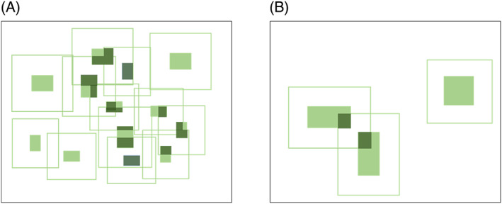
The total area contributing the species pool available to colonize a set of several small patches (A) is larger than the total area contributing the species pool available to colonize a set of few large patches of the same total area (B). Light‐coloured rectangles are patches. Boxes around them represent the areas from within which habitat can contribute colonists to the patches. Dark‐coloured rectangles are the areas of other habitat patches within the local landscape surrounding each patch.

(3). Predictions based on beta diversity

All of the SLOSS predictions discussed so far derive from assumptions about how extinction/mortality and colonization/immigration dynamics interact with sizes of individual patches and with sets of patches. In general, SL > SS is predicted when extinction dominates these dynamics, except when spreading‐of‐risk plays an important role in population dynamics. SS > SL is generally predicted when colonization/immigration dominates the dynamics. Considering these factors together, Ovaskainen (2002) predicted that an intermediate number of medium‐sized patches will often hold the most species.

A different set of SLOSS theory asks how the number of patches (for a given total habitat amount) is expected to affect beta diversity. Perhaps the simplest or null theory is the ‘geometric effect’, based on a cookie‐cutter analogy (May et al., ²⁰¹⁹). Here, the species occurring in a habitat patch are simply those that existed there before it became cut into a patch through habitat loss. When these pre‐existing species distributions are clumped or spatially autocorrelated, a given area cut into a large number of small patches will intersect more of these pre‐existing species distributions than when that area is cut into a small number of large patches, leading to higher beta diversity in SS and a prediction of SS > SL (May et al., ²⁰¹⁹; Fig. 2).

Fig 2.

When species distributions are clumped or spatially autocorrelated, a few large patches (A) will intersect (sample) fewer species than several small patches (B and C). Different colours represent different species within continuous habitat in a single ecoregion before habitat loss (large rectangles). Squares represent patches subsequently created by habitat loss. When the landscape extent (maximum distance between patch edges) is the same for few large and several small patches (A versus B), several small patches will cover the area more evenly and will therefore intersect more species: in A two large patches intersect three species while in B eight small patches intersect five species. This effect is accentuated if the several small patches are further apart than the few large patches: in C eight small patches intersect nine species compared to three species in A.

We consider the geometric effect a null expectation because most species distributions are clumped (Nekola & White, 1999; Tuomisto, Ruokolainen & Yli‐Halla, ²⁰⁰³; Seidler & Plotkin, ²⁰⁰⁶; Morlon et al., ²⁰⁰⁸; McGill, ^{2010, 2011}). Clumping can arise from intrinsic factors including limited dispersal from occupied sites creating population centres (Hubbell, 2001; Tuomisto et al., ²⁰⁰³), conspecific attraction (e.g. Vité & Francke, ¹⁹⁷⁶; Ramsay, Otter & Ratcliffe, ¹⁹⁹⁹; Schuck‐Paim & Alonso, ²⁰⁰¹; Peignier et al., ²⁰¹⁹), and philopatry (Weatherhead & Forbes, 1994). However, the main driver of clumped species distributions may be their responses to clumped or spatially autocorrelated micro‐habitats (e.g. soil type or microclimate). The ‘cookie‐cutter’ argument (above) also applies to micro‐habitats, and so we expect that a given area cut into a large number of small patches will intersect more micro‐habitats (higher across‐habitat heterogeneity) than when that area is cut into a small number of large patches. If species distributions are related to micro‐habitat distributions, this leads to a prediction of SS > SL due to higher beta diversity in SS (Lasky & Keitt, 2013). An exception to this argument would occur if large patches contain specific micro‐habitats that are absent from all small patches, as might occur for island systems where maximum elevation is higher on large than on small islands. Finally, spatially autocorrelated disturbances are predicted to increase the spatial clumping or autocorrelation of micro‐habitats and species distributions, accentuating beta diversity in SS and the tendency for SS > SL (Diamond, 1975; Simberloff & Gotelli, ¹⁹⁸⁴; Nekola & White, ²⁰⁰²; Kallimanis et al., ²⁰⁰⁵; Laurance et al., ²⁰⁰⁷; Lasky & Keitt, ²⁰¹³).

Note that the prediction of higher beta diversity across SS than SL does not assume or imply that small patches are further apart than large patches. Indeed, when the landscape size and the amount of habitat are held constant, there is no consistent difference between SS and SL in habitat spread, measured as maximum habitat edge‐to‐edge distance (Appendix S2). Spatial clumping of species distributions is nevertheless expected to lead to more species sampled over SS than SL because SS will cover a given area more evenly than SL, thus intersecting more micro‐habitats and more species distributions leading to higher beta diversity [compare Fig. 2A and B (Tscharntke et al., ²⁰⁰²; May et al., ²⁰¹⁹)].

If a set of several small patches happen to be more spread out than a set of a few large patches (e.g. Hill et al., ²⁰¹¹), beta diversity is predicted to increase even more over SS, due to even higher across‐habitat heterogeneity in SS than SL (Nekola & White, 1999; Morlon et al., ²⁰⁰⁸; Anderson et al., ²⁰¹¹; compare Fig. 2A and C). In other words, as pointed out early on by Higgs & Usher (1980), we can expect SS > SL if the proportional species overlap between patches is lower for SS than SL. However, increasing the distance among SS is also predicted to reduce inter‐patch movements, increasing patch isolation, and therefore to increase extinction dominance of extinction–colonization dynamics (Table 1). Thus, the spatial spread of SS is predicted to have two opposing effects: (i) decreasing inter‐patch movement potentially leading to SL > SS, and (ii) increasing across‐habitat heterogeneity and decreasing species overlap leading to higher beta diversity and SS > SL (Tjørve, 2010; Blowes & Connolly, ²⁰¹²; Arnillas et al., ²⁰¹⁷). Finally, higher beta diversity across SS than across SL may be accentuated over time following patch creation if different patches follow different successional trajectories (Laurance, 2002; Laurance et al., ²⁰⁰⁷; Ewers et al., ²⁰¹³; del Castillo, ²⁰¹⁵; Arroyo‐Rodriguez et al., ²⁰¹⁷).

III. RESEARCH AGENDA

Here we propose a research agenda for resolving the SLOSS dilemma. We first develop a hypothesis, the ‘SLOSS cube hypothesis’, that summarizes SLOSS predictions in combination with empirical SLOSS studies. We then use this hypothesis to propose an agenda for future empirical studies to ask, ‘are there any consistent, empirically demonstrated conditions that lead to SL > SS?’

(1). The SLOSS cube hypothesis

The major features of SLOSS predictions and data to date are illustrated in Fig. 3. To summarize the predictions: (i) arguments based on population processes generally predict SL > SS when between‐patch movements are assumed to be rare, such that variation in local (patch) extinctions dominates the extinction–colonization dynamic; (ii) an exception to this occurs where spreading‐of‐risk plays a large role in population persistence, leading to a prediction of SS > SL; (iii) arguments based on population processes generally predict SS > SL when between‐patch movements are assumed to be common such that variation in colonization dominates the extinction–colonization dynamic; and (iv) consideration of beta diversity and across‐habitat heterogeneity generally leads to predictions of SS > SL. Therefore, SLOSS predictions can be largely characterized by the combination of three variables: the frequency of between‐patch movements; the role of spreading‐of‐risk in landscape‐scale population persistence; and the level of species clumping indexed as across‐habitat heterogeneity. These are the three axes in Fig. 3.

Fig 3.

Illustration of the ‘SLOSS cube’, combining SLOSS‐relevant theory and empirical SLOSS studies. The axes are based on the theory and predictions summarized in Table 1. The proportional volumes of the three outcomes are based on their proportions found in a review of empirical SLOSS studies in which sampling effort was unbiased, i.e. sampling proportional to area (see fig. 2b in Fahrig, ²⁰²⁰): 50% SS > SL (yellow); 40% SL = SS (green); 10% SL > SS (blue). The SLOSS cube hypothesis predicts that SL > SS will dominate only when all of the following are true: between‐patch movement rate is low, the influence of spreading‐of‐risk on population dynamics is low, and across‐habitat heterogeneity is low, leading to low beta diversity.

To summarize empirical work to date based on classical SLOSS studies (Quinn & Harrison, 1988): about 50% of apparently unbiased (see Section III.2) empirical SLOSS studies find SS > SL and about 10% find SL > SS, while the remaining 40% find no difference (Fahrig, 2020). These proportions are represented as the coloured volumes in Fig. 3. Given the relative rarity of SL > SS results, the SLOSS cube hypothesis predicts that SL > SS will occur predictably only when all of the following are met: between‐patch movements are rare, the role of spreading‐of‐risk in landscape‐scale population dynamics is low, and across‐habitat heterogeneity and species clumping are low, reducing the role of beta diversity (blue volume in Fig. 3). The prediction that all three conditions must hold to obtain SL > SS derives not only from the relative rarity of SL > SS, but also from preliminary summaries of relevant empirical work suggesting that when only one or two of these conditions holds we still find a predominance of SS > SL (reviewed in Fahrig, ²⁰²⁰). In particular, SS > SL is more common than SL > SS in situations with higher matrix hostility, suggesting that low between‐patch movement rate alone is insufficient to produce SL > SS reliably. In addition, many cases of SS > SL occur in situations where across‐habitat heterogeneity is low (Fahrig, 2020), suggesting that low spatial autocorrelation in environmental characteristics (leading to low beta diversity) alone is not sufficient to produce SL > SS reliably. Furthermore, a recent microcosm experiment involving 11 species over multiple trophic levels found SS > SL, even though there was no movement at all between patches and all habitat was homogeneous (Hammill & Clements, 2020). Extinction rates were lower across SS than SL, leading to SS > SL. This finding suggests that the effect of spreading‐of‐risk may be stronger than is often assumed and may be sufficient to result in SS > SL even when between‐patch movement is very low and SS are not more heterogeneous than SL. Consistent with this we note that 16 of 20 SLOSS comparisons from island systems reviewed in Fahrig (2020) found SS > SL. In these systems, between‐patch movement is low and SL are likely more heterogeneous than SS (see Section II.3), again suggesting a strong role of spreading‐of‐risk in creating SS > SL. Nevertheless, the combination of factors – low between‐patch movement, low role of spreading‐of‐risk, and low across‐habitat heterogeneity – has not yet been explicitly tested across a range of systems.

(2). Testing the SLOSS cube hypothesis

Testing the SLOSS cube hypothesis will require a large number of individual empirical studies, where each study represents a point within the cube in Fig. 3. For each study, four variables should be estimated: (i) the frequency of between‐patch movements, (ii) the degree to which spreading‐of‐risk is important for landscape‐scale population persistence, (iii) the level of across‐habitat heterogeneity; and (iv) gamma diversity over different landscapes characterized by SS versus SL. Note empirical tests will measure across‐habitat heterogeneity rather than spatial clumping of species because estimating the spatial distribution of multiple species over multiple landscapes (see Section II.3) is generally not feasible. By contrast, across‐habitat heterogeneity is one of the major reasons for clumped species distributions, and can be measured from continuous raster maps based on remotely sensed data, using surface metrics (Riva & Nielsen ²⁰²⁰) such as metrics of spatial variance of the normalized difference vegetation index (NDVI; e.g. Duro et al., ²⁰¹⁴).

The frequency of between‐patch movements is unknown and hard to measure for nearly all species groups and regions. While relative innate mobility of different species groups can often be estimated using morphological or life‐history correlates (Bowman, Jaeger & Fahrig, ^2002b ; Stevens et al., ²⁰¹⁴; Beckman, Bullock & Salguero‐Gόmez, ²⁰¹⁸), the realized frequency of between‐patch movements is related not only to innate mobility but also to landscape attributes such as habitat configuration and matrix quality. Therefore, we propose a combination of two steps for selecting species groups with low (or high) between‐patch movement frequency in the selected region. First, species groups would be identified as low or high innate mobility based on morphology and life‐history traits such as wing presence/absence, territory size, etc. The purpose of the second step is then to confirm that, in the selected region, the low‐mobility group does in fact show low between‐patch movement and/or the high‐mobility group does in fact show high between‐patch movement. This can be done indirectly by comparing mean species density (number of species per sample site) of the mobility group in landscapes with SS versus SL. If, for the low mobility group, movement is lower between patches than within patches in the selected region, then we should find lower mean species density in sample sites across a landscape with SS than across a landscape with SL (Tjørve, 2010).

The role that spreading‐of‐risk plays in landscape‐scale population persistence is also unknown for most groups of species. However, it should be possible roughly to categorize species groups into those that are likely to benefit from spreading‐of‐risk versus those that are not. Those that might benefit from spreading‐of‐risk would include: groups under strong top‐down control from predators/parasitoids; groups of weaker competitors; and groups subject to frequent local disturbances (see Section II.1). These conditions do not guarantee that the species group benefits from spreading‐of‐risk. However, the absence of all three of these conditions would be a strong indicator of a species group that does not benefit from spreading‐of‐risk, and therefore of a potential species group to include in tests of the question, ‘are there any consistent, empirically demonstrated conditions that lead to SL > SS?’ as illustrated in Fig. 3.

Here we describe the characteristics of individual empirical studies that together would test the SLOSS cube hypothesis (Fig. 3). Importantly, each study should be based on randomly distributed samples within each of multiple landscapes (Fig. 4), rather than using the classical SLOSS approach (Quinn & Harrison, 1988) where species lists are combined across subsets of patches within the same landscape. Using random samples across multiple landscapes is preferable because it avoids two problems inherent in many empirical SLOSS studies to date.

Fig 4.

SLOSS can be evaluated by comparing cumulative species richness across the same number of sample sites (black squares) randomly placed within habitat (green rectangles) in multiple landscapes of the same size, each containing the same total area of habitat, but distributed in different numbers and sizes of patches. Two example landscapes are shown here, each with 10 sample sites placed randomly in habitat. Note that when the landscape has many small patches, some will not be sampled. This is not a problem because the unit of analysis in such a study is the landscape, not the patch.

First, using multiple landscapes avoids the problem that when all sampled patches are within the same landscape, large patches are intermixed with small patches. This classical study design is inconsistent with the inferences actually made from those studies, which are about whether many small patches (alone) have more or fewer species than few large patches (alone). In addition, when SLOSS is evaluated using subsets of intermixed patches, the link between the data and several of the mechanisms in Table 1 becomes unclear. For example, it is not clear how the spreading‐of‐risk of predation over SS would play out in a landscape in which small and large patches are intermixed. As another example, when small and large patches are intermixed, the amount of habitat contributing the species pools for colonization of SS versus SL (Fig. 2) includes portions of large and small patches within the local landscapes, and so the link between SLOSS and landscape moderation effects becomes unclear. Therefore, future empirical studies should sample species in multiple landscapes, each containing either SS or SL (Fig. 4), rather than subsets of SS or SL drawn from within a single landscape. The total habitat amount should be either the same across sampled landscapes, or at least habitat amount should be uncorrelated with the number of patches.

The second reason that using random samples across multiple landscapes is preferable to the classical SLOSS study design is that it avoids the problem that sampling is often biased in favour of SS (Gavish, Ziv & Rosenzweig, 2012). Small patches often have more sample sites per area than large patches, which means that the probability of detecting a given species is higher across SS than SL. Only about half of all SLOSS studies to date have apparently unbiased sampling effort (Fahrig, 2020). This is due to logistical constraints when the range of patch sizes is large. For example, if patches range in size from 5 ha to 1000 ha then, for equal sampling effort, the smallest possible number of sample sites in a 1000‐ha patch would be 200, assuming there is only one sample site per 5‐ha patch. For many species groups, such sample sizes would be impossible to accomplish. We note that if sampling effort information is available, patch size dependence on sampling effort can be estimated and controlled for in statistical models when using existing data (e.g. Deane et al., ²⁰²⁰). However, when designing a new empirical SLOSS study, the sampling effort problem can be best avoided by using random samples across multiple landscapes (Fig. 4). Cumulative number of species (gamma diversity) can then be directly compared for landscapes with SS versus landscapes with SL (Fig. 4).

Studies that together would test the SLOSS cube hypothesis should, ideally, have the following additional attributes. First, all sample landscapes in a given study (one point in the cube; Fig. 3) should have the same spatial extent and samples should be randomly distributed within the habitat in each landscape, with the number of samples in proportion to total habitat amount in the landscape. All sample landscapes within a study should also be within a single ecoregion, to ensure the same overall species pool, and the species included in the surveyed group should be those that are mainly associated with the particular habitat type studied. Here, significant attention should be paid to the definition of ‘habitat’. For example, single trees may not be habitat patches for species groups that rely on humid forest understorey conditions; however, single trees can be habitat patches for wood‐boring beetles. In addition, confounding of other variables with the SL versus SS comparison should be avoided. For example, an apparent pattern of SS > SL could be created where larger patches are more intensively managed or where smaller patches have more varied management approaches (e.g. grazed, mown, abandoned) than large ones, e.g. due to different ownership of different patches (Rösch et al., ²⁰¹⁵). Conversely, an apparent pattern of SL > SS could be created where small patches are more disturbed by humans than are large patches (e.g. Barlow et al., ²⁰¹⁶). In addition, the spatial pattern of patches should have been already in place for several generations of the surveyed species group. This is to ensure: (i) dissipation of transient positive fragmentation effects caused by a crowding effect on small patches following patch creation (Grez et al., ²⁰⁰⁴), and (ii) sufficient time for any extinctions to play out (Figueiredo et al., ²⁰¹⁹). Finally, differences in species detectability (MacKenzie et al., ²⁰⁰²) between SS and SL should be estimated and accounted for if present. We reiterate that these are the ideal attributes for each study; where particular attributes cannot be controlled through study design, it may often be possible to control for them in statistical models.

(3). Method for determining whether there are consistent, empirically demonstrated conditions that lead to SL > SS

As discussed above, the SL > SS principle continues to guide conservation decision‐making in many situations, despite lack of empirical support for it as a general principle. To resolve this dilemma, we need to determine whether SL > SS is in fact a valid principle in a predictable set of conditions. The principle could then be reworded as, ‘in general SL > SS whenever conditions x hold.’ Such conditions have been suggested (Table 1; summarized in Fig. 3) but to date there is little supporting empirical evidence. Therefore, resolving the SLOSS dilemma means addressing the question, ‘are there any consistent, empirically demonstrated conditions that lead to SL > SS?’

Addressing this question requires multiple empirical tests, using appropriate study designs, focused on species groups and environments where between‐patch movements are rare, spreading‐of‐risk is likely unimportant, and habitat is relatively homogeneous. In other words, studies should focus on the blue portion of the SLOSS cube in Fig. 3. If the majority of studies in this space find SL > SS, then we can conclude that the SL > SS principle is generally valid in those conditions. As discussed above, estimates of realized interpatch movement rates for groups of species are usually not available for a given region, but movement rates should be low when patches are very far apart or the matrix is hostile, or when the species group is comprised of sedentary species. Therefore, SLOSS tests should focus on regions where (i) habitat is rare, i.e. patches – both large and small – are far apart relative to the dispersal range of the species group, (ii) habitat is spatially homogeneous, and (iii) the matrix is hostile (e.g. urban areas, high‐intensity agriculture). The groups of species selected should be those assumed to have low innate mobility, and those for whom spreading‐of‐risk likely plays a minor role in population dynamics, i.e. stronger competitors under bottom‐up control that are not subject to frequent local disturbances (see Section II.1). Once a region and a species group have been selected, multiple sample landscapes should be selected within that region, that vary in the numbers and sizes of patches and do not vary in total habitat amount (Fig. 4), or for which there is no relationship between habitat amount and the numbers and sizes of patches across the landscapes. Sample sites should then be randomly placed in the habitat within each landscape, and the species group sampled at each site. Average species density (mean number of species per site) should be compared between SS and SL to confirm the assumption of low between‐patch movement in the selected region (see Section III.2). Total species richness (gamma diversity) should then be estimated across the habitat in each landscape to determine whether there are more species in landscapes with SL than SS.

(4). Note on negative edge effects and SLOSS

As indicated in Table 1, habitat interior species, i.e. those that show negative edge effects, should be particularly susceptible to the effects of patch size on extinction probability. In addition, they may have low mobility between patches if they are averse to leaving interior habitat and entering the matrix. For this reason, patch‐scale evidence of negative edge effects on a species group is often taken as evidence of SL > SS for that group (Fletcher et al., ²⁰¹⁸). However, we note that SL > SS cannot be directly inferred for groups of habitat interior species based only on patch‐scale evidence. Such an inference would entail cross‐scale extrapolation (Wiens, 1989) from local edge effects to landscape‐scale effects. This extrapolation is a prediction that must be tested at a landscape scale because other mechanisms in Table 1, operating at a landscape scale, may outweigh negative local edge effects in influencing species richness across a landscape (Fahrig et al., ²⁰¹⁹). Such tests would compare gamma diversity of species groups known to show negative edge effects (and thus assumed to fall into the blue portion of the SLOSS cube in Fig. 3), across multiple landscapes as in Fig. 4.

We note further that such studies will need to estimate gamma diversity, not species richness at a sample site, i.e. species density. For example, Püttker et al. (2020) documented negative effects on species density of edge density in the local landscapes surrounding sample sites. The observed reductions in local richness cannot be directly extrapolated to infer SL > SS because other mechanisms, such as higher beta diversity across SS than SL, might outweigh the negative effect of edge density when species richness is measured over the landscape. Again, extrapolation to SL > SS needs to be tested by comparing species richness (gamma diversity) across multiple landscapes with different numbers and sizes of patches.

(5). Need for many studies

Here we emphasize that a single study on a particular species group in a particular region cannot answer the question ‘are there consistent, empirically demonstrated conditions that lead to SL > SS?’ SL > SS was conceived and is used as a general principle. We know it is not universally valid, because most empirical studies do not support it. However, it may still apply in general when certain conditions hold, specifically the combination of low between‐patch movement, low spreading‐of‐risk, and low across‐habitat heterogeneity. Testing this prediction will require multiple studies on a range of taxa and regions that match these conditions (Seibold et al., ²⁰¹⁸). SL > SS would be upheld as a principle if we find more species in habitat within landscapes with SL than in those with SS, in most of these studies.

IV. DISCUSSION

In one sense, by proposing this research agenda, we are reviving a debate that most ecologists had set aside. Most ecologists believe that there is no general SLOSS principle and that each case must be evaluated individually. But at the same time the idea persists that the SL > SS principle is generally valid under some conditions (Table 1), such as for groups of habitat‐interior species and in landscapes with low matrix quality (Pfeifer et al., ²⁰¹⁷; Fletcher et al., ²⁰¹⁸), and that these are the conditions where biodiversity is most threatened. However, empirical tests to date do not generally support the SL > SS principle even in these conditions. If anything, the evidence so far suggests the reverse (Fahrig, 2020), although the number of tests is much smaller than needed for evaluating a general principle. We suggest that this contradiction needs to be resolved for the sake of biodiversity conservation, and we propose our research agenda as a path to resolving it.

We acknowledge, however, that testing the SLOSS cube hypotheses will be challenging, for three major reasons. First, each study requires sufficient information about the species in the study group, such as their primary habitat associations, their mobility, and their dominant interactions with other species. The second major challenge will be selecting multiple, appropriately sized landscapes to create cross‐landscape variation in the number of patches while minimizing potential confounding variables. Third, once the species group and landscapes have been selected, sampling many species across many sites within each of many landscapes will present a large logistical challenge. Nevertheless, we hope that the SLOSS cube hypothesis will allow researchers to identify study systems that are not only feasible but also will provide informative tests of the hypothesis. Recent improvements to habitat information through remote sensing developments (Skidmore et al., ²⁰²¹), and large‐scale species sampling through community science (e.g. eBird, eButterfly) and through large, collaborative research efforts (e.g. Sirami et al., ²⁰¹⁹) should increase the feasibility of tests going forward. Creative experimental approaches such as microcosm experiments (e.g. Hammill & Clements, ²⁰²⁰) may also be particularly useful for controlling the large number of factors involved. Overall, we recommend that particular effort should be put toward identifying and studying systems that are likely in the blue portion of Fig. 3, to focus tests on the question, ‘are there consistent, empirically demonstrated conditions leading to SL > SS?’

There are two possible outcomes of research aimed at testing the SLOSS cube hypothesis. First, empirical studies might generally support the hypothesis. This would have different implications for conservation decision‐making, depending on the conservation goal. In situations where the goal is general conservation of biodiversity, support for the hypothesis would suggest that a mixed strategy of mainly small patches and a few large patches would maximize biodiversity, as suggested by Arroyo‐Rodríguez et al. (2020). On the other hand, when the goal is the conservation of a particular species group, then support for the hypothesis would indicate what research the conservation agency needs to carry out to determine whether the particular conditions in their system fall within the range of conditions where SL > SS is valid. In particular, does the level of between‐patch movement, the role of spreading‐of‐risk, and the level of across‐habitat heterogeneity place the system within the blue portion of the SLOSS cube in Fig. 3? If so then, for biodiversity conservation, large patches should be prioritized and small patches should be down‐weighted, but if not, then total habitat amount and its heterogeneity should be maximized irrespective of the sizes of patches comprising it.

The second possible outcome of the proposed research agenda is that the majority of studies find either SS > SL or SL = SS throughout the SLOSS cube in Fig. 3, even when between‐patch movement, spreading‐of‐risk, and across‐habitat heterogeneity are all low. In that case, we should conclude that the SLOSS cube hypothesis is not supported, i.e. SL > SS is not a general principle under any predictable conditions, and therefore it should not be used in conservation planning. Two lines of evidence suggest this outcome is at least possible. First, reviews of empirical studies to date have not found predictable conditions leading to SL > SS; the majority of results so far find SS > SL for habitat specialists, when the matrix is hostile, when habitat amount is low, and when across‐habitat heterogeneity is low (reviewed in Fahrig, ^{2017a , 2020}). Second, simulations by Fronhofer et al. (2012) suggest that the main mechanism proposed to lead to SL > SS – extinction–colonization dynamics dominated by variation in extinction rate – is likely very rare in nature. Fronhofer et al. (2012) predict this situation is usually evolutionarily unstable, with systems either becoming extinct or between‐patch movement rates increasing such that variation in extinction rate no longer drives the extinction–colonization dynamic.

We note that the idea that the SL > SS principle could be abandoned seems to fly in the face of the fact that there are documented empirical cases of SL > SS. Nevertheless, given the small number of these cases to date, if they do not occur in predictable conditions, then we would not be able to discount the possibility that they are due to statistical chance alone. In a review of effects of fragmentation per se (of which SLOSS is one component), Fahrig (2017a ) found that 24% of significant fragmentation effects were negative (i.e. SL > SS in the context of SLOSS). However, fewer than 30% of all effects were significant, suggesting that fewer than 7.2% of all effects are significantly negative. Furthermore, documented reporting biases (Fahrig, ^2017b ) reduce this estimate to about 3–4.2% of all tests. Thus, if it turns out that there are no empirically demonstrated, consistent conditions leading to SL > SS, then it would be reasonable to infer that the few SL > SS findings to date may be due to statistical chance alone.

If there are no consistent conditions leading to SL > SS, this would confirm that small habitat patches have the same or greater biodiversity value as the same area of habitat in large patches. It would also mean that the overall goal for conservation should be to preserve or restore as much area as possible of each natural habitat type within a given ecoregion, intersecting the distributions of as many species as possible, irrespective of the patch sizes within which the habitat is distributed, as long as the patches are large enough to function as habitat for the species group (Rösch et al., ²⁰¹⁵). It would also call into question conservation planning algorithms that minimize total boundary length, because their solutions favour larger, more compact areas, at the expense of the total area included in the ‘optimal’ solution (Stewart & Possingham, 2005; Hermosa et al., ²⁰¹¹). Removing the constraint that a given amount of habitat must be in large contiguous patches would increase options for conservation, especially in regions dominated by people where there are no large, contiguous natural areas remaining and where many taxa are declining (e.g. van Klink et al., ²⁰²⁰). Collections of small reserves such as small forest patches and riparian and wetland buffers could have high biodiversity value in such ecoregions. This would provide a rationale for local small‐scale conservation efforts, both public and private (Monteferri, 2019; Shumba et al., ²⁰²⁰).

We note that SLOSS predictions (Table 1) and metacommunity theory (Leibold et al., ²⁰⁰⁴) rely on similar mechanisms. However, to our knowledge, metacommunity theory has not been explicitly used to predict the outcome of SLOSS. In their recent review of the link between metacommunity theory and biodiversity conservation, Chase et al. (2020, p. 8) suggest that the “debate in the literature about the influence of habitat fragmentation [of which SLOSS is one element] on biodiversity .. is largely misplaced until one can gain a more definitive focus on the mechanisms being influenced and the scales at which those influences occur.” On the other hand, Fournier et al.'s (2017) proposed general theory of metacommunity ecology, while not explicitly aimed at the SLOSS question, indirectly supports our SLOSS cube hypothesis. Fournier et al. (2017) modelled the independent and combined effects on species coexistence (here analogous to species richness) of: (i) habitat aggregation (analogous to the SS to SL gradient), (ii) aggregation of environmental conditions (analogous to across‐habitat heterogeneity), and (iii) connectivity (analogous to the frequency of between‐patch movements). They predict maximum species coexistence under the combined conditions of low habitat aggregation (SS), high across‐habitat heterogeneity, and high between‐patch movement frequency. It therefore appears that the SLOSS cube hypothesis is compatible with general metacommunity theory, although a more formal evaluation is needed.

We recognize that even if there is no evidence for SL > SS as a general principle, this will not necessarily translate into a higher priority for preservation of SS than SL in a given situation. As mentioned above, factors other than total species richness enter into decisions about habitat preservation and restoration. For example, maintenance of some ecological processes may require large areas, and the perception of wildness may depend on the size of the ecosystem (Perino et al., ²⁰¹⁹). In addition, a few large areas may be easier to manage than many small ones, as suggested by Higgs & Usher (1980). Finally, when the goal is to conserve a particular threatened species, preserving a large, contiguous area may often be more effective than preserving several small ones. For example, for species that are prone to be killed or removed legally or illegally when encountered or discovered by people (e.g. top predators or high‐value trees), large contiguous natural areas may be the only way to ensure that such encounters are rare (e.g. Müller et al., ²⁰¹⁴). Nevertheless, in such situations, prioritizing preservation of few large areas over many small ones would be taken not because the SL > SS principle is valid, but in spite of the fact that it is not.

We also note that, if there are no consistent, empirically demonstrated conditions leading to SL > SS, this does not invalidate the mechanisms proposed in Table 1. Rather, it would mean that the mechanisms predicting SS > SL outweigh the mechanisms predicting SL > SS in nature. Put differently, it would mean that, for a mechanism to result in SL > SS, the conditions would need to be so extreme – e.g. perfectly homogeneous habitat and essentially no between‐patch movement – that they are almost never observed except in models.

We emphasize that SLOSS is explicitly not about the role of habitat amount. Rather, it is about the influence of the pattern or configuration of a given amount of habitat (several small versus few large patches). Habitat loss is the main cause of species declines, and so habitat preservation and restoration are the top priorities for biodiversity conservation. If, in a particular situation, a choice is presented between conserving one large patch versus several small patches, but the small patches have much less habitat in total, then the decision should be to conserve the large patch. For example, in the Steigerwald forest in Southern Germany there is an ongoing discussion about establishing a national park of 10000 ha versus protecting a set of smaller areas of about 5000 ha in total. Here, the large national park would probably be more effective for biodiversity conservation, because the total habitat preserved would be twice that of the set of small patches.

We also emphasize that we would never recommend the intentional fragmentation of what is now continuous habitat. Such areas are increasingly rare globally (Watson et al., ²⁰¹⁶), and their fragmentation would entail loss of habitat. Large protected areas should remain, and to the extent possible, so should remaining large unprotected tracts of contiguous habitat.

V. CONCLUSIONS

1. While most empirical SLOSS studies find SS > SL, many conservation agencies prioritize protection of large, contiguous areas of habitat, while small patches of natural habitat are less likely to be protected.

2. We suggest that this dilemma can be resolved by asking, ‘are there consistent, empirically demonstrated conditions leading to SL > SS?’

3. Most predictions of SL > SS depend on the assumption that variation in extinction rate dominates the outcome of the extinction–colonization dynamic. This should occur when populations in separate patches are largely independent of each other due to low between‐patch movements, and when species differ in minimum patch size requirements, leading to a strong pattern of species nestedness with patch size.

4. However, even when variation in extinction rate dominates the outcome of the extinction–colonization dynamic, theory can predict SS > SL if extinctions are caused by antagonistic species or disturbances, leading to spreading‐of‐risk of landscape‐scale extinction across SS.

5. SS > SL is also predicted when variation in colonization dominates the outcome of the extinction–colonization dynamic, due to higher immigration rates for SS than SL, and larger species pools in the proximity of SS than SL.

6. Considerations of beta diversity also lead to predictions of SS > SL because SS will intersect or ‘sample’ more micro‐habitats and more species distributions when micro‐habitats and species are clumped or spatially autocorrelated.

7. We summarize these predictions into the SLOSS cube hypothesis, where the combination of three axes – between‐patch movement, the role of spreading‐of‐risk for landscape‐scale population persistence, and across‐habitat heterogeneity – predicts the SLOSS outcome.

8. We use the SLOSS cube hypothesis, combined with existing SLOSS empirical evidence, to predict SL > SS only when all of the following are true: between‐patch movement is low, spreading‐of‐risk is relatively unimportant for landscape‐scale population persistence, and large‐scale across‐habitat heterogeneity is low.

9. Testing this prediction will require a large number of studies targeted at species groups and regions where these three conditions hold.

10. These studies should be designed such that samples are randomly distributed across habitat over multiple equal‐sized landscapes containing different numbers and sizes of patches but the same total amount of habitat.

11. If the majority of studies in these conditions show more species in landscapes with few large than several small patches then this will delineate the situations in which the SL > SS principle can be included as a criterion in reserve design.

12. On the other hand, if the majority of studies in these conditions find more species in landscapes with several small patches, or no difference, then the SL > SS principle should be abandoned.

Supporting information

Appendix S1. Use of the term ‘SLOSS debate’ as a proportion of all English‐language literature, per year since 1980, estimated using Google Ngram (Michel et al., ²⁰¹¹).

Appendix S2. Habitat extent (maximum distance between habitat edges in a landscape) versus number of patches in the landscape, for landscapes within each of 32 studies included in the main analysis in Watling et al. (2020).

REFERENCES

- Amarasekare, P. & Nisbet, R. M. (2001). Spatial heterogeneity, source‐sink dynamics, and the local coexistence of competing species. American Naturalist 158, 572–584. [DOI] [PubMed] [Google Scholar]
- Anderson, M. J. , Crist, T. O. , Chase, J. M. , Vellend, M. , Inouye, B. D. , Freestone, A. L. , Sanders, N. J. , Cornell, H. V. , Comita, L. S. , Davies, K. F. , Harrison, S. P. , Kraft, N. J. B. , Stegen, J. C. & Swenson, N. G. (2011). Navigating the multiple meanings of β diversity: a roadmap for the practicing ecologist. Ecology Letters 14, 19–28. [DOI] [PubMed] [Google Scholar]
- Andrewartha, H. G. (1984). Ecology at the cross‐roads. Australian Journal of Ecology 9, 1–3. [Google Scholar]
- Armsworth, P. R. , Jackson, H. B. , Cho, S.‐H. , Clark, M. , Fargione, J. E. , Iacona, G. D. , Kim, T. , Larson, E. R. , Minney, T. & Sutton, N. A. (2018). Is conservation right to go big? Protected area size and conservation return‐on‐investment. Biological Conservation 225, 229–236. [Google Scholar]
- Arnillas, C. A. , Tovar, C. , Cadotte, M. W. & Buytaert, W. (2017). From patches to richness: assessing the potential impact of landscape transformation on biodiversity. Ecosphere 8, e02004. [Google Scholar]
- Arroyo‐Rodríguez, V. , Fahrig, L. , Tabarelli, M. , Watling, J. I. , Tischendorf, L. , Benchimol, M. , Cazetta, E. , Faria, D. , Leal, I. R. , Melo, F. P. L. , Morante‐Filho, J. C. , Santos, B. A. , Arasa‐Gisbert, R. , Arce‐Peña, N. , Cervantes‐López, M. J. , et al. (2020). Designing optimal human‐modified landscapes for forest biodiversity conservation. Ecology Letters 23, 1404–1420. [DOI] [PubMed] [Google Scholar]
- Arroyo‐Rodríguez, V. , Melo, F. P. L. , Martínez‐Ramos, M. , Bongers, F. , Chazdon, R. L. , Meave, J. A. , Norden, N. , Santos, B. A. , Leal, I. R. & Tabarelli, M. (2017). Multiple successional pathways in human‐modified tropical landscapes: new insights from forest succession, forest fragmentation and landscape ecology research. Biological Reviews 92, 326–340. [DOI] [PubMed] [Google Scholar]
- Atmar, W. & Patterson, B. D. (1993). The measure of order and disorder in the distribution of species in fragmented habitat. Oecologia 96, 373–382. [DOI] [PubMed] [Google Scholar]
- Barlow, J. , Lennox, G. D. , Ferreira, J. , Berenguer, E. , Lees, A. C. , Mac Nally, R. , Thomson, J. R. , Frosini de Barros Ferraz, S. , Louzada, J. , Fonseca Oliveira, V. H. , Parry, L. , Ribeiro de Castro Solar, R. , Vieira, I. C. G. , Aragão, L. E. O. C. , et al. (2016). Anthropogenic disturbance in tropical forests can double biodiversity loss from deforestation. Nature 535, 144–147. [DOI] [PubMed] [Google Scholar]
- Beckman, N. G. , Bullock, J. M. & Salguero‐Gómez, R. (2018). High dispersal ability is related to fast life‐history strategies. Journal of Ecology 106, 1349–1362. [Google Scholar]
- Ben‐Hur, E. & Kadmon, R. (2020). Heterogeneity‐diversity relationships in sessile organisms: a unified framework. Ecology Letters 23, 193–207. [DOI] [PubMed] [Google Scholar]
- Blake, J. G. & Karr, J. R. (1984). Species composition of bird communities and the conservation benefit of large versus small forests. Biological Conservation 30, 173–187. [Google Scholar]
- Blowes, S. A. & Connolly, S. R. (2012). Risk spreading, connectivity, and optimal reserve spacing. Ecological Applications 22, 311–321. [DOI] [PubMed] [Google Scholar]
- Bowman, J. , Cappuccino, N. & Fahrig, L. (2002a). Patch size and population density: the effect of immigration behavior. Conservation Ecology 6, art 9. [Google Scholar]
- Bowman, J. , Jaeger, J. A. G. & Fahrig, L. (2002b). Dispersal distance of mammals is proportional to home range size. Ecology 83, 2049–2055. [Google Scholar]
- Brown, E. , Dudley, N. , Lindhe, A. , Muhtaman, D. R. , Stewart, C. & Synnott, T. (eds.). (2013) (October). Common Guidance for the Identification of High Conservation Values. HCV Resource Network. [Google Scholar]
- Burkey, T. V. (1989). Extinction in nature reserves: the effect of fragmentation and the importance of migration between reserve fragments. Oikos 55, 75–81. [Google Scholar]
- Chase, J. M. , Jeliazkov, A. , Ladouceur, E. & Viana, D. (2020). Biodiversity conservation through the lens of metacommunity ecology. Annals of the New York Academy of Sciences 1469, 86–104. [DOI] [PubMed] [Google Scholar]
- Cole, B. J. (1981). Colonizing abilities, island size, and the number of species on archipelagoes. American Naturalist 117, 629–638. [Google Scholar]
- CONAFOR (2021). Reglas de Operación del Programa Apoyos para el Desarrollo Forestal Sustentable 2021. Diario Oficial de la Federación (DOF). https://www.conafor.gob.mx/apoyos/index.php/inicio/app_apoyos#/detalle/2021/92 [Google Scholar]
- Deane, D. C. , Nozohourmehrabad, P. , Boyce, S. D. & He, F. (2020). Quantifying factors for understanding why several small patches host more species than a single large patch. Biological Conservation 249, e108711. [Google Scholar]
- del Castillo, R. F. (2015). A conceptual framework to describe the ecology of fragmented landscapes and implications for conservation and management. Ecological Applications 25, 1447–1455. [DOI] [PubMed] [Google Scholar]
- den Boer, P. J. (1968). Spreading of risk and stabilization of animal numbers. Acta Biotheoretica 18, 165–194. [DOI] [PubMed] [Google Scholar]
- Diamond, J. M. (1975). The island dilemma: lessons of modern geographic studies for the design of natural reserves. Biological Conservation 7, 129–146. [Google Scholar]
- Diamond, J. M. (1976). Island biogeography and conservation: strategy and limitations. Science 193, 1027–1029. [DOI] [PubMed] [Google Scholar]
- Duelli, P. (1997). Biodiversity evaluation in agricultural landscapes: an approach at two different scales. Agriculture, Ecosystems and Environment 62, 81–91. [Google Scholar]
- Dunning, J. B. , Danielson, B. J. & Pulliam, H. R. (1992). Ecological processes that affect populations in complex landscapes. Oikos 65, 169–175. [Google Scholar]
- Duro, D. C. , Girard, J. , King, D. J. , Fahrig, L. , Mitchell, S. , Lindsay, K. & Tischendorf, L. (2014). Predicting species diversity in agricultural environments using Landsat TM‐based imagery. Remote Sensing of Environment 144, 214–225. [Google Scholar]
- Edwards, D. P. , Fisher, B. & Wilcove, D. S. (2012). High conservation value or high confusion value? Sustainable agriculture and biodiversity conservation in the tropics. Conservation Letters 5, 20–27. [Google Scholar]
- Etienne, R. S. & Heesterbeek, J. A. P. (2000). On optimal size and number of reserves for metapopulation persistence. Journal of Theoretical Biology 203, 33–50. [DOI] [PubMed] [Google Scholar]
- Europarc Federation (2013). Wild Europe. A working definition of European wilderness and wild areas . https://www.europarc.org/wp-content/uploads/2015/05/a-working-definition-of-european-wilderness-and-wild-areas.pdf Accessed 17.06.2020.
- Ewers, R. M. , Didham, R. K. , Pearse, W. D. , Lefebvre, V. , Rosa, I. M. D. , Carreiras, J. M. B. , Lucas, R. M. & Reuman, D. C. (2013). Using landscape history to predict biodiversity patterns in fragmented landscapes. Ecology Letters 16, 1221–1233. [DOI] [PMC free article] [PubMed] [Google Scholar]
- Fahrig, L. (1998). When does fragmentation of breeding habitat affect population survival? Ecological Modelling 105, 273–292. [Google Scholar]
- Fahrig, L. (2002). Effect of habitat fragmentation on the extinction threshold: a synthesis. Ecological Applications 12, 346–353. [Google Scholar]
- Fahrig, L. (2013). Rethinking patch size and isolation effects: the habitat amount hypothesis. Journal of Biogeography 40, 1649–1663. [Google Scholar]
- Fahrig, L. (2017a). Ecological responses to habitat fragmentation per se. Annual Review of Ecology, Evolution, and Systematics 48, 1–23. [Google Scholar]
- Fahrig, L. (2017b). Forty years of bias in habitat fragmentation research. In Effective Conservation Science: Data Not Dogma (eds Kareiva P., Silliman B. and Marvier M.), pp. 32–38. Oxford University Press, Oxford. [Google Scholar]
- Fahrig, L. (2020). Why do several small patches hold more species than few large patches? Global Ecology and Biogeography 29, 615–628. [Google Scholar]
- Fahrig, L. , Arroyo‐Rodríguez, V. , Bennett, J. R. , Boucher‐Lalonde, V. , Cazetta, E. , Currie, D. J. , Eigenbrod, F. , Ford, A. T. , Harrison, S. P. , Jaeger, J. A. G. , Koper, N. , Martin, A. E. , Martin, J.‐L. , Metzger, J. P. , Morrison, P. , et al. (2019). Is habitat fragmentation bad for biodiversity? Biological Conservation 230, 179–186. [Google Scholar]
- Fahrig, L. , Baudry, J. , Brotons, L. , Burel, F. G. , Crist, T. O. , Fuller, R. J. , Sirami, C. , Siriwardena, G. M. & Martin, J.‐L. (2011). Functional landscape heterogeneity and animal biodiversity in agricultural landscapes. Ecology Letters 14, 101–112. [DOI] [PubMed] [Google Scholar]
- Figueiredo, L. , Krauss, J. , Steffan‐Dewenter, I. & Cabral, J. S. (2019). Understanding extinction debts: spatio–temporal scales, mechanisms and a roadmap for future research. Ecography 42, 1973–1990. [Google Scholar]
- Flather, C. H. & Bevers, M. (2002). Patchy reaction‐diffusion and population abundance: the relative importance of habitat amount and arrangement. American Naturalist 159, 40–56. [DOI] [PubMed] [Google Scholar]
- Fletcher, R. J. , Didham, R. K. , Banks‐Leite, C. , Barlow, J. , Ewers, R. M. , Rosindell, J. , Holt, R. D. , Gonzalez, A. , Pardini, R. , Damschen, E. I. , Melo, F. P. L. , Ries, L. , Prevedello, J. A. , Tscharntke, T. , Laurance, W. F. , et al. (2018). Is habitat fragmentation good for biodiversity? Biological Conservation 226, 9–15. [Google Scholar]
- Fournier, B. , Mouquet, N. , Leibold, M. A. & Gravel, D. (2017). An integrative framework of coexistence mechanisms in competitive metacommunities. Ecography 40, 630–641. [Google Scholar]
- Fovargue, R. , Bode, M. & Armsworth, P. R. (2018). Size and spacing rules can balance conservation and fishery management objectives for marine protected areas. Journal of Applied Ecology 55, 1050–1059. [Google Scholar]
- Fronhofer, E. A. , Kubisch, A. , Hilker, F. M. , Hovestadt, T. & Poethke, H. J. (2012). Why are metapopulations so rare? Ecology 93, 1967–1978. [DOI] [PubMed] [Google Scholar]
- Gagné, S. A. , Eigenbrod, F. , Bert, D. , Cunnington, G. M. , Olson, L. T. , Smith, A. C. & Fahrig, L. (2015). A simple landscape design framework for biodiversity conservation. Landscape and Urban Planning 136, 13–27. [Google Scholar]
- Gavish, Y. , Ziv, Y. & Rosenzweig, M. L. (2012). Decoupling fragmentation from habitat loss for spiders in patchy agricultural landscapes. Conservation Biology 26, 150–159. [DOI] [PubMed] [Google Scholar]
- Grez, A. , Zaviezo, T. , Tischendorf, L. & Fahrig, L. (2004). A transient, positive effect of habitat fragmentation on insect population densities. Oecologia 141, 444–451. [DOI] [PubMed] [Google Scholar]
- Hammill, E. & Clements, C. F. (2020). Imperfect detection alters the outcome of management strategies for protected areas. Ecology Letters 23, 682–691. [DOI] [PubMed] [Google Scholar]
- Hannah, L. , Roehrdanz, P. R. , Marquet, P. A. , Enquist, B. J. , Midgley, G. , Foden, W. , Lovett, J. C. , Corlett, R. T. , Corcoran, D. , Butchart, S. H. M. , Boyle, B. , Feng, X. , Maitner, B. , Fajardo, J. , McGill, B. J. , et al. (2020). 30% land conservation and climate action reduces tropical extinction risk by more than 50%. Ecography 43, 943–953. [Google Scholar]
- Heilmann‐Clausen, J. & Christensen, M. (2004). Does size matter? On the importance of various dead wood fractions for fungal diversity in Danish beech forests. Forest Ecology and Management 201, 105–117. [Google Scholar]
- Hermosa, V. , Linke, S. , Prenda, J. & Possingham, H. P. (2011). Addressing longitudinal connectivity in the systematic conservation planning of fresh waters. Freshwater Conservation Planning 56, 57–70. [Google Scholar]
- Hernández‐Ruedas, M. A. , Arroyo‐Rodríguez, V. , Meave, J. A. , Martínez‐Ramos, M. , Ibarra‐Manríquez, G. , Martínez, E. , Jamangapé, G. , Melo, F. P. L. & Santos, B. A. (2014). Conserving tropical tree diversity and forest structure: the value of small rainforest patches in moderately‐managed landscapes. PLoS One 9, e98931. [DOI] [PMC free article] [PubMed] [Google Scholar]
- Hernández‐Ruedas, M. A. , Arroyo‐Rodríguez, V. , Morante‐Filho, J. C. , Meave, J. A. & Martínez‐Ramos, M. (2018). Fragmentation and matrix contrast favor understory plants through negative cascading effects on a strong competitor palm. Ecological Applications 28, 1546–1553. [DOI] [PubMed] [Google Scholar]
- Higgs, A. J. & Usher, M. B. (1980). Should nature reserves be large or small? Nature 285, 568–569. [Google Scholar]
- Hill, J. K. , Gray, M. A. , Khen, C. V. , Benedick, S. , Tawatao, N. & Hamer, K. C. (2011). Ecological impacts of tropical forest fragmentation: how consistent are patterns in species richness and nestedness? Philosophical Transactions of the Royal Society B 366, 3265–3276. [DOI] [PMC free article] [PubMed] [Google Scholar]
- Hill, M. , Hassall, C. , Oertli, B. , Fahrig, L. , Robson, B. , Biggs, J. , Samways, M. J. , Usio, N. , Takamura, N. , Krishnaswamy, J. & Wood, P. J. (2018). New policy directions for global pond conservation. Conservation Letters 11, e12447. [Google Scholar]
- Hill, M. F. & Caswell, H. (1999). Habitat fragmentation and extinction thresholds on fractal landscapes. Ecology Letters 2, 121–127. [Google Scholar]
- Hubbell, S. P. (2001). The Unified Neutral Theory of Biodiversity and Biogeography. Princeton University Press, Princeton. [Google Scholar]
- Huffaker, C. B. (1958). Experimental studies on predation: dispersion factors and predator‐prey oscillations. Hilgardia 27, 795–835. [Google Scholar]
- Hutchinson, G. E. (1959). Homage to Santa Rosalia, or, why are there so many kinds of animals? American Naturalist 93, 145–159. [Google Scholar]
- IUCN (1980). World Conservation Strategy: Living Resource Conservation for Sustainable Development. International Union for Conservation of Nature and Natural Resources, Gland. [Google Scholar]
- Jagers, P. & Harding, K. C. (2009). Viability of small populations experiencing recurring catastrophes. Mathematical Population Studies 16, 177–198. [Google Scholar]
- Kallimanis, A. S. , Kunin, W. E. , Halley, J. M. & Sgardelis, S. P. (2005). Metapopulation extinction risk under spatially autocorrelated disturbance. Conservation Biology 19, 534–546. [Google Scholar]
- Kingsland, S. E. (2002). Creating a science of nature reserve design: perspectives from history. Environmental Modeling & Assessment 7, 61–69. [Google Scholar]
- Lasky, J. R. & Keitt, T. H. (2013). Reserve size and fragmentation alter community assembly, diversity, and dynamics. American Naturalist 182, E142–E160. [DOI] [PubMed] [Google Scholar]
- Laurance, W. F. (1991). Edge effects in tropical forest fragments: application of a model for the design of nature reserves. Biological Conservation 57, 205–219. [Google Scholar]
- Laurance, W. F. (2002). Hyperdynamism in fragmented habitats. Journal of Vegetation Science 13, 595–602. [Google Scholar]
- Laurance, W. F. , Nascimento, H. E. M. , Laurance, S. G. , Andrade, A. , Ewers, R. M. , Harms, K. E. , Luizão, R. C. C. & Ribeiro, J. E. (2007). Habitat fragmentation, variable edge effects, and the landscape‐divergence hypothesis. PLoS One 2, e1017. [DOI] [PMC free article] [PubMed] [Google Scholar]
- Leibold, M. A. , Holyoak, M. , Mouquet, N. , Amarasekare, P. , Chase, J. M. , Hoopes, M. F. , Holt, R. D. , Shurin, J. B. , Law, R. , Tilman, D. , Loreau, M. & Gonzalez, A. (2004). The metacommunity concept: a framework for multi‐scale community ecology. Ecology Letters 7, 601–613. [Google Scholar]
- Levins, R. (1969). Some demographic and genetic consequences of environmental heterogeneity for biological control. Bulletin of the Entomological Society of America 15, 237–240. [Google Scholar]
- Levins, R. & Culver, D. (1971). Regional coexistence of species and competition between rare species. Proceedings of the National Academy of Sciences of the United States of America 68, 1246–1248. [DOI] [PMC free article] [PubMed] [Google Scholar]
- MacArthur, R. H. & Wilson, E. O. (1963). An equilibrium theory of insular zoogeography. Evolution 17, 373–387. [Google Scholar]
- MacArthur, R. H. & Wilson, E. O. (1967). The Theory of Island Biogeography. Princeton University Press, Princeton. [Google Scholar]
- MacKenzie, D. I. , Nichols, J. D. , Lachman, G. B. , Droege, S. , Royle, J. A. & Langtimm, C. A. (2002). Estimating site occupancy rates when detection probabilities are less than one. Ecology 83, 2248–2255. [Google Scholar]
- Margules, C. , Higgs, A. J. & Rafe, R. W. (1982). Modern biogeographic theory: are there any lessons for nature reserve design? Biological Conservation 24, 115–128. [Google Scholar]
- Martin, A. E. & Fahrig, L. (2016). Reconciling contradictory relationships between mobility and extinction risk in human‐altered landscapes. Functional Ecology 30, 1558–1567. [Google Scholar]
- May, F. , Rosenbaum, B. , Schurr, F. M. & Chase, J. M. (2019). The geometry of habitat fragmentation: effects of species distribution patterns on extinction risk due to habitat conversion. Ecology and Evolution 9, 2775–2790. [DOI] [PMC free article] [PubMed] [Google Scholar]
- May, R. M. (1975). Island biogeography and the design of wildlife preserves. Nature 254, 177–178. [Google Scholar]
- McCarthy, M. A. , Thompson, C. J. & Williams, N. S. G. (2006). Logic for designing nature reserves for multiple species. American Naturalist 167, 717–727. [DOI] [PubMed] [Google Scholar]
- McGill, B. J. (2010). Towards a unification of unified theories of biodiversity. Ecology Letters 13, 627–642. [DOI] [PubMed] [Google Scholar]
- McGill, B. J. (2011). Linking biodiversity patterns by autocorrelated random sampling. American Journal of Botany 98, 481–502. [DOI] [PubMed] [Google Scholar]
- Michel, J.‐B. , Shen, Y. K. , Aiden, A. P. , Veres, A. , Gray, M. K. , Pickett, J. P. , Hoiberg, D. , Clancy, D. , Norvig, P. , Orwant, J. , Pinker, S. , Nowak, M. A. & Aiden, E. L. (2011). Quantitative analysis of culture using millions of digitized books. Science 331, 176–182. [DOI] [PMC free article] [PubMed] [Google Scholar]
- Mindreau, M. , Vásquez, R. , Arnillas, C. A. , Tovar, L. A. , Álvarez, J. , Romo, M. & Leo, M. (2013). Criterios, metodología y lecciones aprendidas para la identificación de zonas prioritarias para la conservación de la biodiversidad [Criteria, Methods and Learned Lessons to Identify Priority Areas for Biodiversity Conservation]. MINAM, APECO, CDC‐UNALM, GiZ, Lima. http://cdc.lamolina.edu.pe/Descargas/ZonasPrioritariasConservacion/CriterioMetologiaLecciones.html Accessed 17.06.2020. [Google Scholar]
- Moilanen, A. & Wintle, B. A. (2007). The boundary‐quality penalty: a quantitative method for approximating species responses to fragmentation in reserve selection. Conservation Biology 21, 355–364. [DOI] [PubMed] [Google Scholar]
- Monteferri, B. (ed.) (2019). Áreas de conservación privada en el Perú: avances y propuestas a 20 años de su creación. Sociedad Peruana de Derecho Ambiental, Lima. https://spda.org.pe/?wpfb_dl=4155 Accessed 17.06.2020. [Google Scholar]
- Morlon, H. , Chuyong, G. , Condit, R. , Hubbell, S. , Kenfack, D. , Thomas, D. , Valencia, R. & Green, J. L. (2008). A general framework for the distance–decay of similarity in ecological communities. Ecology Letters 11, 904–917. [DOI] [PMC free article] [PubMed] [Google Scholar]
- Morrison, G. & Barbosa, P. (1987). Spatial heterogeneity, population “regulation” and local extinctions in simulated host‐parasitoid interactions. Oecologia 73, 609–614. [DOI] [PubMed] [Google Scholar]
- Müller, J. , Wölfl, M. , Wölfl, S. , Müller, D. W. H. , Hothorn, T. & Heurich, M. (2014). Protected areas shape the spatial distribution of a European lynx population more than 20years after reintroduction. Biological Conservation 177, 210–217. [Google Scholar]
- Nekola, J. C. & White, P. S. (1999). The distance decay of similarity in biogeography and ecology. Journal of Biogeography 26, 867–878. [Google Scholar]
- Nekola, J. C. & White, P. S. (2002). Conservation, the two pillars of ecological explanation, and the paradigm of distance. Natural Areas Journal 22, 305–310. [Google Scholar]
- OMNR (2001). Forest Management Guide for Natural Disturbance Pattern Emulation, Version 3.1. Ontario Ministry of Natural Resources, Queen's Printer for Ontario, Toronto. [Google Scholar]
- Ovaskainen, O. (2002). Long‐term persistence of species and the SLOSS problem. Journal of Theoretical Biology 218, 419–433. [PubMed] [Google Scholar]
- Pardini, R. , de Arruda Bueno, A. , Gardner, T. A. , Prado, P. I. & Metzger, J. P. (2010). Beyond the fragmentation threshold hypothesis: Regime shifts in biodiversity across fragmented landscapes. PLoS One 5, e13666. [DOI] [PMC free article] [PubMed] [Google Scholar]
- Patterson, B. D. & Atmar, W. (1986). Nested subsets and the structure of insular faunas and archipelagos. Biological Journal of the Linnean Society 28, 65–82. [Google Scholar]
- Pe'er, G. , Tsianou, M. A. , Franz, K. W. , Matsinos, Y. G. , Mazaris, A. D. , Storch, D. , Kopsova, L. , Verboom, J. , Baguette, M. , Stevens, V. M. & Henle, K. (2014). Toward better application of minimum area requirements in conservation planning. Biological Conservation 170, 92–102. [Google Scholar]
- Peignier, M. , Webber, Q. M. R. , Koen, E. L. , Laforge, M. P. , Robitaille, A. L. & Vander Wal, E. (2019). Space use and social association in a gregarious ungulate: testing the conspecific attraction and resource dispersion hypotheses. Ecology and Evolution 9, 5133–5145. [DOI] [PMC free article] [PubMed] [Google Scholar]
- Pereira, H. M. , Daily, G. C. & Roughgarden, J. (2004). A framework for assessing the relative vulnerability of species to land‐use change. Ecological Applications 14, 730–742. [Google Scholar]
- Perino, A. , Pereira, H. M. , Navarro, L. M. , Fernández, N. , Bullock, J. M. , Ceauşu, S. , Cortés‐Avizanda, A. , van Klink, R. , Kuemmerle, T. , Lomba, A. , Pe'er, G. , Plieninger, T. , Rey Benayas, J. M. , Sandom, C. J. , Svenning, J.‐C. , et al. (2019). Rewilding complex ecosystems. Science 364, eaav5570. [DOI] [PubMed] [Google Scholar]
- Pfeifer, M. , Lefebvre, V. , Peres, C. A. , Banks‐Leite, C. , Wearn, O. R. , Marsh, C. J. , Butchart, S. H. M. , Arroyo‐Rodríguez, V. , Barlow, J. , Cerezo, A. , Cisneros, L. , D'Cruze, N. , Faria, D. , Hadley, A. , Harris, S. M. , et al. (2017). Creation of forest edges has a global impact on forest vertebrates. Nature 551, 187–191. [DOI] [PMC free article] [PubMed] [Google Scholar]
- Planchuelo, G. , Kowarik, I. & von der Lippe, M. (2020). Endangered plants in novel urban ecosystems are filtered by strategy type and dispersal syndrome, not by spatial dependence on natural remnants. Frontiers in Ecology and Evolution 8, art. 18. [Google Scholar]
- Pope, S. E. , Fahrig, L. & Merriam, H. G. (2000). Landscape complementation and metapopulation effects on leopard frog populations. Ecology 81, 2498–2508. [Google Scholar]
- Preston, F. W. (1960). Time and space and the variation of species. Ecology 41, 612–627. [Google Scholar]
- Preston, F. W. (1962). The canonical distribution of commonness and rarity: part II. (1962). Ecology 43, 410–432. [Google Scholar]
- Puckett, B. J. & Eggleston, D. B. (2016). Metapopulation dynamics guide marine reserve design: importance of connectivity, demographics, and stock enhancement. Ecosphere 7, e01322. [Google Scholar]
- Püttker, T. , Crouzeilles, R. , Almeida‐Gomes, M. , Schmoeller, M. , Maurenza, D. , Alves‐Pinto, H. , Pardini, R. , Vieira, M. V. , Banks‐Leite, C. , Fonseca, C. R. , Metzger, J. P. , Accacio, G. M. , Alexandrino, E. R. , Barros, C. S. , Bogoni, J. A. , et al. (2020). Indirect effects of habitat loss via habitat fragmentation: a cross‐taxa analysis of forest‐dependent species. Biological Conservation 241, e108368. [Google Scholar]
- Quinn, J. F. & Harrison, S. P. (1988). Effect of habitat fragmentation and isolation on species richness: evidence from biogeographic patterns. Oecologia 75, 132–140. [DOI] [PubMed] [Google Scholar]
- Ramsay, S. M. , Otter, K. & Ratcliffe, L. M. (1999). Nest‐site selection by female black‐capped chickadees: settlement based on conspecific attraction? The Auk 116, 604–617. [Google Scholar]
- Ribeiro, M. C. , Metzger, J. P. , Martensen, A. C. , Ponzoni, F. J. & Hirota, M. M. (2009). The Brazilian Atlantic Forest: how much is left, and how is the remaining forest distributed? Implications for conservation. Biological Conservation 142, 1141–1153. [Google Scholar]
- Riva, F. & Nielsen, S. E. (2020). Six key steps for functional landscape analyses of habitat change. Landscape Ecology 35, 1495–1504. [Google Scholar]
- Rösch, V. , Tscharntke, T. , Scherber, C. & Batáry, P. (2015). Biodiversity conservation across taxa and landscapes requires many small as well as single large habitat fragments. Oecologia 179, 209–222. [DOI] [PubMed] [Google Scholar]
- Sarkar, S. (2012). Complementarity and the selection of nature reserves: algorithms and the origins of conservation planning, 1980–1995. Archive for History of Exact Sciences 66, 397–426. [Google Scholar]
- Schuck‐Paim, C. & Alonso, J. (2001). Deciding where to settle: conspecific attraction and web site selection in the orb‐web spider Nephilengys cruentata . Animal Behaviour 62, 1007–1012. [Google Scholar]
- Seibold, S. , Cadotte, M. W. , MacIvor, J. S. , Thorn, S. & Müller (2018). The necessity of multitrophic approaches in community ecology. Trends in Ecology and Evolution 33, 754–764. [DOI] [PubMed] [Google Scholar]
- Seidler, T. G. & Plotkin, J. B. (2006). Seed dispersal and spatial pattern in tropical trees. PLoS Biology 4, e344. [DOI] [PMC free article] [PubMed] [Google Scholar]
- Shumba, T. , De Vos, A. , Biggs, R. , Esler, K. J. , Ament, J. M. & Clements, H. S. (2020). Effectiveness of private land conservation areas in maintaining natural land cover and biodiversity intactness. Global Ecology and Conservation 22, e00935. [Google Scholar]
- Simberloff, D. & Gotelli, N. (1984). Effects of insularisation on plant species richness in the prairie‐forest ecotone. Biological Conservation 29, 27–46. [Google Scholar]
- Simberloff, D. S. & Abele, L. G. (1976). Island biogeography theory and conservation practice. Science 191, 285–286. [DOI] [PubMed] [Google Scholar]
- Simberloff, D. S. & Abele, L. G. (1982). Refuge design and Island biogeographic theory: effects of fragmentation. American Naturalist 120, 41–50. [Google Scholar]
- Sirami, C. , Gross, N. , Baillod, A. B. , Bertrand, C. , Carrié, R. , Hass, A. , Henckel, L. , Miguet, P. , Vuillot, C. , Alignier, A. , Girard, J. , Batáry, P. , Clough, Y. , Violle, C. , Giralt, D. , et al. (2019). Increasing crop heterogeneity enhances multitrophic diversity across agricultural regions. Proceedings of the National Academy of Sciences of the United States of America 116, 16442–16447. [DOI] [PMC free article] [PubMed] [Google Scholar]
- Skellam, J. G. (1951). Random dispersal in theoretical populations. Biometrika 38, 196–218. [PubMed] [Google Scholar]
- Skidmore, A. K. , Coops, N. C. , Neinavaz, E. , Ali, A. , Schaepman, M. E. , Paganini, M. , Kissling, W. D. , Vihervaara, P. , Darvishzadeh, R. , Feilhauer, H. , Fernandez, M. , Fernández, N. , Gorelick, N. , Geizendorffer, I. , Heiden, U. , et al. (2021). Priority list of biodiversity metrics to observe from space. Nature Ecology & Evolution 5, 896–906. [DOI] [PubMed] [Google Scholar]
- Socolar, J. B. , Gilroy, J. J. , Kunin, W. E. & Edwards, D. P. (2016). How should beta diversity inform biodiversity conservation? Trends in Ecology and Evolution 31, 67–80. [DOI] [PubMed] [Google Scholar]
- Stevens, V. M. , Whitmee, S. , Le Galliard, J.‐F. , Clobert, J. , Böhning‐Gaese, K. , Bonte, D. , Brändle, M. , Dehling, D. M. , Hof, C. , Trochet, A. & Baguette, M. (2014). A comparative analysis of dispersal syndromes in terrestrial and semi‐terrestrial animals. Ecology Letters 17, 1039–1052. [DOI] [PubMed] [Google Scholar]
- Stewart, R. R. & Possingham, H. P. (2005). Efficiency, costs and trade‐offs in marine reserve system design. Environmental Modeling & Assessment 10, 203–213. [Google Scholar]
- Taubert, F. , Fischer, R. , Groeneveld, J. , Lehmann, S. , Müller, M. S. , Rödig, E. , Wiegand, T. & Huth, A. (2018). Global patterns of tropical forest fragmentation. Nature 554, 519–522. [DOI] [PubMed] [Google Scholar]
- Taylor, P. D. , Fahrig, L. , Henein, K. & Merriam, G. (1993). Connectivity is a vital element of landscape structure. Oikos 68, 571–573. [Google Scholar]
- Terborgh, J. (1976). Island biogeography and conservation: strategy and limitations. Science 193, 1029–1030. [DOI] [PubMed] [Google Scholar]
- Tischendorf, L. , Grez, A. , Zaviezo, T. & Fahrig, L. (2005). Mechanisms affecting population density in fragmented habitat. Ecology and Society 10, art 7. [Google Scholar]
- Tjørve, E. (2010). How to resolve the SLOSS debate: lessons from species‐diversity models. Journal of Theoretical Biology 264, 604–612. [DOI] [PubMed] [Google Scholar]
- Tscharntke, T. , Bommarco, R. , Clough, Y. , Crist, T. O. , Kleijn, D. , Rand, T. A. , Tylianakis, J. M. , van Nouhuys, S. & Vidal, S. (2008). Reprint of ‘‘Conservation biological control and enemy diversity on a landscape scale’’ [Biol. Control 43 (2007) 294–309]. Biological Control 45, 238–253. [Google Scholar]
- Tscharntke, T. , Steffan‐Dewenter, I. , Kruess, A. & Thies, C. (2002). Characteristics of insect populations on habitat fragments: a mini review. Ecological Research 17, 229–239. [Google Scholar]
- Tscharntke, T. , Tylianakis, J. , Rand, T. , Didham, R. , Fahrig, L. , Batary, P. , Bengtsson, J. , Clough, Y. , Crist, T. O. , Dormann, C. F. , Ewers, R. M. , Fründ, J. , Holt, R. D. , Holzschuh, A. , Klein, A. M. , et al. (2012). Landscape moderation of biodiversity patterns and processes ‐ eight hypotheses. Biological Reviews 87, 661–685. [DOI] [PubMed] [Google Scholar]
- Tuomisto, H. , Ruokolainen, K. & Yli‐Halla, M. (2003). Dispersal, environment, and floristic variation of western Amazonian forests. Science 299, 241–244. [DOI] [PubMed] [Google Scholar]
- van Klink, R. , Bowler, D. E. , Gongalsky, K. B. , Swengel, A. B. , Gentile, A. & Chase, J. M. (2020). Meta‐analysis reveals declines in terrestrial but increases in freshwater insect abundances. Science 368, 417–420. [DOI] [PubMed] [Google Scholar]
- Vité, J. P. & Francke, W. (1976). The aggregation pheromones of bark beetles: Progress and problems. Naturwissenschaften 63, 550–555. [Google Scholar]
- Watling, J. I. , Arroyo‐Rodríguez, V. , Pfeifer, M. , Baeten, L. , Banks‐Leite, C. , Cisneros, L. M. , Fang, R. , Hamel‐Leigue, A. C. , Lachat, T. , Leal, I. R. , Lens, L. , Possingham, H. P. , Raheem, D. C. , Ribeiro, D. B. , Slade, E. M. , et al. (2020). Support for the habitat amount hypothesis from a global synthesis of species density studies. Ecology Letters 23, 674–681. [DOI] [PubMed] [Google Scholar]
- Watson, J. E. M. , Shanahan, D. F. , Di Marco, M. , Allan, J. , Laurance, W. F. , Sanderson, E. W. , Mackey, B. & Venter, O. (2016). Catastrophic declines in wilderness areas undermine global environment targets. Current Biology 26, 1–6. [DOI] [PubMed] [Google Scholar]
- Weatherhead, P. J. & Forbes, M. R. L. (1994). Natal philopatry in passerine birds: genetic or ecological influences? Behavioural Ecology 5, 426–433. [Google Scholar]
- Whitcomb, R. F. , Lynch, J. F. , Opler, P. A. & Robbins, C. R. (1976). Island biogeography and conservation: strategy and limitations. Science 193, 1030–1032. [DOI] [PubMed] [Google Scholar]
- Wiens, J. A. (1976). Population responses to patchy environments. Annual Review of Ecology, Evolution, and Systematics 7, 81–120. [Google Scholar]
- Wiens, J. S. (1989). Spatial scaling in ecology. Functional Ecology 3, 385–397. [Google Scholar]
- Williams, J. C. , ReVelle, C. S. & Levin, S. A. (2005). Spatial attributes and reserve design models: a review. Environmental Modeling and Assessment 10, 163–181. [Google Scholar]
- Willis, E. O. (1984). Conservation, subdivision of reserves, and the antidismemberment hypothesis. Oikos 42, 396–398. [Google Scholar]
- With, K. A. & King, A. W. (1999). Extinction thresholds for species in fractal landscapes. Conservation Biology 13, 314–326. [Google Scholar]
Associated Data
This section collects any data citations, data availability statements, or supplementary materials included in this article.
Supplementary Materials