Prioritizing actions: spatial action maps for conservation

Abstract

Spatial prioritization is a critical step in conservation planning, a process designed to ensure that limited resources are applied in ways that deliver the highest possible returns for biodiversity and human wellbeing. In practice, many spatial prioritizations fall short of their potential by focusing on places rather than actions, and by using data of snapshots of assets or threats rather than estimated impacts. We introduce spatial action mapping as an approach that overcomes these shortfalls. This approach produces a spatially explicit view of where and how much a given conservation action is likely to contribute to achieving stated conservation goals. Through seven case examples, we demonstrate simple to complex versions of how this method can be applied across local to global scales to inform decisions about a wide range of conservation actions and benefits. Spatial action mapping can support major improvements in efficient use of conservation resources and will reach its full potential as the quality of environmental, social, and economic datasets converge and conservation impact evaluations improve.

Spatial prioritization is a critical step in conservation planning, a process designed to ensure that limited resources are applied in ways that deliver the highest possible returns for biodiversity and human wellbeing. In practice, many spatial prioritizations fall short of their potential by focusing on places rather than actions, and by using data of snapshots of assets or threats rather than estimated impacts. We introduce spatial action mapping as an approach that overcomes these shortfalls.

Brief history and constraints of spatial planning for conservation

Over the past century, ecosystems have been in decline, placing one million species at risk of extinction and jeopardizing the wellbeing of people worldwide. ¹ , ² The economic and human resources for reversing these trends and achieving conservation outcomes are limited, ³ , ⁴ , ⁵ requiring prioritization of efforts to maximize conservation returns on investments. ⁶ , ⁷ , ⁸ , ⁹ , ¹⁰ Conservation planning practices emerged to support such prioritization. While methods vary, ¹¹ the process typically includes identifying conservation challenges and goals; choosing places and actions to achieve stated goals; developing measures and a monitoring program; implementing actions; and monitoring, evaluating, and adapting based on what is learned (Fig. 1A). ¹² Here, we address the part of this process focused on choosing places and actions. As habitat decline has advanced and conservation actions and goals have diversified, common approaches to this aspect of conservation planning have become misaligned with the needs of conservation decision making.

Figure 1.

Spatial action mapping as part of an adaptive management process. Many conservation organizations have adopted some form of adaptive management for strategic planning and action. The most recent version of this process adopted by the Nature Conservancy (A) includes spatial action mapping, which itself follows several iterative steps (B). BAU, business as usual. Panel A adapted with permission. ¹²

The need to combine questions of where and how to act

Spatial conservation prioritizations often use the implicit assumption that the action taken will be some form of nature protection. ¹³ , ¹⁴ Under this assumption, it has been logical to first identify areas to conserve based on conditions in those places (e.g., species presence, habitat quality, and threat intensity), and then choose the specific set of protection actions to take in those places. These separate, ordered steps have been a central aspect of conservation planning approaches (e.g., Margules and Pressey's “select conservation areas” and then “implement conservation actions”; ¹⁵ or the Nature Conservancy's “ecoregional assessments” followed by “the 5S Framework for Site Conservation” or “conservation action planning” ¹⁶ , ¹⁷ ).

However, the suite of possible conservation actions has dramatically diversified as evidence has shown the limitations of protection alone. Shortcomings of isolated parks and preserves led to actions focused on ecosystem‐based management addressing whole landscapes, watersheds, and seascapes. ¹⁸ , ¹⁹ , ²⁰ , ²¹ , ²² Best management practices were introduced and shown to elevate biodiversity in multiuse ecosystems, such as agricultural lands, commercial or community‐managed forests, ²³ , ²⁴ , ²⁵ , ²⁶ , ²⁷ , ²⁸ coastal zones, and cities. ²⁹ Additional interventions are being adopted to drive impacts through community empowerment and capacity building, ³⁰ , ³¹ development planning and mitigation, ³² changes in markets or access to markets, formal or informal governance changes, ³³ , ³⁴ communication campaigns, ³⁵ or creation and use of novel finance mechanisms, ³⁶ including insurance instruments ³⁷ , ³⁸ or debt conversions. ³⁹ , ⁴⁰

These approaches have differing impacts on species, ecosystem processes, and aspects of human wellbeing depending on how they are implemented and the surrounding biophysical and socioeconomic contexts. ⁴¹ The pace of global habitat loss, combined with the diversity of conservation objectives and range of possible conservation actions, means that protection is now not the first and best action in every case. The conservation community has made major advances in standardizing and synthesizing evidence on how these various actions lead to diverse impacts. Yet, these efforts are either qualitative (e.g., the Conservation Actions and Measures Library ⁴² ), making it difficult to compare actions in the context of goals, or quantitative but not spatially explicit (Conservation Evidence; ⁴³ Collaboration for Environmental Evidence ⁴⁴ ), providing fodder for spatial analyses but falling short of representing how spatial variation is likely to affect results.

Conservation decision makers now need to simultaneously prioritize both where and how to work. These previously separate steps in conservation planning need to be combined to give an understanding of how much of which impacts each possible action is likely to cause across space. Armed with this information, conservation planners can better choose where and how to act to have the greatest chance of achieving their stated conservation goals.

The need to estimate change in diverse impacts

Early spatial prioritization efforts focused on occurrences of priority biodiversity elements, and the activity of sequestering nature through practices, such as the creation of nature reserves or protected areas, purchase of land easements, ⁴⁵ and other similar approaches. ³ , ⁴⁶ , ⁴⁷ The methods used to prioritize these actions evolved to consider the number and sizes of preserves, ⁴⁸ maintenance of ecological processes, ⁴⁹ , ⁵⁰ connectivity within and across biomes, ⁵¹ adaptation to climate change, ⁵² , ⁵³ , ⁵⁴ , ⁵⁵ costs of conservation actions and foregone opportunities, ⁵⁶ and the balancing of benefits to ecosystems, society, and the economy. ⁵⁷ , ⁵⁸ , ⁵⁹ These conceptual problems were also formulated mathematically, and various algorithms have been developed to identify efficient, optimal, and other solutions to capture biodiversity elements. ¹⁵ , ⁶⁰ , ⁶¹ , ⁶²

Through all these advances, conservation prioritizations have relied primarily on snapshots of current or historic information about the status and location of biodiversity (also known as asset maps). ¹³ , ¹⁴ For example, biodiversity hotspot ⁶³ , ⁶⁴ , ⁶⁵ and coldspot maps, ⁶⁶ , ⁶⁷ key biodiversity areas, ⁶⁸ , ⁶⁹ , ⁷⁰ , ⁷¹ and other expressions of where biodiversity investments should be prioritized ¹⁶ , ⁷² , ⁷³ have relied on snapshots of species richness, vegetation conditions, ⁷⁴ , ⁷⁵ , ⁷⁶ ecosystem services, ⁵⁹ , ⁷⁷ current human pressures, ⁷⁸ , ⁷⁹ or expected habitat conversion pressures (often called threats). ⁸⁰ , ⁸¹

Evaluations of conservation actions have shown the shortcomings of this approach, as impacts of a given action can vary based on implementation methods, and biophysical, social, or economic conditions that influence feasibility, adoption, and system responses. ²³ , ⁸² , ⁸³ For example, a systematic review found that freshwater protected areas may cause positive conservation impacts, no impacts, or negative impacts, depending on design methods and socioecological context. ⁸⁴ Similar results have been found where terrestrial protected areas have been evaluated, ²³ , ⁸⁵ , ⁸⁶ emphasizing that even the most long‐standing tools of conservation cannot be presumed to have consistent or positive impacts. Planning approaches now need to account for this variation and estimate the potential for conservation actions to drive desired outcomes under varying conditions.

In addition, the scope of desired conservation outcomes has expanded. The global conservation agenda now embraces connections to human wellbeing and embeds conservation as an underpinning element of sustainable development. ⁸⁷ Under this framing, conservation investments are intended to improve biodiversity and associated aspects of human wellbeing, and so prioritization efforts need to anticipate the impact of conservation actions on multiple environmental and social outcomes.

Relevant methodological advances have been made that enable the integrated selection of where and how to act, and that support estimation of diverse conservation impacts. For example, many studies have moved beyond the use of assets or threat as proxies for conservation benefits by using scenario analysis or optimization approaches to estimate impacts of possible conservation actions on multiple outcomes. ⁸⁸ , ⁸⁹ , ⁹⁰ , ⁹¹ , ⁹² , ⁹³ Despite these advances, prominent conservation prioritization efforts continue to use more limited approaches based on assets or threats, unrealistic assumptions regarding feasibility and adoption, and limited or unspecified possible actions. ⁷² , ⁷³ , ⁷⁴ , ⁷⁵ , ⁷⁶

Spatial action mapping

We introduce an approach called spatial action mapping that combines several existing advances in spatial prioritization and embeds them in common conservation planning frameworks. Spatial action mapping is meant to be used as one element in an adaptive management approach (Fig. 1A) ¹² and can be incorporated into any strategic conservation planning methodology. ¹¹ Spatial action mapping is best introduced into a planning process after a specific system has been described and its boundaries identified, a conservation vision and broad goals have been set, and candidate actions for achieving those goals have been put forward.

Spatial action mapping embraces the reality that only actions have outcomes and costs that can be prioritized, while assets (e.g., species, places, and carbon stocks) or threats do not. ¹⁴ , ⁹⁴ We define a spatial action map as a spatially explicit view of where and how much a given conservation action is likely to contribute to achieving stated conservation goals.

We present a general framework for spatial action mapping (Fig. 1B) that captures several of the needed advances in spatial prioritization. This framework moves beyond a general assumption that the action taken will be some form of protection. Instead, spatial action mapping explicitly specifies an action(s), actors, and impacts. In this context, actors are those parties that are responsible for implementing a decision, while stakeholders are those parties that can impact or are impacted by a decision. The general steps described also encourage analysts to move beyond the use of biodiversity asset and threat maps as proxies for conservation impact by emphasizing estimation of impacts based on expected changes in a system compared with business‐as‐usual (BAU) conditions (i.e., the world without the action). In addition, the framework encourages accounting for multiple possible impacts, creating the opportunity to explore synergies and tradeoffs, and advance multiple objectives (e.g., environmental, social, and economic).

This approach does not solve all of the challenges of conservation planning and does not require the adoption of the most sophisticated available approaches to mapping, modeling, or optimization. Rather, it aims to put forward a viable “next step” to advance spatial prioritization in conservation decision making.

Applications and stakeholders

Spatial action mapping as described in this framework can directly address several common planning questions and provide inputs to several others (Fig. 2). When a spatial action map is complete, stakeholders will better understand how much impact(s) is likely to result from an action, how potential impact(s) vary across space, and whether tradeoffs or synergies among impacts are likely. For example, spatial action maps of Myanmar show where forest protection and best management practices are likely to provide the highest levels of several ecosystem services (Fig. 3).

Figure 2.

Common strategic planning questions that can be answered or supported by spatial action mapping. Spatial action maps can be used to directly answer some common conservation planning questions (indicated with blue arrows) and can be combined with other inputs and analyses to answer other common questions (indicated with gray arrows).

Figure 3.

Spatial action maps showing potential impacts of forest conservation on ecosystem services in Myanmar. Ecosystem services explored were drinking water quality (A), dry season drinking water supply (B), and flood risk reduction (C) under low and high climate change assumptions. Maps were produced using production function models to estimate multiple impacts as a result of forest protection and improved forestry management actions. Additional details under the Forest Conservation case in Table 2. Reproduced with permission. ¹¹⁵

Many strategic planning processes aim to prioritize places for action. When these processes rely on spatial prioritization, spatial action maps produced via this framework can serve as an input to return on investment (ROI) and prioritization analyses. Costs of actions (including implementation, opportunity, maintenance, and transaction costs) ⁹⁵ can vary dramatically from place to place, so consideration of cost‐effectiveness or cost‐benefit criteria are likely to make spatial prioritization analyses much more useful. Spatial action maps lend themselves to such an approach because they address a specific action that has an identifiable set of costs, and they represent potential returns. Compare this to a typical asset or threat mapping approach that uses information on species occurrence or system conditions which themselves do not have associated costs, and so cannot be directly used in ROI analyses.

In combination with ROI analyses, typical optimization processes can be applied to identify places that most cost‐effectively meet a conservation goal, maximize individual or optimize multiple returns for a given budget, or are robust to cost, budget, or other assumptions (Fig. 2). Various types of ROI can also be explored (e.g., net returns, equitable returns across beneficiaries, returns to varied stakeholders, and variance in returns). Multiple software tools are available to aid in optimization analyses. ⁶² , ⁹⁶ , ⁹⁷ , ⁹⁸ , ⁹⁹

For example, spatial action maps were used in an optimization analysis of the Brazilian Cerrado (Fig. 4). Maps of several expected impacts (species persistence probability, water quality, and agriculture profitability) from several actions (agricultural expansion, habitat protection, and habitat restoration) were used to explore tradeoffs and synergies and find optimal arrangements of these actions to meet environmental regulatory requirements in agricultural lands.

Figure 4.

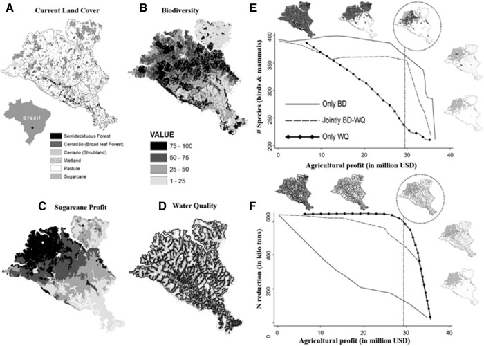
Spatial action maps showing potential for profitable agricultural expansion under various levels of compliance with environmental regulations in Brazilian Cerrado. (A) Current land cover and land use for the Ribeirão São Jerônimo study watershed in southeastern Brazil. Prioritization maps depicting the relativized marginal values for (B) biodiversity, (C) sugarcane profit, and (D) water quality in the watershed. Efficiency frontiers show marginal losses and tradeoffs between agricultural profit and biodiversity (only BD), water quality (only WQ), or both BD and WQ (joint BD‐WQ) for species (E) or water quality (F) returns. The circled maps illustrate optimal protection/restoration of 25% of native habitat that coincides with the Brazilian Forest Code's habitat threshold for the region. Maps were produced using economic and biophysical production function models. Additional details under the Agriculture Siting case in Table 2. Modified and reproduced with permission. ⁹⁰ , ¹³²

Spatial action maps can also be used to compare actions. For example, spatial action maps were combined with cost data associated with reforestation or avoided deforestation to show the potential of these two actions to mitigate atmospheric carbon across the tropics (Fig. 5A and B). The maps allow stakeholders to see which action has the most cost‐effective potential in a given place. For example, the Democratic Republic of Congo has much more potential for emission reductions through avoided deforestation than through reforestation (Fig. 5C, country label COD).

Figure 5.

Spatial action maps of potential atmospheric carbon reductions thought forest restoration or avoided deforestation in the tropics. At a carbon price of US$20 tCOe⁻¹ from 2020 to 2050, maps show potential removals from reforestation (A) and reduced emissions from avoided deforestation (B). Combining the maps allows a ranking of 77 countries based on their potential to reduce carbon emissions through both actions (C). Axes are log‐scale, blue data are for Latin America/Caribbean; orange data are for Africa; and green data are for Asia. The three‐letter country codes are from the UN trade statistics (https://unstats.un.org/unsd/tradekb/knowledgebase/country‐code). Additional details under the Tropical Carbon case in Table 2. Figure modified and reproduced with permission. ¹⁵²

As another example, in an analysis of where and how much urban street tree planting could reduce urban heat and air pollution, spatial action maps were combined with cost data to estimate how returns on investment could be optimized (Fig. 6).

Figure 6.

Return on investment (ROI) of urban street planting for particulate air pollution reduction in Washington, DC. Inputs to spatial action maps included land cover (A), forest cover (B), current particulate matter concentration (PM) (C), and population distribution (D). Spatial action maps were combined with cost data to estimate ROI for individual street segments (E), as well as for 1‐km grid cells (F). Additional details under the Urban Trees case in Table 2. Adapted and reproduced with permission. ¹²⁸

Spatial action mapping will be most useful when actors can implement actions on a subset of a large land‐ or seascape. This is often the case in conservation planning contexts where there is a mosaic of public and private lands or waters, and various stakeholders control actions in different places. Such mosaics set the stage for conservation actions to be one aspect of a larger, dynamic system, most of which the conservation decision maker does not control or cannot influence. Spatial action mapping can usefully place conservation actions in the context of other forces acting across the land‐ or seascape.

Alternatively, decision processes that address multiple uses across an entire land‐ or seascape are not best served by spatial action mapping. For example, some national land use planning or marine zoning processes have the potential to influence a range of uses across entire land or seascapes. Multiobjective scenario planning is better suited to these cases, as it provides a better framework for representing the interactions among simultaneous changes in drivers affecting whole land‐ or seascapes. ⁸⁸ , ⁹⁰

Engagement with key stakeholders is critical throughout the entire conservation planning process, ¹² , ¹⁰⁰ , ¹⁰¹ and the steps associated with spatial action mapping are no exception (Fig. 7). Planners, community leaders, traditional knowledge holders, activists, and many others can provide important input to spatial action mapping processes. A variety of strategies and extensive guidance are available for seeking stakeholder input, from key informant or focus group discussions to intentional choice experiments. ¹⁰²

Figure 7.

Sample stakeholder inputs to spatial action mapping processes. Spatial action maps are more likely to influence decisions when they are created in close collaboration with stakeholders throughout their development. Examples of relevant input that stakeholders can provide at each step are presented here. This is not an exhaustive list.

A main purpose of stakeholder engagement in spatial action mapping is to understand the decisions at hand, specify alternate possible actions, and ensure that spatial action mapping is codesigned as a useful tool for informing decision makers (Fig. 7). Decision‐making processes where spatial action mapping may add value include community visioning processes, planning for natural resource management, biodiversity strategic actions, endangered species management, infrastructure development and mitigation, subnational comprehensive plans (e.g., municipal or state), climate resilience and risk reduction, food or water security, corporate supply chains, local economic development, urban development, policy design, and behavior change or communication campaigns, among others. While some of these conservation approaches are not typically considered spatial (e.g., policies and communication plans), all do have impacts that may vary across space, so should and can be considered. For example, communication campaigns with different messaging or messengers are likely to reach different audiences who live in different places or change behaviors that affect different places. Understanding this variation in outcomes may help better design policies and campaigns. Engagement with decision makers in any such process is critical to understanding the decisions that will be made and whether spatial action mapping is relevant.

In addition to the decision makers who may act based on findings, other stakeholders across diverse skills and perspectives are critical to engage. Any representation of proposed interventions is likely to be strengthened through input from stakeholders who may have authority over relevant aspects of the larger system, ¹⁰³ strong opinions about the location or impact of actions being considered, or whose lives or livelihoods may be affected by the actions. Other important stakeholders may not be affected by the decision at hand, but may hold knowledge about the impacts of interest, the feasibility of actions being considered, or the probability of adoption. These stakeholders may include those making other decisions about the system that can hinder or amplify the actions being considered.

The methodology

Our framework assumes that spatial action mapping starts after the foundations of a conservation planning process have been established (Fig. 1A). These foundations typically include clarification of the decisions to be informed by the mapping, the scope (geographic, temporal, and strategic) for the mapping exercise, the environmental and human wellbeing goals, and candidate actions that could be taken to achieve the goals. ¹¹ , ¹² , ¹⁰⁴ For example, a spatial action map may be developed to evaluate which countries with savanna landscapes (the geographic scope) could make a substantial contribution to national greenhouse gas emissions reductions (the goal) through proactive early dry season burning (the action). ¹⁰⁵ Spatial action mapping builds on this foundational work.

We describe a framework for spatial action mapping that follows four steps that specify: (1) which action(s) is being taken, by whom, and to what ends; (2) how the system will behave if the action(s) is not taken; (3) where the action(s) is likely to take place, including feasibility and probability of implementation as designed; and (4) how much impact the action(s) will have considering the expected effectiveness of the action under specified socioecological conditions (Fig. 1B). Methods applied at each step can range in complexity, with varying data needs, analytical approaches, and capacity requirements (Table 1). We give a selection of examples that represent application of this approach to various types of actions, diverse geographies, and a range of spatial scales, using different levels of complexity for each step in the process (Table 2). The examples are not meant to demonstrate ideal spatial action maps, but rather to show a range of applications of the general framework under the varying constraints of conservation planning in practice.

Table 1.

Options for spatial action mapping methods

Step	Less Complex More Complex
Specify impacts	Impacts nominated and selected through ad hoc process	Impacts identified through logic models	Impacts identified through logic models, evidence evaluation
		Impacts narrowed through use of value tables with stakeholders
Create BAU Scenario	Basic assumptions (e.g., resource use expands where cost‐effective and legal)	Statistical projections based on historic patterns of change	Functional modeling (e.g., reflect human behavior, changing environmental conditions, etc.)
Create action scenario	Single value adjustment for probability of adoption	Continuous value adjustment for probability of adoption	Probability of adoption modeled based on multiple factors, including human preferences and local conditions
	Action represented as “present”	Action represented as basic changes in land use/land cover or other spatial variables	System changes in response to action depicted through complex modeling
Estimate benefits and losses	Overlay scenarios on current conditions, apply factor adjustments	Calculate changes based on literature coefficients	Calculate changes using process models, sometimes including dependencies, feedbacks, and interactions

note: The general steps of spatial action mapping can be completed using a wide range of methods that vary in complexity and associated time, capacity and resource requirements to complete. This table details a range of options for several steps of the process. These options are not exhaustive. Spatial action mapping may include creation of multiple BAU and/or action scenarios. BAU, business as usual.

Table 2.

Spatial action mapping cases

		Case
Title		Urban trees	Tropical carbon	Marine protection	Forest conservation	Energy siting	Invasives control	Agriculture siting
Application		Urban trees planting to reduce heat, air pollution	Reforestation and forest conservation to reduce greenhouse gas emissions	Debt swaps to fund marine protected areas	Natural habitat conservation to provide ecosystem services	Meet renewable energy commitments with minimal biodiversity impacts	Invasive species control to benefit water supplies	Expand agriculture, complying with environmental law
Spatial scale		Global	Global	Global	National	Subnational	Local	Local
Geography		Global	Global tropics	Global	Myanmar	Western USA	South Africa	Brazilian cerrado
Specify actors, actions, impacts	Action(s)	Tree planting	Forest conservation funded by carbon payments	Protection funded by government debt restructuring or debt forgiveness	Conservation of natural habitat (avoiding agricultural conversion)	Wind, solar, and geothermal energy infrastructure development with environmental conservation	Invasive plant removal	Sugarcane and cattle pasture expansion
		Natural regeneration						Natural habitat restoration
			Reforestation funded by carbon payments					Natural habitat protection
	Actor(s)	Municipal governments	Government staff, landowners, community members, and forestry companies	Private insurers, creditors, or development finance institites	National government	Utilities making power purchase decisions	Municipal authority	Private corporation
		Private landowners		National governments
	Decision maker(s)	Mayors	Government ministers, CEOs, landowners, and community leaders	Global nonprofit organization	National government	Utilities making power purchase decisions	Municipal authority	Private corporation
		Urban planners
	Impacts estimated (difference in…)	Particulate matter concentration near residents	Forested area	Human threats in marine systems	Drinking water sediment pollution	Renewable energy production	Water quantity	Species persistence probability (407 birds and 132 mammals)
		Summer air temperature near residents	Atmospheric carbon concentrations	Human threats in coral reefs areas	Sediment pollution upstream of dams	Cost of energy provision	Jobs created	Net profit from sugarcane and cattle ranching
					Dry season drinking water availability	Amount of sensitive land area impacted by energy development	Cost per cubic meter gained water supply	Water pollution (nitrogen, phosphorus, and sediment)
					Riverine flood risk to villages
BAU scenario	Basis for BAU scenario	Current tree cover	Expected agriculture expansion and carbon accumulation	Current conditions	Expected agriculture expansion and climate scenarios	Meet renewable energy targets, ignore environmental impacts	Expected invasive species expansion	Agriculture expansion with no Forest Code compliance
	Method used to create scenario	No BAU created	Dynamic‐recursive projection of annual forest loss/gain in 2020–2050, assuming no changes in agroecological, economic, and policy conditions	No BAU created	All natural habitat (2013–2014) converted to agriculture, combined with several existing downscaled climate models	Models applied to expand renewable energy infrastructure based on energy site suitability, but not environmental exclusions	Used existing scenarios	Converted current land uses to sugar cane or cattle ranch to maximize net profit
Action scenario	Feasibility: physical factors	Aridity index suitable Nonimpervious land cover	Continent and biome Elevation Distance from cities Current forest cover	Presence of high conservation value marine area	Presence of natural habitat	Environmental exclusion categories based on conservation values, land ownership, and protection status. Energy site potential factors, including energy potential, physical characteristics, hazards, and economic viability	Presence of dense invasive plants	Multiple biophysical, sociopolitical, and economic factors incorporated in models used to generate scenarios of optimal agriculture expansion
	Feasibility: sociopolitical factors	Population distribution	Protection status				Inside water source area
		Cost of tree planting
	Feasibility: economic factors	Vulnerable sites (schools and hospitals)	Carbon payment of USD20 or USD50/tCO2e greater than agriculture revenue and transaction costs	Debt to GDP ratio 60% or higher
	Method used for probability of adoption	Assumed 100% when feasibility conditions met	Assumed 100% when feasibility conditions met	Assumed 100% when feasibility conditions met	Assumed 100% when feasibility conditions met	Assumed 100% when feasibility conditions met	Assumed 100% when feasibility conditions met	Varying levels of Forest Code compliance, farm or landscape scale compliance
	Method used to create scenario	Action represented as marginal increase in tree cover in each 1‐km grid cell	Iterative land use and land cover change based on carbon payments. Reforestation created natural or plantations; conservation retained existing forest cover	Action represented as “present”	Current (2013–2014) land use/land cover map to represent no further natural vegetation loss, combined with downscaled climate scenarios	Models applied to expand renewable energy infrastructure based on energy site suitability, and three different levels of environmental exclusions	Used existing scenarios	Iterative optimization of land use configurations based on different levels of Forest Code compliance, scale of compliance, preferences for each outcome
Estimate benefits and losses	Methods used	Moderately complex: models of air pollution, temperature, and health significance based on literature coefficients	Moderately complex: production function models used to estimate above and below‐ground carbon and atmospheric CO2 removals	Less complex: area of EEZ (total or area containing coral habitat) adjusted by abatable and unabatable threat scores	Moderately complex: InVEST models for all ecosystem service estimates, largely rely on production functions models based on literature coefficients	Moderately complex: linear programming model RESOLVE used to create supply curves. Less complex overlay approach for environmental impacts	More complex: Water Resources Yield Model, WR2005 and ResSim models for water quantity	Moderately complex: economic, ecological, and biophysical production function models
Source		128	152	108	115	106	109	90, 132

note: Cases provide specific examples of how spatial action mapping has been done at local to global scales and for a wide range of conservation actions. Each case combined methods based on stakeholder interests, resource, and data availability and other factors. Cases show combinations of different levels of complexity in the methods used across various steps of the process. Full details of methods for each case can be found in their source publications.

Specify actors, actions, and impacts

We recommend starting a spatial action mapping process by clearly describing the actions to be assessed, the actors assumed to be taking those actions, and the impacts of the actions that will be estimated. In short, this step clarifies what, by whom, and to what ends. Stakeholder input is critical in this step, and alignment with the focal decision makers and implementers on these aspects is essential (Fig. 7).

While goals and possible actions may already be identified through earlier steps in the conservation planning process (Fig. 1A), decisions may need to be specified further to support spatial action mapping. For example, a team that has identified protection as a possible conservation action may not have been specific about which types of protection are to be included (e.g., private versus public protected areas: strict nature reserve, wilderness area, and national monument). As these types of protection are relevant under different conditions and may result in different biodiversity and human wellbeing outcomes, further specification is needed before possible areas for each type of protection can be mapped. Participants in the Energy Siting case (Table 2) went beyond generic ideas of protection by describing four potential actions that applied increasingly stringent levels of environmental protection, each of which led to a different map of potential areas. ¹⁰⁶ Alignment on specific actions early in the mapping process will ensure that stakeholders have the same expectations and will streamline later steps. ¹⁰⁷

At this stage, it is also important to specify which actors are to be reflected in the analysis. This is not the same as identifying relevant stakeholders (see section above), but rather, which subset of stakeholders’ actions will be represented in the scenarios created. This is often an aspect of conservation prioritization that is implied rather than explicitly stated. Specifying the actor(s) represented in the mapping will help inform later assumptions and inputs regarding feasibility of the action(s) and probability of success. For example, different actors may have potential to drive actions in different geographic areas, under differing conditions, with differing resources and capacities. A spatial action map of natural reserve establishment will look different when the actor is a global land trust organization than when the actor is a specific national government or a particular coalition of Indigenous communities. The actor(s) and decision maker(s) may or may not be the same. For example, in the Marine Protection case (Table 2), the decision maker using the mapping analysis was a global nonprofit organization, but the actors included were national governments. ¹⁰⁸ By contrast, the Cape Town municipality was both the actor and decision maker in the Invasives Control case. ¹⁰⁹

Finally, it is important to gain agreement and clarity on which impacts (positive and negative) will be estimated. Relevant impacts may have been identified in earlier conservation planning steps focused on setting goals. If not already chosen, likely impacts can be identified using logic models, which describe causal pathways from actions to environmental and human impacts. ¹² , ¹¹⁰ , ¹¹¹ They can also reveal possible negative unintended consequences, which may be chosen as part of the mapping exercise to identify areas where tradeoffs can be minimized. ⁹⁰ , ⁹¹ , ⁹³ We suggest considering impacts that (1) relate to the stated conservation goals; (2) are likely to result from the proposed actions undertaken by the specified actors; (3) are of greatest interest to key stakeholders; (4) are likely to vary spatially; and (5) can be quantitatively estimated in a spatially explicit manner.

Actions can cause many benefits and losses, so there may be a need to narrow the list based on stakeholder interests. This is often done implicitly, as is true for all seven cases we include. However, as different stakeholders are likely to have different interests, we recommend making this process explicit. Simple options may include facilitating stakeholder dialogues, while more complex options include elicitation of weights within a structured, participatory decision‐making process. ¹¹²

Data, model, and capacity limitations may make it impossible to estimate changes in some impacts that are of interest to stakeholders. For example, the activities mapped in the Urban Trees case can reduce particulate matter and heat‐related mortality (Fig. 6). The same actions also likely lead to reduced disease in urban residents. However, these additional health impacts were not modeled due to the much smaller number of available published exposure‐response functions for many morbidity effects of particulate matter and heat, and the large data collection effort such modeling would have required. Iteration between impact selection and analytical design will help arrive at a set of impacts that are logically linked to selected actions, of interest to at least one stakeholder, and feasible to estimate.

Calculation overview

A robust spatial action mapping process moves beyond asset and threat assessments by using basic scenario analysis. The approach builds a spatially explicit (mapped) view of potential impact for each spatial unit (x = 1, 2, ….X) on a land or seascape, where a unit can be any user‐defined option, including a grid cell, a hexagon, a polygon, and so on. Conditions under a BAU future are compared with conditions in a future with the chosen action(s) implemented (Fig. 1B). Potential impact (I) of a chosen action (a) is calculated as:

$$I_a=\sum _{x=1}^{X}f(Q_{Ax},F_{ax},P_{ax},D_{ax})-Q_{BAUx},$$ (1)

where the status of the chosen impact under the action scenario (A) is a function of the quantity of expected impact I generated by perfect adoption of the action (a) under the set of conditions in parcel x under the action scenario (Q_Ax ), adjusted for the feasibility of action a occurring in parcel x (F_ax ), the probability that action a will be adopted in parcel x if it is feasible (P_ax ), and the likelihood that action a is implemented as designed in parcel x (D_ax ). Q_BAUx is the amount of the chosen impact I generated in parcel x under the BAU scenario. A spatial action mapping analysis may consider multiple impacts from a given action, and may also consider multiple actions, each with their own associated impacts.

Each calculation is discussed further in the following sections. As the equations we provide represent general functions, their form and expression will be different in each application, with planners deciding if and how to express each variable within the constraints of their analysis. We provide qualitative descriptions of seven different applications of this framework (Table 2). Original source papers for the examples give further detail and quantitative expressions of the calculations.

Create BAU scenario

BAU scenarios are commonly used in policy evaluation to assess how outcomes in a scenario with the policy or program under evaluation differ from those in a scenario without the policy or program. ¹¹³ The purpose of a BAU scenario is to depict what would happen absent the policy or program (i.e., the world without the policy); thus, the BAU scenario should include expected changes in key variables that affect the outcomes of interest, including relevant policies, population, economic activity, and technology. ¹¹⁴ In the context of spatial action mapping, the BAU scenario is meant to depict the system at a particular time point in the future as it will be if the conservation action being explored is not taken.

A BAU scenario is distinct from a current baseline or historic reference condition, which are sometimes used in other types of conservation analyses. Using these types of scenarios as a BAU scenario in spatial action mapping could lead to over or underestimation of impact, result in underestimated additionality of actions (by directing actions to places that may be under high threat today, but lower threat in the future), or result in missed opportunities (by underrepresenting a threat in an area where a risk is expected to increase in the near future). In general, the most informative comparison in a spatial action mapping analysis will come from the use of a BAU scenario that represents changes in the future without the candidate action. For example, the Forest Conservation case created BAU scenarios that depicted expected agricultural expansion without additional forest conservation and included a range of expected climate conditions ¹¹⁵ (Table 2; the Forest Conservation case). In some cases, such as actions to mitigate climate change, extensive debates have established alternative means of setting BAU scenario conditions. ¹¹⁶

The BAU scenario is informed by the proposed action(s) and what it is expected to change. For example, in the Invasives Control case (Table 2), the proposed action is the removal of invasive alien plant species above and beyond rates achieved by BAU control efforts, so the BAU scenario was designed to depict vegetation cover (of native and nonnative species) without additional invasive species removal actions. Use of a current map of invasive species distribution as the BAU scenario in this case would misrepresent the conservation impact because the focal invasive species are expanding rapidly, and this expansion would not be captured.

There are multiple approaches to developing spatially explicit BAU scenarios (Table 1). One option is to apply basic assumptions to determine how conditions will change. For example, when exploring actions that will reduce or change the location of resource extraction, one could assume that planned new development will happen in places where it is legal and cost‐effective. This approach has been used to create BAU scenarios for growth in energy infrastructure, agriculture, fisheries, and mining. ¹¹⁷ , ¹¹⁸ , ¹¹⁹

Alternatively, statistical models can be developed based on past patterns and applied to project those patterns forward into the future. ¹²⁰ , ¹²¹ This is appropriate when no major changes in the size or effect of drivers of change are expected over the projected time frame. This approach was used in the Tropical Carbon case, where trends in drivers between 2000 and 2010 were used to project the same drivers into 2020–2050 (Table 2). A similar approach was used at a smaller scale in Indonesia to extend recent patterns of illegal forest encroachment as a BAU scenario for enforcement actions. ¹²²

Another option for creating a BAU scenario is to model future processes that are expected to change drivers of interest (e.g., climate change, policy, and cultural shifts). Options for this type of approach include system models, cellular automata models, multiagent system models, among others. There are many cases of using this approach to estimate land use and land cover changes into the future. Examples include use of a cellular automota‐Markov chain model for Dedza district, Mali, ¹²³ and development of a generalized agent‐based model for larger scale applications. ¹²⁴

In some instances, there is no historic experience with the major drivers of interest. In these cases, it may be most appropriate to use multiple BAU scenarios that represent a range of possible conditions without the proposed action, and to characterize uncertainty around the future state. Climate change is a driver often treated in this way, as patterns in key environmental drivers are already varying from observed, historic patterns. The authors of the Forest Conservation case included multiple climate futures in combination with both their BAU and action scenarios (Fig. 3 and Table 2, the Forest Conservation case).

In many cases, existing analyses may be used as BAU scenarios, or as inputs to creating them. Government, research, and/or industry groups regularly create scenarios or spatial plans of expected future changes in many possible aspects of a BAU scenario (e.g., energy, agriculture, transportation, infrastructure development, and climate change). These may take the form of national energy plans, agricultural zoning plans, infrastructure development proposals, global climate change scenarios, and so on. Maps of biodiversity threats or human conversion pressure ¹²⁵ , ¹²⁶ may also serve as useful inputs to the creation of BAU scenarios. One caution in considering threat maps is that many capture current, rather than future, threat levels, and the drawbacks of using present or historic conditions have been discussed above.

Create action scenario

The action scenario depicts a future where the proposed action is implemented. Creation of the action scenario captures key changes that the action will cause, against the backdrop of other expected changes that the action does not affect. For example, in a case exploring the impacts of switching from high to low water use crops, the action scenario might represent the intended change in land use in the context of climate change and expected changes in other water uses.

The action scenario incorporates the action's feasibility (F_ax ) and likelihood that it will be implemented to design (D_ax ) (see Eq. 1). Feasibility is often influenced by a suite of physical, social, institutional, and economic conditions related to both the action and the actors undertaking it. The action scenario aims to represent the influence of these factors on adoption of the action. Some feasibility factors have clear thresholds and so are amenable to binary representation. For example, a debt swap is an action that can be taken to enable a national government to take some conservation action, such as establishing new protected areas. In the Marine Protection case (Table 2), the condition of the debt available for restructuring was treated as a binary feasibility factor, where swaps were considered feasible in any country with a debt to GDP ratio of 60% or higher. ¹⁰⁸ The specific factors determining feasibility will vary by action, actor, and case, and stakeholder engagement is critical for informing this step (Fig. 7).

The action scenario should also reflect the probability of adoption (P_ax ), defined as the likelihood that the action will be adopted in a place where it is feasible. In many conservation planning exercises, it is assumed that an action will be adopted in all the places where it could have impact. In our diverse examples of spatial action mapping, all but one assumes 100% probability of adoption in places that meet the feasibility criteria (Table 2; the Action Scenario: method used for probability of adoption). These cases assumed 100% adoption to represent the full potential of the actions explored, but complete adoption is uncommon. For example, economic subsidies have incentivized the use of cover crops in U.S. row crop systems for many years, but actual adoption remains around 3.9%. ¹²⁷

There are several options for adjusting the action scenario to reflect the probability of adoption (Table 1). A simple approach is to use a single estimate to reduce the feasible area in the action scenario. For example, the data on cover crop adoption could be used to reduce expected adoption in any new programs to ∼4% of prospective adopters. A more complex approach to projecting adoption may be possible if conditions for adoption are understood and relevant data are available. Data on such conditions may be used to select subsets of areas considered feasible for the action (e.g., ruling places “in” or “out”). For example, community‐based fishery closures may have a 45% adoption rate where they are feasible and be most likely to be adopted in communities with an identified community leader. This information could be used to select 45% of feasible areas, preferencing selection of communities with identified community leadership. A continuous variable could be used in a similar way, selecting areas with diminishing value until the target level of adoption is met. When multiple factors or social learning are known to influence the rate of adoption, a yet more sophisticated approach could use an estimation function, including relevant factors, to estimate variation of adoption across space.

Once feasible locations for the action and actor have been determined and adjusted for probability of adoption, choices must be made about what variables in the action scenario to change to reflect adoption. The approach used here is often dictated by the analyses planned to estimate the impacts of interest in the next step. A simple approach is to identify the action as present in those areas where it is determined to be feasible and likely to be adopted. This approach is appropriate if impacts are going to be estimated through factor application or a similarly simple method, such as those applied in the Marine Protection case (Table 2). If impacts are going to be estimated functionally based on conditions in a given parcel, then the action scenario should reflect any relevant changes the action is expected to cause in the factors included in the functional equation. For example, if an impact will be estimated as a function of a single spatial data layer, such as land use/land cover, or vegetation density, the action scenario needs to reflect the action as an altered land use/land cover type, or adjusted vegetation density. This approach was used in the Urban Trees case (Table 2), where the action scenario increased the percent cover of urban street trees in 1 km grid cells, and the decrease in air pollution and heat stress impacts on the residents of this grid cell were estimated using biophysical models. ¹²⁸ There may need to be iteration between steps within the spatial action mapping process (Fig. 1B) to ensure that factors used in estimating impact are adjusted appropriately in the action scenario.

An additional variable, D_a , can be introduced to account for the reality that conservation actions are not always implemented as designed. This variable is defined as the likelihood that the action a is fully implemented as designed. Many spatial conservation planning analyses assume that a given action will always be implemented as designed and return an ideal conservation outcome (e.g., removed extinction risk for all species; complete restoration of a degraded system; and perfectly sustainable resource extraction). However, implementation of an action can be incomplete, reducing its impact. Often, partial implementation results from weak enforcement of actions, such as poor enforcement of activity limitations (e.g., stopping illegal logging or fishing within national protected areas). ¹²⁹ , ¹³⁰ , ¹³¹ Such partial adoption was explored in the Agriculture Siting case, where scenarios were created to represent different levels of compliance with existing environmental regulations in Brazil. This case also considered the differences in profit and environmental impacts when actions were implemented to ideal design (by optimizing profit and environmental gains as dual objectives) versus suboptimal design (by reducing private costs then accounting for environmental damages) ⁹⁰ , ¹³² (Table 2; the Agriculture Siting case).

This factor can also be estimated through a variety of methods (Table 1). In a simple approach, a single adjustment can be applied to all areas where adoption is expected. For example, enforcement of protected areas is known to be low in countries with government corruption. ¹³³ Consider an analysis of the potential for protected areas to impact threatened and endangered bird populations and tourism revenue in Kenya, Tanzania, the Democratic Republic of the Congo, Namibia, and Botswana. Each of these countries experiences corruption according to the Corruption Perceptions Index (CPI), ¹³⁴ so a single value could be applied across these countries to diminish the likely impact of protection given that corruption is likely to weaken implementation. However, since the CPI is a continuous index, a more complex approach could be taken by using each country's index value as a factor to reduce likelihood of implementation to design. Many factors can alter the likelihood of implementation to design, including capacity or data limitations, biased data, incomplete information, budget limitations that lead to incomplete or altered implementation, infrastructure constraints that limit access or supplies, weak social networks, or stakeholder biases, among others. ¹³⁰ Stakeholder engagement can help reveal relevant factors for the system of interest, prioritize the ones to include in the analysis, and inform how constraints are reflected.

Estimate benefits and losses for nature and people

In the final step of spatial action mapping, focal impacts are evaluated under the BAU and action scenarios, and the difference between scenarios is calculated to estimate benefits and losses from the action (Fig. 1B). This step addresses estimation of impact under BAU (Q_BAU ), and the remaining elements of estimating impact under the action scenario (Q_A ). The quantity of an impact of interest (e.g., species extinction risk, greenhouse gas emissions, or income from nature‐based livelihoods) varies on the basis of some set of factors in the system and an action creates impact by altering one or more of those factors. As such, a consistent approach can be used to estimate the quantity of impact under the BAU and action scenarios, and the difference in conditions within the scenarios will allow estimation of gains and losses caused by the action (see Eq. 1). As with other steps, a range of approaches can be used to estimate these values. ¹³⁵ We do not review all plausible approaches here, but rather identify several options along a spectrum of complexity (Table 1).

In a simple approach, one may be able to use existing estimates of the impact under BAU (Q_BAU ), and derive impact under the action scenario by applying a single factor adjustment to BAU levels of the impact as follows:

$$Q_{Ax}={\alpha }_a{Q}_{BAUx,}$$

where α _a is an adjustment factor indicating the expected effect of action a on impact Q in parcel x. For example, many conservation planning analyses take this approach by implicitly applying α_a = 1 in all places where an action is assumed to be taken (e.g., assuming the impact of a protection action is to keep all existing species and habitats in their current status). It is unlikely that impacts will be the same everywhere, but this simplifying assumption may be necessary in the absence of information about how impacts vary, or when the analysis faces other constraints. This type of approach was used in the Marine Protection case, where debt swaps were assumed to drive marine protected area establishment that would yield perfect removal of all threats that can be abated by that action (e.g., overfishing) ¹⁰⁸ (Table 2; the Marine Protection case).

The next tier of complexity would involve estimating Q_BAU and Q_A as a function of several coefficients derived from the literature and applied to relevant data describing conditions known to influence impact:

$$Q_x=f({\beta }_1{Y}_{1x},{\beta }_2{Y}_{2x},{\beta }_3{Y}_{3x}\dots \dots \dots {\beta }_n{Y}_{nx}),$$

where β₁ …..${\beta }_n$ are coefficients from the literature corresponding to $Y_{1x}$ ….. $Y_{nx}$ which are factors known to affect the impact of interest. In some cases, the equations used to estimate Q_BAU and Q_A may be identical, with variation in impact being driven by variation in the values of the factors ($Y_{1x}$ ….. $Y_{nx}$) between the scenarios. If new factors are introduced through the action scenario, then different functions may be needed to represent these new factors. Conceptual models (also called logic models, result chains, theories of change, and influence diagrams) can be useful starting points for informing this kind of factor‐based estimation model. Such logic models are commonly created in other steps of the conservation planning process and reference examples exist for some conservation actions. ⁴²

This factor‐based approach was used in the Agriculture Siting case to investigate the potential for targeted land‐use planning to achieve both commodity production and environmental goals in the Brazilian Cerrado ⁹⁰ (Fig. 4 and Table 2, the Agriculture Siting case). Specifically, spatial optimization techniques were used to map marginal values across a watershed to determine where the next unit of habitat clearing versus habitat restoration or protection would be most costly or beneficial in terms of agricultural profit (estimated for sugarcane production and cattle ranching), biodiversity (estimated as bird and mammal species persistence probability), and water quality (estimated as levels of nitrogen, phosphorous, and sediment retention). Efficiency frontiers that plotted agricultural profit against biodiversity and/or water quality were used to assess the marginal loss of those services per unit gained in profit and to detect potential land‐use thresholds at different adoption scales (farm versus watershed scales) and compliance levels under Brazil's Forest Code. This approach allowed decision makers to see which configuration of agricultural growing areas, habitat protection, and habitat restoration areas best met their multiple objectives.

The factor‐based estimation approach is also used for ecosystem service and biodiversity impacts in the open‐source software tool InVEST ¹³⁶ and its sister tools RIOS, ¹³⁷ OPAL, ¹³⁸ MESH, ¹³⁹ and ROOT. ¹⁴⁰ InVEST has been used in many environmental decision‐making contexts, including the Forest Conservation case (Table 2). In this case, sediment retention, dry season baseflows, and flood risk reduction benefits provided by forested areas were estimated using a production function approach. ¹¹⁵ Resultant maps (Fig. 3) show variation in areas with potential to secure the benefits of interest, with the most important areas largely falling outside the country's current protected area network but remaining highly consistent across the range of climate scenarios considered.

Further complexity could be incorporated into the estimation of Q_BAU and Q_A using process models that depict the underlying functions of the system that interact to produce the impact of interest. Process models reflect the underlying biophysical, social, and economic drivers of change in the system, and potentially include interdependencies among these processes and/or feedbacks within the system. Such processes relevant to estimating conservation impacts would include climate dynamics, environmental (e.g., migration), and social (e.g., trade) teleconnections across spatial scales, dynamic processes, such as biogeochemical processes, human learning, and behavior change, and other relevant processes. Examples include Bayesian network ¹⁴¹ , ¹⁴² and integrated assessment models (GCAM; ¹⁴³ GLOBIOM, MIRAGE‐BioF; ¹⁴⁴ and FASOM ¹⁴⁵ ). These models have the advantage of reflecting more of the underlying dynamics and nonlinearities in complex systems and they are likely to provide the potential to estimate some subset of multiple impacts through an integrated set of assumptions and data. However, they generally have extensive data requirements and are inevitably more constrained by available data, capacity, and resources to apply them in new settings.

Frontiers in spatial action mapping

Many conservation planning analyses fall short of their potential utility because they do not account for how the key actions, questions, and impacts of interest to relevant decision makers and stakeholders vary spatially. We have outlined an approach that explicitly considers which conservation actions are being taken by whom and uses basic scenario analysis to estimate conservation impact compared with a future without the action. This approach embeds several advances in spatial mapping (e.g., mapping feasible areas for nonprotection actions, accounting for variation in adoption and implementation, replacing static maps with estimates of impact, and including multiple ecological and socioeconomic impacts) into standard conservation planning frameworks. When combined with ROI assessments that represent variation in costs, spatial action mapping can dramatically increase the benefits of prioritizing conservation actions.

However, this approach faces several limitations in practice. Through this methodology, we make three things explicit that are usually implicit in spatial conservation prioritization: variation in the feasibility of conservation actions, variation in actual adoption of conservation actions, and variation in an action's effectiveness. While introducing variables to describe these factors provides a way to directly address the variation we know exists, doing so reveals uncertainty when actual relationships are not understood or data to describe them are poor. Major data gaps do exist for some of these variables. Improvements in conservation impact evaluations and a broad range of data sources are needed to fully enable the application of the spatial action mapping approach. Impact evaluation transformed the medical sciences when it emerged in the 1700s, in the form of randomized control trials. ¹⁴⁶ While impact evaluation methods have proliferated across other fields, they have only more recently become influential in the design of development and conservation efforts. ¹⁴⁷ Growth in impact evaluations would provide valuable fodder for spatial action mapping.

In addition, the factors that determine the feasibility of an action, and objective reporting on how often actions are implemented as designed are incredibly limited. In turn, there is a clear need to better understand how estimates of feasibility are linked to performance of conservation interventions. There are also often mismatches in spatial and/or temporal resolution of data inputs for estimating multiple, diverse impacts. For example, the Urban Trees case had access to high‐resolution land cover data for estimating forest cover and projecting its change, but particulate air pollution data for the same region were very coarse (Fig. 6).

Conservation actions also take place in the context of complex land and seascapes where many individuals (human and other species) are interacting across space and through time; and while these complex interactions are often difficult to realistically account for, they are essential to strive to better understand as they can lead to nonlinearities in impact, probability of success, and conservation costs. ¹⁴⁸ , ¹⁴⁹ As previously mentioned, approaches for addressing interactions in spatial action mapping should be more regularly employed, whether through simple (e.g., enlarging planning units to reduce influence of small‐scale interactions), moderate (e.g., running multiple plan scenarios to reveal influence of interactions on plan outcomes), or more complex (e.g., building complex dependencies into models that estimate impacts) approaches. Additional advances are needed to allow consideration of changes in conditions, likely outcomes, and the relevance or social value of such outcomes over time. ¹⁵⁰ , ¹⁵¹ More fully incorporating temporal variation would allow decision makers to explore where, how, and when to act, likely introducing additional efficiencies and improving conservation outcomes.

Given these known limitations and the uncertainties they introduce, it is critical to engage decision makers and relevant stakeholders early in spatial action mapping processes to understand how the uncertainties introduced may influence the decision at hand, and how these uncertainties may be explored and expressed in ways that can inform the decision (Fig. 7). It is useful to understand the decision maker's level of risk tolerance, as uncertainty that may be deemed scientifically interesting may be small (or large) relative to the decision maker's tolerance. There may be aspects of uncertainty introduced by the assumptions or data used that are not relevant to the decision, or that are unlikely to alter the decision. Understanding these aspects will help narrow in on the most critical types of uncertainty to explore and may offer insights into how that uncertainty can be most usefully expressed. When uncertainties are large and relevant to the decision process, mapping may need to be directed to alternative actions supported by clearer evidence or more sufficient data, or mapping may be paused while expert elicitation techniques or additional data collection or experimentation are done to allow reduction of uncertainties and distinction of options.

While limitations abound, methods and data are sufficiently advanced to support a spatial action mapping approach. The diversity of case examples included here and extending throughout the literature make clear what is possible. The alternatives—assuming that protection will be the conservation action taken and basing spatial conservation planning on threat and asset snapshots—are misaligned with modern conservation decision making. These practices should be phased out.

Competing interests

The authors declare no competing interests.

References

- 1. Millennium Ecosystem Assessment . 2005. Ecosystems and Human Well‐Being: Synthesis. Island Press. [Google Scholar]
- 2. IPBES . 2019. Global assessment report on biodiversity and ecosystem services of the intergovernmental science‐policy platform on biodiversity and ecosystem services. Bonn, Germany: IPBES Secretariat. [Google Scholar]
- 3. Soulé, M.E. & Simberloff D.. 1986. What do genetics and ecology tell us about the design of nature reserves? Biol. Conserv. 35: 19–40. [Google Scholar]
- 4. Secretariat of the Convention on Biological Diversity . 2010. Global Biodiversity Outlook 3 . Montreal. [Google Scholar]
- 5. McCarthy, D.P. , Donald P.F., Scharlemann J.P., et al. 2012. Financial costs of meeting global biodiversity conservation targets: current spending and unmet needs. Science 338: 946–949. [DOI] [PubMed] [Google Scholar]
- 6. Waldron, A. , Mooers A.O., Miller D.C., et al. 2013. Targeting global conservation funding to limit immediate biodiversity declines. Proc. Natl. Acad. Sci. USA 110: 12144–12148. [DOI] [PMC free article] [PubMed] [Google Scholar]
- 7. Possingham, H.P. , Bode M. & Klein C.J.. 2015. Optimal conservation outcomes require both restoration and protection. PLoS Biol. 13: e1002052. [DOI] [PMC free article] [PubMed] [Google Scholar]
- 8. Campos, F.S. , Lourenço‐de‐Moraes R., Llorente G.A. & Solé M.. 2017. Cost‐effective conservation of amphibian ecology and evolution. Sci. Adv. 3: e1602929. [DOI] [PMC free article] [PubMed] [Google Scholar]
- 9. Johnson, J.A. , Jones S.K., Wood S.L., et al. 2019. Mapping ecosystem services to human well‐being: a toolkit to support integrated landscape management for the SDGs. Ecol. Appl. 29: e01985. [DOI] [PubMed] [Google Scholar]
- 10. Strassburg, B.B.N. , Beyer H.L., Crouzeilles R., et al. 2019. Strategic approaches to restoring ecosystems can triple conservation gains and halve costs. Nat. Ecol. Evol. 3: 62–70. [DOI] [PubMed] [Google Scholar]
- 11. Schwartz, M.W. , Cook C.N., Pressey R.L., et al. 2018. Decision support frameworks and tools for conservation. Conserv. Lett. 11: e12385. [Google Scholar]
- 12. Fargione, J. , Tallis H., Morrison S., et al. 2016. Conservation by design 2.0 guidance document, version 1. The Nature Conservancy, Arlington. [Google Scholar]
- 13. Brooks, T.M. , Mittermeier R.A., da Fonseca G.A., et al. 2006. Global biodiversity conservation priorities. Science 313: 58–61. [DOI] [PubMed] [Google Scholar]
- 14. Game, E.T. , Kareiva P. & Possingham H.P.. 2013. Six common mistakes in conservation priority setting. Conserv. Biol. 27: 480–485. [DOI] [PMC free article] [PubMed] [Google Scholar]
- 15. Margules, C.R. & Pressey R.L.. 2000. Systematic conservation planning. Nature 405: 243. [DOI] [PubMed] [Google Scholar]
- 16. Groves, C. 2003. Drafting A Conservation Blueprint: A Practitioner's Guide to Planning for Biodiversity. Island Press. [Google Scholar]
- 17. The Nature Conservancy. 2006. Conservation by design, a strategic framework for mission success. Arlington, VA. [Google Scholar]
- 18. Foley, M.M. , Halpern B.S., Micheli F., et al. 2010. Guiding ecological principles for marine spatial planning. Mar. Pol. 34: 955–966. [Google Scholar]
- 19. Kingsford, R.T. & Biggs H.C.. 2012. Strategic adaptive management guidelines for effective conservation of freshwater ecosystems in and around protected areas of the world . IUCN WCPA Freshwater Taskforce, Australian Wetlands and Rivers Centre, Sydney. [Google Scholar]
- 20. Sayer, J. , Sunderland T., Ghazoul J., et al. 2013. Ten principles for a landscape approach to reconciling agriculture, conservation, and other competing land uses. Proc. Natl. Acad. Sci. USA 110: 8349–8356. [DOI] [PMC free article] [PubMed] [Google Scholar]
- 21. Sayer, J.A. , Margules C., Boedhihartono A.K., et al. 2017. Measuring the effectiveness of landscape approaches to conservation and development. Sustain. Sci. 12: 465–476. [Google Scholar]
- 22. Kremen, C. & Merenlender A.M.. 2018. Landscapes that work for biodiversity and people. Science 362: eaau6020. [DOI] [PubMed] [Google Scholar]
- 23. Porter‐Bolland, L. , Ellis E.A., Guariguata M.R., et al. 2012. Community managed forests and forest protected areas: an assessment of their conservation effectiveness across the tropics. For. Ecol. Man. 268: 6–17. [Google Scholar]
- 24. Daily, G.C. , Ceballos G., Pacheco J., et al. 2003. Countryside biogeography of neotropical mammals: conservation opportunities in agricultural landscapes of Costa Rica. Conserv. Biol. 17: 1814–1826. [Google Scholar]
- 25. De Beenhouwer, M. , Aerts R. & Honnay O.. 2013. A global meta‐analysis of the biodiversity and ecosystem service benefits of coffee and cacao agroforestry. Agric. Ecosys. Env. 175: 1–7. [Google Scholar]
- 26. Mendenhall, C.D. , Frishkoff L.O., Santos‐Barrera G., et al. 2014. Countryside biogeography of neotropical reptiles and amphibians. Ecology 95: 856–870. [DOI] [PubMed] [Google Scholar]
- 27. Shyamsundar, P. & Ghate R.. 2014. Rights, rewards, and resources: lessons from community forestry in South Asia. Rev. Environ. Ecol. Pol. 8: 80–102. [Google Scholar]
- 28. Torralba, M. , Fagerholm N., Burgess P.J., et al. 2016. Do European agroforestry systems enhance biodiversity and ecosystem services? A meta‐analysis. Agric. Ecosys. Env. 230: 150–161. [Google Scholar]
- 29. Beninde, J. , Veith M. & Hochkirch A.. 2015. Biodiversity in cities needs space: a meta‐analysis of factors determining intra‐urban biodiversity variation. Ecol. Lett. 18: 581–592. [DOI] [PubMed] [Google Scholar]
- 30. Barrow, E. & Murphree M.. 2001. Community conservation from concept to practice: a practical framework. In African Wildlife and Livelihoods: The Promise and Performance of Community Conservation. Hulme D. & Murphree M., Eds.: 24–37. Portsmouth, NH: Heinemann. [Google Scholar]
- 31. Berkes, F. 2007. Community‐based conservation in a globalized world. Proc. Natl. Acad. Sci. USA 104: 15188–15193. [DOI] [PMC free article] [PubMed] [Google Scholar]
- 32. Kiesecker, J.M. & Naugle D.E.. 2017. Energy Sprawl Solutions: Balancing Global Development and Conservation. Washington, DC: Island Press. [Google Scholar]
- 33. Robinson, B.E. , Masuda Y.J., Kelly A., et al. 2018. Incorporating land tenure security into conservation. Conserv. Lett. 11: e12383. [Google Scholar]
- 34. Duchelle, A.E. , Cromberg M., Gebara M.F., et al. 2014. Linking forest tenure reform, environmental compliance, and incentives: lessons from REDD+ initiatives in the Brazilian Amazon. World Dev. 55: 53–67. [Google Scholar]
- 35. Kidd, L.R. , Garrard G.E., Bekessy S.A., et al. 2019. Messaging matters: a systematic review of the conservation messaging literature. Biol. Conserv. 236: 92–99. [Google Scholar]
- 36. Ginn, W. 2020. Valuing Nature. A Handbook for Impact Investing. Washington, DC: Island Press. [Google Scholar]
- 37. Reguero, B.G. , Beck M.W., Schmid D., et al. 2020. Financing coastal resilience by combining nature‐based risk reduction with insurance. Ecol. Econ. 169: 106487. [Google Scholar]
- 38. Soto‐Montes‐de‐Oca, G. , Bark R. & González‐Arellano S.. 2020. Incorporating the insurance value of peri‐urban ecosystem services into natural hazard policies and insurance products: insights from Mexico. Ecol. Econ. 169: 106510. [Google Scholar]
- 39. Reilly, W.K. 2006. Using international finance to further conservation: the first 15 years of debt‐for‐nature swaps. In Sovereign Debt at the Crossroads: Challenges and Proposals for Resolving the Third World Debt Crisis , pp. 197–214.
- 40. Silver, J.J. & Campbell L.M.. 2018. Conservation, development and the blue frontier: the Republic of Seychelles’ debt restructuring for marine conservation and climate adaptation program. Int. Soc. Sci. J. 68: 241–256. [Google Scholar]
- 41. Puri, J. , Nath M., Bhatia R. & Glew L.. 2016. Examining the evidence base for forest conservation interventions. International Initiative for Impact Evaluation (3ie). Evidence Gap Map Report.
- 42. Conservation Actions and Measures Library. Accessed April 7, 2021. https://www.miradishare.org/ux/program/cmp‐conservationaction?nav1=caml‐projects.
- 43. Conservation evidence. Accessed April 7, 2021.. https://www.conservationevidence.com/Accessed.
- 44. Collaboration for environmental evidence. Accessed April 7, 2021. https://environmentalevidence.org/.
- 45. Rissman, A.R. , Comendant T., Kareiva P., et al. 2007. Private use and conservation protection on conservation easements. Conserv. Biol. 21: 709–718. [DOI] [PubMed] [Google Scholar]
- 46. Wilson, E.O. & Willis E.O.. 1975. Applied biogeography. Ecol. Evol. Commun. 260: 522–534. [Google Scholar]
- 47. Brockington, D. 2002. Fortress Conservation: the Preservation of the Mkomazi Game Reserve. Tanzania, Oxford, UK: James Currey Ltd. [Google Scholar]
- 48. Simberloff, D.S. & Abele L.G.. 1976. Island biogeography theory and conservation practice. Science 191: 285–286. [DOI] [PubMed] [Google Scholar]
- 49. Abell, R. , Allan J.D. & Lehner B.. 2007. Unlocking the potential of protected areas for freshwaters. Biol. Conserv. 134: 48–63. [Google Scholar]
- 50. Juffe‐Bignoli, D. , Harrison I., Butchart S.H., et al. 2016. Achieving Aichi Biodiversity Target 11 to improve the performance of protected areas and conserve freshwater biodiversity. Aquat. Conserv. 26: 133–151. [Google Scholar]
- 51. Correa Ayram, C.A. , Mendoza M.E., Etter A. & Salicrup D.R.P.. 2016. Habitat connectivity in biodiversity conservation: a review of recent studies and applications. Prog. Phys. Geogr. 40: 7–37. [Google Scholar]
- 52. Anderson, M.G. & Ferree C.E.. 2010. Conserving the stage: climate change and the geophysical underpinnings of species diversity. PLoS One 5: e11554. [DOI] [PMC free article] [PubMed] [Google Scholar]
- 53. Groves, C.R. , Game E.T., Anderson M.G., et al. 2012. Incorporating climate change into systematic conservation planning. Biodivers. Conserv. 21: 1651–1671. [Google Scholar]
- 54. Jones, K.R. , Watson J.E., Possingham H.P. & Klein C.J.. 2016. Incorporating climate change into spatial conservation prioritisation: a review. Biol. Conserv. 194: 121–130. [Google Scholar]
- 55. Tittensor, D.P. , Beger M., Boerder K., et al. 2019. Integrating climate adaptation and biodiversity conservation in the global ocean. Sci. Adv. 5: eaay9969. [DOI] [PMC free article] [PubMed] [Google Scholar]
- 56. Ando, A. , Camm J., Polasky S. & Solow A.. 1998. Species distributions, land values, and efficient conservation. Science 279: 2126–2128. [DOI] [PubMed] [Google Scholar]
- 57. Seymour, R.S. & M.L. Hunter, Jr. 1992. New forestry in eastern spruce‐fir forests: principles and applications in Maine. Maine Agriculture and Forestry Experiment Station Miscellaneous Publication. [Google Scholar]
- 58. Chan, K.M. , Shaw M.R., Cameron D.R., et al. 2006. Conservation planning for ecosystem services. PLoS Biol. 4. 10.1371/journal.pbio.0040379 [DOI] [PMC free article] [PubMed] [Google Scholar]
- 59. Naidoo, R. , Balmford A., Costanza R., et al. 2008. Global mapping of ecosystem services and conservation priorities. Proc. Natl. Acad. Sci. USA 105: 9495–9500. [DOI] [PMC free article] [PubMed] [Google Scholar]
- 60. Cocks, K.D. & Baird I.A.. 1989. Using mathematical programming to address the multiple reserve selection problem: an example from the Eyre Peninsula, South Australia. Biol. Conserv. 49: 113–130. [Google Scholar]
- 61. Ball, I.R. , Possingham H.P. & Watts M.. 2009. Marxan and relatives: software for spatial conservation prioritisation. In Spatial Conservation Prioritisation: Quantitative Methods and Computational Tools . Moilanen A., Wilson K.A. & Possingham H.P. Eds.: 185–195. UK: Oxford University Press. [Google Scholar]
- 62. Moilanen, A. , Wilson K. & Possingham H.. 2009. Spatial Conservation Prioritization: Quantitative Methods and Computational Tools. Oxford University Press. [Google Scholar]
- 63. Myers, N. , Mittermeier R.A., Mittermeier C.G., et al. 2000. Biodiversity hotspots for conservation priorities. Nature 403: 853. [DOI] [PubMed] [Google Scholar]
- 64. Roberts, C.M. , McClean C.J., Veron J.E., et al. 2002. Marine biodiversity hotspots and conservation priorities for tropical reefs. Science 295: 1280–1284. [DOI] [PubMed] [Google Scholar]
- 65. Mittermeier, R.A. , Turner W.R., Larsen F.W., et al. 2011. Global biodiversity conservation: the critical role of hotspots. In Biodiversity Hotspots. F.E. Zachos & J.C. Habel, Eds.: 3–22. Berlin, Heidelberg: Springer. [Google Scholar]
- 66. Price, A.R. 2002. Simultaneous 'hotspots' and 'coldspots' of marine biodiversity and implications for global conservation. Mar. Ecol. Prog. Ser. 241: 23–27. [Google Scholar]
- 67. Kareiva, P. & Marvier M.. 2003. Conserving biodiversity coldspots: recent calls to direct conservation funding to the world's biodiversity hotspots may be bad investment advice. Am. Sci. 91: 344–351. [Google Scholar]
- 68. Eken, G. , Bennun L., Brooks T.M., et al. 2004. Key biodiversity areas as site conservation targets. Bioscience 54: 1110–1118. [Google Scholar]
- 69. Knight, A.T. , Smith R.J., Cowling R.M., et al. 2007. Improving the key biodiversity areas approach for effective conservation planning. Bioscience 57: 256–261. [Google Scholar]
- 70. Edgar, G.J. , Langhammer P.F., Allen G., et al. 2008. Key biodiversity areas as globally significant target sites for the conservation of marine biological diversity. Aquat. Conserv. 18: 969–983. [Google Scholar]
- 71. Darwall, W. , Carrizo S., Numa C., et al. 2014. Freshwater Key Biodiversity Areas in the Mediterranean Basin Hotspot: Informing Species Conservation and Development Planning in Freshwater Ecosystems. Cambridge: IUCN. [Google Scholar]
- 72. Dinerstein, E. , Olson D., Joshi A., et al. 2017. An ecoregion‐based approach to protecting half the terrestrial realm. Bioscience 67: 534–545. [DOI] [PMC free article] [PubMed] [Google Scholar]
- 73. Watson, J.E. , Venter O., Lee J., et al. 2018. Protect the last of the wild. Nature 27–30. [DOI] [PubMed] [Google Scholar]
- 74. Maxwell, S.L. , Fuller R.A., Brooks T.M. & Watson J.E.. 2016. Biodiversity: the ravages of guns, nets and bulldozers. Nat. News 536: 143. [DOI] [PubMed] [Google Scholar]
- 75. Schröter, M. , Kraemer R., Ceauşu S. & Rusch G.M.. 2017. Incorporating threat in hotspots and coldspots of biodiversity and ecosystem services. Ambio 46: 756–768. [DOI] [PMC free article] [PubMed] [Google Scholar]
- 76. Pelletier, T.A. , Carstens B.C., Tank D.C., et al. 2018. Predicting plant conservation priorities on a global scale. Proc. Natl. Acad. Sci. USA 115: 13027–13032. [DOI] [PMC free article] [PubMed] [Google Scholar]
- 77. Turner, W.R. , Brandon K., Brooks T.M., et al. 2007. Global conservation of biodiversity and ecosystem services. Bioscience 57: 868–873. [Google Scholar]
- 78. Halpern, B.S. , Longo C., Hardy D., et al. 2012. An index to assess the health and benefits of the global ocean. Nature 488: 615–620. [DOI] [PubMed] [Google Scholar]
- 79. Kennedy, C.M. , Oakleaf J.R., Theobald D.M., et al. 2019. Managing the middle: a shift in conservation priorities based on the global human modification gradient. Glob. Change Biol. 25: 811–826. [DOI] [PubMed] [Google Scholar]
- 80. Copeland, H.E. , Doherty K.E., Naugle D.E., et al. 2009. Mapping oil and gas development potential in the US Intermountain West and estimating impacts to species. PLoS One 4: e7400. [DOI] [PMC free article] [PubMed] [Google Scholar]
- 81. Oakleaf, J.R. , Kennedy C.M., Baruch‐Mordo S., et al. 2019. Global development potential indices for renewable energy, fossil fuels, mining and agriculture sectors. figshare. 10.6084/m9.figshare.c.4249532. [DOI] [PMC free article] [PubMed]
- 82. Andam, K.S. , Ferraro P.J., Pfaff A., et al. 2008. Measuring the effectiveness of protected area networks in reducing deforestation. Proc. Natl. Acad. Sci. USA 105: 16089–16094. [DOI] [PMC free article] [PubMed] [Google Scholar]
- 83. Auerbach, N.A. , Tulloch A.I. & Possingham H.P.. 2014. Informed actions: where to cost effectively manage multiple threats to species to maximize return on investment. Ecol. Appl. 24: 1357–1373. [DOI] [PubMed] [Google Scholar]
- 84. Acreman, M. , Hughes K.A., Arthington A.H., et al. 2019. Protected areas and freshwater biodiversity: a novel systematic review distils eight lessons for effective conservation. Conserv. Lett. 13: e12684. [Google Scholar]
- 85. Joppa, L.N. & Pfaff A.. 2011. Global protected area impacts. Proc. Roy. Soc. B: Biol. Sci. 278: 1633–1638. [DOI] [PMC free article] [PubMed] [Google Scholar]
- 86. Geldmann, J. , Barnes M., Coad L., et al. 2013. Effectiveness of terrestrial protected areas in reducing habitat loss and population declines. Biol. Conserv. 161: 230–238. [Google Scholar]
- 87. UN (United Nations) . 2015. Transforming our world: the 2030 agenda for sustainable development. New York. [Google Scholar]
- 88. Nelson, E. , Mendoza G., Regetz J., et al. 2009. Modeling multiple ecosystem services, biodiversity conservation, commodity production, and tradeoffs at landscape scales. Front. Ecol. Environ. 7: 4–11. [Google Scholar]
- 89. Bateman, I.J. , Harwood A.R., Mace G.M., et al. 2013. Bringing ecosystem services into economic decision‐making: land use in the United Kingdom. Science 341: 45–50. [DOI] [PubMed] [Google Scholar]
- 90. Kennedy, C.M. , Hawthorne P.L., Miteva D.A., et al. 2016. Optimizing land use decision‐making to sustain Brazilian agricultural profits, biodiversity and ecosystem services. Biol. Conserv. 204: 221–230. [Google Scholar]
- 91. Verhagen, W. , van der Zanden E.H., Strauch M., et al. 2018. Optimizing the allocation of agri‐environment measures to navigate the trade‐offs between ecosystem services, biodiversity and agricultural production. Environ. Sci. Pol. 84: 186–196. [Google Scholar]
- 92. Bull, J.W. , Strange N., Smith R.J. & Gordon A.. 2020. Reconciling multiple counterfactuals when evaluating biodiversity conservation impact in social‐ecological systems. Conserv. Biol. 35: 510–521. [DOI] [PubMed] [Google Scholar]
- 93. Grass, I. , Kubitza C., Krishna V.V., et al. 2020. Trade‐offs between multifunctionality and profit in tropical smallholder landscapes. Nat. Commun. 11: 1186. [DOI] [PMC free article] [PubMed] [Google Scholar]
- 94. Brown, C.J. , Bode M., Venter O., et al. 2015. Effective conservation requires clear objectives and prioritizing actions, not places or species. Proc. Natl. Acad. Sci. USA 112: E4342. [DOI] [PMC free article] [PubMed] [Google Scholar]
- 95. Iacona, G.D. , Sutherland W.J., Mappin B., et al. 2018. Standardized reporting of the costs of management interventions for biodiversity conservation. Conserv. Biol. 32: 979–988. [DOI] [PubMed] [Google Scholar]
- 96. Bagstad, K.J. , Semmens D.J., Waage S. & Winthrop R.. 2013. A comparative assessment of decision‐support tools for ecosystem services quantification and valuation. Ecosys. Serv. 5: 27–39. [Google Scholar]
- 97. Liu, Y. , Guo T., Wang R., et al. 2019. A SWAT‐based optimization tool for obtaining cost‐effective strategies for agricultural conservation practice implementation at watershed scales. Sci. Total Environ. 691: 685–696. [DOI] [PubMed] [Google Scholar]
- 98. Willcock, S. , Hooftman D.A., Balbi S., et al. 2019. A continental‐scale validation of ecosystem service models. Ecosystems 22: 1902–1917. [Google Scholar]
- 99. Welch, H. , Brodie S., Jacox M.G., et al. 2020. Decision‐support tools for dynamic management. Conserv. Biol. 34: 589–599. [DOI] [PMC free article] [PubMed] [Google Scholar]
- 100. Rose, D.C. , Sutherland W.J., Amano T., et al. 2018. The major barriers to evidence‐informed conservation policy and possible solutions. Conserv. Lett. 11: e12564. [DOI] [PMC free article] [PubMed] [Google Scholar]
- 101. Wright, A.D. , Bernard R.F., Mosher B.A., et al. 2020. Moving from decision to action in conservation science. Biol. Conserv. 249: 108698. [Google Scholar]
- 102. Griffiths, V.F. , Sheremet O., Hanley N., et al. 2019. Local people's preferences for biodiversity offsets to achieve ‘no net loss’ for economic developments. Biol. Conserv. 236: 162–170. [Google Scholar]
- 103. Kiesecker, J.M. , Copeland H., Pocewicz A. & McKenney B.. 2010. Development by design: blending landscape‐level planning with the mitigation hierarchy. Front. Ecol. Environ. 8: 261–266. [Google Scholar]
- 104. Groves, C. & Game E.T.. 2016. Conservation Planning: Informed Decisions for a Healthier Planet. Roberts Publishers. [Google Scholar]
- 105. Lipsett‐Moore, G.J. , Wolff N.H. & Game E.T.. 2018. Emissions mitigation opportunities for savanna countries from early dry season fire management. Nat. Commun. 9: 1–8. [DOI] [PMC free article] [PubMed] [Google Scholar]
- 106. Wu, G.C. , Leslie E., Allen D., et al. 2019. Power of Place: Land Conservation and Clean Energy Pathways for California. Arlington: The Nature Conservancy. [Google Scholar]
- 107. Shackelford, G. , Kelsey R., Sutherland W., et al. 2019. Evidence synthesis as the basis for decision analysis: a method of selecting the best agricultural practices for multiple ecosystem services. Front. Sust. Food Sys. 3: 83. [Google Scholar]
- 108. McGowan, J. , Weary R., Carriere L., et al. 2020. Prioritizing debt conversion opportunities for marine conservation. Conserv. Biol. 34: 1065–1075. [DOI] [PMC free article] [PubMed] [Google Scholar]
- 109. Stafford, L. , Shemie D., Kroeger T., et al. 2019. The Greater Cape Town Water Fund: assessing the return on investment for ecological infrastructure restoration. The Nature Conservancy, Cape Town. [Google Scholar]
- 110. Cheng, S.H. , McKinnon M.C., Masuda Y.J., et al. 2020. Strengthen causal models for better conservation outcomes for human well‐being. PLoS One 15: e0230495. [DOI] [PMC free article] [PubMed] [Google Scholar]
- 111. Tallis, H. , Kreis K., Olander L., Ringler C., et al. 2019. Aligning evidence generation and use across health, development and environment. Curr. Opin. Environ. Sustain. 39: 81–93. [Google Scholar]
- 112. Garmendia, E. & Gamboa G.. 2012. Weighting social preferences in participatory multi‐criteria evaluations: a case study on sustainable natural resource management. Ecol. Econ. 84: 110–120. [Google Scholar]
- 113. Ferraro, P.J. 2009. Counterfactual thinking and impact evaluation in environmental policy. New Dir. Eval. 122: 75–84. [Google Scholar]
- 114. U.S. EPA . 2011. The benefits and costs of the Clean Air Act from 1990 to 2020. Final report – Rev. A. U.S. Environmental Protection Agency Office of Air and Radiation. [Google Scholar]
- 115. Mandle, L. , Wolny S., Bhagabati N., et al. 2017. Assessing ecosystem service provision under climate change to support conservation and development planning in Myanmar. PLoS One 12: e0184951. [DOI] [PMC free article] [PubMed] [Google Scholar]
- 116. Griscom, B. , Shoch D., Stanley B., et al. 2009. Implications of REDD baseline methods for different country circumstances during an initial performance period. The Nature Conservancy, Arlington. [Google Scholar]
- 117. Heiner, M. , Galbadrakh D., Batsaikhan N., et al. 2019. Making space: putting landscape‐level mitigation into practice in Mongolia. Conserv. Sci. Pract. 1: e110. [Google Scholar]
- 118. Kiesecker, J. , Bruch‐Mordo S., Negandhi D., et al. 2020. Renewable energy and land use in India: a vision to facilitate sustainable development. Sustainability 12: 281. [Google Scholar]
- 119. The Nature Conservancy . 2020. A system‐scale analysis of hydropower development opportunities in the Coatzacoalcos River Basin: applying hydropower by design to evaluate trade‐offs of alternative development scenarios . Arlington: The Nature Conservancy. [Google Scholar]
- 120. Martinuzzi, S. , Radeloff V.C., Higgins J., et al. 2013. Key areas for conserving United States’ biodiversity likely threatened by future land use change. Ecosphere 4: art58. [Google Scholar]
- 121. Soterroni, A.C. , Ramos F.M., Mosnier A., et al. 2019. Expanding the soy moratorium to Brazil's Cerrado. Sci. Adv. 5: eaav7336. [DOI] [PMC free article] [PubMed] [Google Scholar]
- 122. Burivalova, Z. , Game E.T., Wahyudi B., et al. 2020. Does biodiversity benefit when the logging stops? An analysis of conservation risks and opportunities in active versus inactive logging concessions in Borneo. Biol. Conserv. 1: 108369. [Google Scholar]
- 123. Munthali, M.G. , Mustak S., Adeola A., et al. 2020. Modelling land use and land cover dynamics of Dedza district of Malawi using hybrid cellular automata and Markov model. Remote Sens. Appl.: Soc. Environ. 17: 100276. [Google Scholar]
- 124. Kaiser, K.E. , Flores A.N. & Vernon C.R.. 2020. Janus: a Python package for agent‐based modeling of land use and land cover change. J. Open Res. Soft. 8: 15. [Google Scholar]
- 125. Verburg, P.H. , Dearing J.A., Dyke J.G., et al. 2016. Methods and approaches to modelling the Anthropocene. Glob. Environ. Change 39: 328–340. [Google Scholar]
- 126. Oakleaf, J.R. , Kennedy C.M., Baruch‐Mordo S., et al. 2015. A world at risk: aggregating development trends to forecast global habitat conversion. PLoS One 10: e0138334. [DOI] [PMC free article] [PubMed] [Google Scholar]
- 127. Zulauf, C. & Brown B.. 2019. Cover Crops, 2017 US Census of Agriculture. farmdoc daily. Department of Agricultural and Consumer Economics, University of Illinois at Urbana‐Champaign. [Google Scholar]
- 128. McDonald, R. , Kroeger T., Boucher T., et al. 2016. Planting Healthy Air: A Global Analysis of the Role of Urban Trees in Addressing Particulate Matter Pollution and Extreme Heat. Arlington: The Nature Conservancy. [Google Scholar]
- 129. Hilborn, R.A.Y. , Arcese P., Borner M., et al. 2006. Effective enforcement in a conservation area. Science 314: 1266–1266. [DOI] [PubMed] [Google Scholar]
- 130. Keane, A. , Jones J.P., Edwards‐Jones G. & Milner‐Gulland E.J.. 2008. The sleeping policeman: understanding issues of enforcement and compliance in conservation. Anim. Conserv. 11: 75–82. [Google Scholar]
- 131. Geldmann, J. , Manica A., Burgess N.D., et al. 2019. A global‐level assessment of the effectiveness of protected areas at resisting anthropogenic pressures. Proc. Natl. Acad. Sci. USA 116: 23209–23215. [DOI] [PMC free article] [PubMed] [Google Scholar]
- 132. Kennedy, C.M. , Miteva D.A., Baumgarten L., et al. 2016. Bigger is better: improved nature conservation and economic returns from landscape‐level mitigation. Sci. Adv. 2: e1501021. [DOI] [PMC free article] [PubMed] [Google Scholar]
- 133. Blackman, A. , Pfaff A. & Robalino J.. 2015. Paper park performance: Mexico's natural protected areas in the 1990s. Glob. Environ. Change 31: 50–61. [Google Scholar]
- 134. Transparency International . 2019. Corruption perceptions index. Berlin: Transparency International. [Google Scholar]
- 135. Law, E.A. , Ferraro P.J., Arcese P., et al. 2017. Projecting the performance of conservation interventions. Biol. Conserv. 215: 142–151. [Google Scholar]
- 136. Sharp, R. , Douglass J., Wolny S., et al. 2020. InVEST 3.8.5 user's guide. The Natural Capital Project, Stanford University, University of Minnesota, The Nature Conservancy, and World Wildlife Fund. [Google Scholar]
- 137. Vogl, A. , Tallis H., Douglass J., et al. 2016. Resource investment optimization system (RIOS) v. 1.1.16. Introduction and theoretical documentation. Stanford University, Palo Alto, CA. [Google Scholar]
- 138. Mandle, L. , Douglass J., Lozano J.S., et al. 2016. OPAL: an open‐source software tool for integrating biodiversity and ecosystem services into impact assessment and mitigation decisions. Environ. Model. Soft. 84: 121–133. [Google Scholar]
- 139. Johnson, K.A. , Wing O.E.J., Bates P.D., et al. 2019. A benefit–cost analysis of floodplain land acquisition to reduce flood damages in the US. Nat. Sustain. https://www.nature.com/articles/s41893‐019‐0437. [Google Scholar]
- 140. Beatty, C.R. , Raes L., Vogl A.L., et al. 2018. Landscapes, at your service: applications of the restoration opportunities optimization tool (ROOT). IUCN, Gland, Switzerland. [Google Scholar]
- 141. Borsuk, M.E. , Reichert P., Peter A., et al. 2006. Assessing the decline of brown trout (Salmo trutta) in Swiss rivers using a Bayesian probability network. Ecol. Model. 192: 224–244. [Google Scholar]
- 142. Trifonova, N. , Maxwell D., Pinnegar J., et al. 2017. Predicting ecosystem responses to changes in fisheries catch, temperature, and primary productivity with a dynamic Bayesian network model. ICES J. Mar. Sci. 74: 1334–1343. [Google Scholar]
- 143. Wise, M. , Calvin K., Kyle P., et al. 2014. Economic and physical modeling of land use in GCAM 3.0 and an application to agricultural productivity, land, and terrestrial carbon. Clim. Change Econ. 5: 1450003. [Google Scholar]
- 144. Valin, H. , Havlík P., Forsell N., et al. 2013. Description of the GLOBIOM (IIASA) model and comparison with the MIRAGE‐BioF (IFPRI) model. Crops 8: 10. [Google Scholar]
- 145. Adams, D.M. , Alig R.J., Callaway J.M., et al. 1996. The forest and agricultural sector optimization model (FASOM): model structure and policy applications. Diane Publishing. [Google Scholar]
- 146. Dunn, P.M. 1997. James Lind (1716–94) of Edinburgh and the treatment of scurvy. Arch. Dis. Child. Fetal. Neonatal. Ed. 76: F645. [DOI] [PMC free article] [PubMed] [Google Scholar]
- 147. Gertler, P.J. , Martinez S., Premand P., et al. 2016. Impact Evaluation in Practice. Washington, DC: World Bank. [Google Scholar]
- 148. Huggett, A.J. 2005. The concept and utility of ‘ecological thresholds’ in biodiversity conservation. Biol. Conserv. 124: 301–310. [Google Scholar]
- 149. Munsch, S.H. , Andrews K.S., Crozier L.G., et al. 2020. Potential for ecological nonlinearities and thresholds to inform Pacific salmon management. Ecosphere 11: 03302. [Google Scholar]
- 150. Costello, C. & Polasky S.. 2004. Dynamic reserve site selection. Resour. Energy Econ. 26: 157–174. [Google Scholar]
- 151. García‐Barón, I. , Giakoumi S., Santos M.B., et al. 2021. The value of time‐series data for conservation planning. J. Appl. Ecol. 58: 608–619. [Google Scholar]
- 152. Busch, J. , Engelmann J., Cook‐Patton S.C., et al. 2019. Potential for low‐cost carbon dioxide removal through tropical reforestation. Nat. Clim. Change 9: 463–466. [Google Scholar]