

Abstract
Ground cover management (GCM) is an important agricultural practice used to reduce weed growth, erosion and runoff, and improve soil fertility. In the present study, an approach to account for GCM is proposed in the modeling of pesticide emissions to evaluate the environmental sustainability of agricultural practices. As a starting point, we include a cover crop compartment in the mass balance of calculating initial (within minutes after application) and secondary (including additional processes) pesticide emission fractions. The following parameters were considered: (i) cover crop occupation between the rows of main field crops, (ii) cover crop canopy density, and (iii) cover crop family. Two modalities of cover crop occupation and cover crop canopy density were tested for two crop growth stages, using scenarios without cover crops as control. From that, emission fractions and related ecotoxicity impacts were estimated for pesticides applied to tomato production in Martinique (French West Indies) and to grapevine cultivation in the Loire Valley (France). Our results demonstrate that, on average, the presence of a cover crop reduced the pesticide emission fraction reaching field soil by a factor of 3 compared with bare soil, independently of field crop and its growth stage, and cover crop occupation and density. When considering cover exported from the field, ecotoxicity impacts were reduced by approximately 65% and 90%, compared with bare soil for grapevine and tomato, respectively, regardless of the emission distribution used. Because additional processes may influence emission distributions under GCM, such as runoff, leaching, or preferential flow, further research is required to incorporate these processes consistently in our proposed GCM approach. Considering GCM in pesticide emission modeling highlights the potential of soil cover to reduce pesticide emissions to field soil and related freshwater ecotoxicity. Furthermore, the consideration of GCM as common farming practice allows the modeling of pesticide emissions in intercropping systems. Integr Environ Assess Manag 2022;18:274–288. © 2021 The Authors. Integrated Environmental Assessment and Management published by Wiley Periodicals LLC on behalf of Society of Environmental Toxicology & Chemistry (SETAC)
Keywords: Active ingredient, Cover crop, Environmental modeling, Farming practices, Life cycle assessment
KEY POINTS
Ground cover was introduced in pesticide emission modeling (PestLCI).
Cover crop decreases pesticide emission to field soil and related freshwater ecotoxicity.
The path towards pesticide emission modeling of intercropping systems is now opened.
Innovative cropping systems can be better assessed.
INTRODUCTION
A transition to more agro‐ecological cropping systems is urgently needed to ensure sustainable food production systems and consequently sustainable food security, based, for example, on biological pest control, reduced tillage, intercropping, cover crops, or agroforestry (Tscharntke et al., 2012; Wezel et al., 2014). This corresponds to the United Nations Sustainable Development Goal 2 (i.e., end hunger, achieve food security and improved nutrition, and promote sustainable agriculture; Griggs et al., 2013; HLPE, 2019). One key practice in agro‐ecological cropping systems is ground cover management (GCM). It is defined as the field soil occupation between crop rows and under the crop canopy (Shaxson, 1999). Ground cover management can be provided by several farming practices, using either living cover (i.e., spontaneous or planted cover crops) or dead cover (e.g., mulch composed of crop residue and residue from the previous crop, or impervious mulch such as plastic mulch; Mottes et al., 2014).
These ground covers (GC) are used to provide several agricultural and environmental benefits. They limit weeds and consequently herbicide applications, and they improve soil fertility and bearing capacity (CIRAD, 2009; Wezel et al., 2014). They also reduce erosion (Durán Zuazo & Rodríguez Pleguezuelo, 2008) and runoff as well as pesticide (i.e., the active ingredient in a pesticide formulation, hereafter referred to as pesticide) transfer to surface water (Alletto et al., 2010; Mottes et al., 2014; Reichenberger et al., 2007). Among these several benefits, the reduction in pesticide applications and transfers is particularly important in tropical conditions, where the use of pesticides occurs all year round, owing to high pest pressures and year‐round crop growth (Lewis et al., 2016; Mottes et al., 2017). GC practices exist in all cultivated areas, in temperate and tropical conditions. For example in 2011, 49% of French vineyards were cover cropped (Ambiaud, 2012), with for example, spontaneous vegetation, oats, clover, and fescue (Renaud‐Gentié et al., 2015). In the tropical conditions of Martinique, French West Indies, 23.2% of banana farmers were using cover crops in 2015 (DAAF Martinique, 2018), composed of diverse species mixed or separated, for example Brachiaria decumbens, Stylosanthes guianensis (Tixier et al., 2011). For open‐field tomato production in Martinique, GCM practices are also common but not formally recorded, and field studies are needed to better understand these practices. In support of addressing this need, we selected tomato as the example crop in our case study.
Life cycle assessment (LCA), an ISO‐standardized methodology to evaluate the environmental performance of product systems, is widely applied to agri‐food systems (Andersson, 2000; Poore & Nemecek, 2018; Roy et al., 2009) to quantify the environmental performance of farming management practices (Bessou et al., 2013; Renaud‐Gentié et al., 2020; Rouault et al., 2016). In the context of agro‐ecological transition, there is an urgent need to address these practices, such as GCM, in LCA studies to compare different farming systems, such as conventional, integrated, and organic farming (Meier et al., 2015) as well as to better inform eco‐design (Rouault et al., 2020). As a prerequisite to considering GCM in LCA, pesticide emission distributions need to be modeled properly. However, whereas many LCA studies do not yet consider pesticide emissions and related impacts (Perrin et al., 2014), other approaches assume that 100% of pesticides applied are emitted to agricultural soil (e.g., Nemecek & Schnetzer, 2011). More detailed approaches exist, such as a generic distribution of pesticides applied between air and soil (e.g., Neto et al., 2013; Oliquino‐Abasolo, 2015) or modeling pesticides emissions based on a consistent mass balance, as in the PestLCI model (Birkved & Hauschild, 2006; Dijkman et al., 2012) and its subsequent PestLCI Consensus version (Fantke et al., 2017). However, none of these LCA approaches currently considers GCM practices. Renaud‐Gentié et al. (2015) developed an initial approach to considering the effect of living GCM for the cover crops between vine rows by replacing the single crop intercepted fraction by a combination of vine and cover crop interceptions according to their respective development stages. However, this first accounting of a cover crop for grapevine has never been extended to other types of GCM or crops. Therefore, the current influence of GCM on the environmental performance of different cropping systems can not be properly evaluated. To fill this gap, GCM needs to be integrated into state‐of‐the‐art pesticide emission models.
To extend the modeling of GCM to other types of GC and crops in pesticide emission modeling, the definitions of the cover crop occupation and its canopy development were first proposed. The present study considers GCM composed of spontaneous or planted cover crops without being a cash crop. The fraction intercepted by the cover leaves was estimated and processes occurring on those leaves were simulated (volatilization, degradation, and uptake), considering as far as possible the cover family (e.g., Fabaceae). Furthermore, pesticide plant uptake, modeled by the crop exposure model dynamiCROP (Fantke et al., 2011), was recently coupled with the initial distribution of PestLCI Consensus (Gentil et al., 2020a). Consequently, the pesticide intercepted fraction by the crop has been distinguished from that intercepted by the cover and other living plants not harvested in the field (e.g., buffer zone).
The main objective of the present study is to introduce GCM in pesticide emission modeling. To achieve this goal, three specific objectives were defined: (i) to propose an approach to considering GCM in a state‐of‐the‐art pesticide emission model, (ii) to analyze the effect of GCM on distributions of emissions and related freshwater ecotoxicity impacts, and (iii) to test our approach in a case study using different GCM types under temperate and tropical climate conditions.
MATERIALS AND METHODS
Ground cover management modeling
The GCM was introduced in PestLCI Consensus, a mass balance model that calculates fractions of pesticide mass reaching different plant‐environment compartments (in‐field crop leaves, in‐field soil, in‐ and off‐field air, off‐field surfaces, and in‐field groundwater) with two distributions (Birkved & Hauschild, 2006; Dijkman et al., 2012). The initial (or primary) distribution of PestLCI considers processes occurring a few minutes after pesticide application, with a pesticide distribution to air, off‐field surfaces, field soil, and field crop. Initial distribution is followed by the secondary emission processes occurring over a default duration of 24 h (Fantke et al., 2017).
In the following, we present the methodological framework for integrating GCM into the PestLCI Consensus emission model, which is then applied in an illustrated case study. To integrate GCM in PestLCI Consensus, a new compartment in the model for the cover crop was introduced, in addition to the four existing initial distribution compartments (i.e., air, off‐field surfaces, field soil, and field crop). All five compartments are used in the modeling analysis of the present study. Data required to define the cover crop are (i) cover crop occupation fraction between the rows and the stems of the main crop, below the crop canopy (i.e., area fraction of crop‐free field soil that is occupied by cover crop), ; (ii) cover crop canopy fraction (i.e., area fraction of cover crop that is covered by leaves), (Renaud‐Gentié et al., 2015); and (iii) cover family (e.g., grass composed of Pooideae). The cover crop occupation fraction, , depends on the farmer's objectives for applying GCM and also depends on the crop, its growth, and field characteristics (e.g., slope, crop family, soil; Abad et al., 2021; Renaud‐Gentié et al., 2015). The fraction intercepted by the cover, , is a function of the leaf area index (LAI) defined as the ratio of the leaf surface area (one side) per unit of ground surface area (m² m−²; Watson, 1947), and it is derived analogously to the fraction intercepted by field crop leaves (. In the current PestLCI Consensus model, they were defined based on Linders et al. (2000), using the growth stages with the BBCH‐scale (Meier, 2018).
For this purpose, the PestLCI model web tool, in a beta version, was used, into which we implemented the equations for GCM. The following sections describe a full approach to consider GCM in PestLCI, based on adapting several processes and the mass balance in the model.
Initial distribution fractions
Using the initial PestLCI mass balance (Dijkman et al., 2012) as a starting point, a few minutes after pesticide application, a fraction of pesticides is deposited to off‐field surfaces (). It is derived from drift deposition functions specific to each application method. Another fraction goes to the air by wind drift () as a default fraction per application method and crop, and a last fraction goes to the field ():
| (1) |
Figure 1 presents the pesticide distribution to the various compartments.
Figure 1.
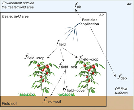
Illustration of initial pesticide distribution fractions to air (), off‐field surfaces (), field crop leaves (), cover crop leaves (), and field soil surface ()
After re‐arranging Equation (1), the fraction reaching the field surface area ( was obtained:
| (2) |
The fraction reaching the field surface area () is partially deposited on crop leaves () according to crop intercepted fraction and calculated as:
| (3) |
Then, the fraction left on the field after crop interception ( is calculated as:
| (4) |
The newly introduced fractions of pesticides reaching the cover leaves ( and the field soil are then calculated according to the effective area fraction of crop‐free field that is covered by cover crop ():
| (5) |
| (6) |
where is calculated by multiplying the area fraction of crop‐free field that is cover crop () and the area fraction of cover crop that is covered by leaves ():
| (7) |
Secondary emission fractions
Again building on the initial PestLCI mass balance (Dijkman et al., 2012) from the initial distribution fractions, secondary emissions processes occur. All processes defined in PestLCI for the main crop leaves were also applied to cover crop leaves, that is, degradation, uptake, and volatilization. The fractions degraded and volatilized were aggregated with the respective processes occurring on the main crop, ultimately affecting fractions emitted to air and field soil. A new emission output fraction, , was created to consider the uptake fraction by the cover leaves and the fraction remaining on cover leaves that was not yet taken up by the cover leaves.
The degradation on cover crop leaves was integrated in the total degraded fraction of pesticide. To consider the cover family (e.g., Pooideae), the degradation rate constant for pesticides on cover leaves () in (d−1) was calculated. Based on a database of measured dissipation half‐lives (Fantke & Juraske, 2013), the pesticide dissipation half‐life (d) on leaf cover at the average temperature in the month of application () was used as a proxy, and a dissipation half‐life model was derived, using a temperature coefficient (Fantke et al., 2014) to correct for actual field temperature. Thus, the following correction was applied to assess the dissipation half‐life on leaf cover at the average temperature in the month of application () as:
| (8) |
where is the pesticide half‐life on cover leaf at reference temperature (20 °C) (d), the average temperature in the month of application (°C), and the temperature at which the dissipation half‐life is reported (20 °C). is selected from a list of coefficients for crops that correspond to one of the relevant cover families (e.g., Pooideae).
Then, analogous to the pesticide translocation and removal processes implemented for the field crops, the degradation rate constant for pesticides on cover leaves at average temperature in the month of application (d−1) was calculated as:
| (9) |
Finally, the overall rate constant for the cover leaves (d−1) was calculated as:
| (10) |
where the rate constant for volatilization from the leaf surface, (d−1), and the rate constant for leaf uptake, (d−1), are both modeled independently of the crop or cover family, and where the degradation rate constant for pesticides on cover leaves, (d−1) is modeled according to Equation (9).
The processes of degradation, volatilization, and uptake on cover leaves are calculated until the time defined for the secondary emissions to occur after pesticide application (default: d).
Considering the crop family of the cover, the degradation on cover leaves ( is different from that on the main crop, and was calculated as:
| (11) |
where is the fraction reaching cover leaves after pesticide application, Equation (5); is the degradation rate constant for pesticides on leaf at average temperature in the month of application (d−1), Equation (9); and is the overall rate constant dissipation on cover leaves (d−1), Equation (10).
The volatilization on cover leaves ( was calculated as:
| (12) |
where is the fraction reaching cover leaves after pesticide application, Equation (5); is the rate constant for volatilization from the leaf surface (d−1); and is the overall rate constant dissipation on cover (d−1), Equation (10).
The cover leaves uptake ( was calculated as:
| (13) |
where is the fraction reaching cover leaves after pesticide application, Equation (5); is the rate constant for leaf uptake (d−1) independent of the crop or cover family; and is the overall rate constant dissipation on cover leaves, Equation (10).
The fraction remaining on cover leaves () that was not degraded, taken up, or volatilized at , was calculated as:
| (14) |
where is the fraction reaching cover leaves after pesticide application, Equation (5); and is the overall rate constant for removal from cover leaves (d−1), Equation (10).
The total fraction in and on cover leaves ( was calculated by summing the fraction uptake from cover leaves () and the fraction remaining on cover leaves ( as:
| (15) |
Other processes not affected by the presence of a cover crop (e.g., processes related to crop leaves) are detailed elsewhere (Dijkman et al., 2012).
Propagation of GCM to impact score level
To evaluate how the introduction of GCM influences final LCA results, impact scores (IS) for freshwater ecotoxicity impacts of pesticide emissions were calculated with USEtox (Rosenbaum et al., 2008), considering the application of 1 kg of pesticide on a tomato or grapevine field of 1 ha. The impact score ( in PAF m3 d/kgapplied) was calculated as:
| (16) |
where (kgemitted/kgapplied) is the total emitted mass of pesticide from the crop production into a given environmental compartment , and (PAF m3 d/kgemitted) is the corresponding characterization factor for freshwater ecotoxicity. Related impact characterization factors for freshwater ecotoxicity of the two considered pesticides (mancozeb and pyriproxyfen) are presented in Supporting Information, Table S2.
As recommended in Fantke et al. (2018) and applied in Gentil et al. (2020a), emissions to air were assigned in the impact assessment model USEtox to continental rural air; emissions to field soil were assigned to continental agricultural soil; and emissions to groundwater were assigned to continental freshwater. Off‐field surface emissions were assigned to continental agricultural soil, natural soil, and freshwater according to the typical area share of each compartment in a given region. Cover uptake fractions, along with crop uptake fractions and degradation, were not linked to the impact assessment when cover crop was considered to be removed from the field. Because the fractions of applied pesticides that are taken up into crops are subsequently harvested (field crops) or otherwise removed from the field (cover crops), these fractions are assumed not to reach the environment and hence do not contribute to impacts on ecosystems in our study. When cover crop was not removed from the field (e.g., buried), then impacts from pesticides present on the cover were attributed to the agricultural soil compartment. The fraction reaching the harvested field crop is attributed to a separate exposure pathway contributing to human toxicity impacts (Fantke et al., 2021).
Definition of illustrative case study under different conditions
To evaluate the proposed GC modeling approach, pesticide applications were simulated for grapevine (Vitis vinifera) in the Loire Valley in France (Figure 2A); following the initial work done on GCM in grapevine production in the Loire Valley by Renaud‐Gentié et al. (2015), and an open‐field tomato crop (Solanum lycopersicum) in the tropical conditions in Martinique in French West Indies (Figure 2B), for which a previous PestLCI model version was tested (Gentil et al., 2020a). With that, different conditions of crop, climate, soil, application method, and cover crop were considered (see Table 1). A default situation was defined for field characteristics and farming practices to allow feasible comparisons between crop production systems (i.e., field length and width of 100 m, no slope, no drift reduction system on the application method, no drainage system, no irrigation, and no tillage). Initial emissions to air () and to off‐field surfaces () were defined according to pesticide drift caused by the selected application method, that is, with a knapsack sprayer on tomato (García‐Santos et al., 2016) and with an air‐assisted sprayer side‐by‐side flat fan nozzles on grapevine (Codis et al., 2011). To estimate secondary emission fractions, a default time assessed at 1 day was considered.
Figure 2.
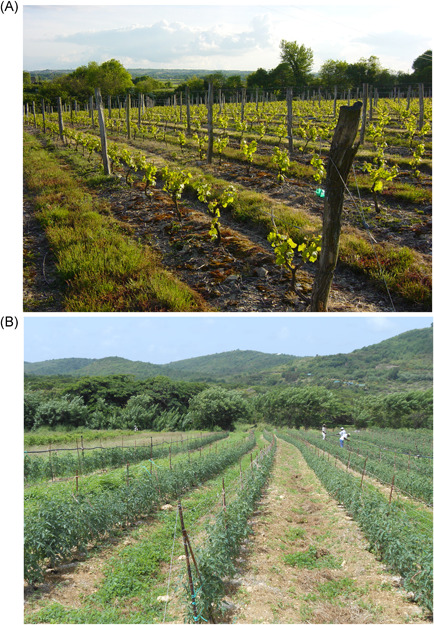
Cover crop planted on grapevine cultivation in Anjou, in the Loire Valley (A) and spontaneous cover on tomato production in Martinique, French West Indies (B)
Table 1.
Main characteristics of the case study and the two scenarios: grapevine and tomato production
| Crop | Grapevine | Tomato in open‐field | |
|---|---|---|---|
| Location | Loire Valley (France) | Martinique (French West Indies) | |
| Climate type and weather station | Marine West Coast Climate (Cfb)* ‐ Beaucouzé weather station | Tropical savanna climate (Aw)* ‐ Le Prêcheur, Météo France weather station | |
| Soil type | Sand on calcareous formation | Vitric andosol (FAO soil data) | |
| Application method | Air‐assisted sprayer side‐by‐side flat fan nozzles | Knapsack sprayer | |
| Cover crop family | Grass (Pooideae), Clover (Fabaceae) | Grass (Panicoideae), Stylosanthes guianensis (Fabaceae) | |
|
|
0.35 and 0.7 | ||
*From Köppen–Geiger climate classification.
To assess the variability of pesticide distribution on cover crop, different growth stages of the main crop () were considered, as well as the effective area fraction of crop‐free field that is cover cropped (). For each scenario, two main crop growth stages were considered, namely the leaf development and the flowering stage/development of fruit/ripening. They were defined as for leaf development and for flowering (Linders et al., 2000), corresponding to the crop growth stage of pesticide applications. Two types of cover crop were considered, a planted cover crop on the row of the main crop, , with a high pesticide interception fraction of (Renaud‐Gentié et al., 2015), and a spontaneous cover crop covering all field soil between the main crop with and a high pesticide interception fraction of . Therefore, the effective area fractions of cover crop are and . Each of the cover crops was composed of either grass from Pooideae or clover from the Fabaceae family for the grapevine production, and grass from Panicoideae or Stylosanthes guianensis from the Fabaceae family for the tomato production. Covers from Pooideae family are present mainly in temperate and dry climates, whereas covers from Panicoideae family dominate tropical and subtropical areas (Zuloaga et al., 2007). Cover crops of the Panicoideae and Pooideae families are grass, either planted or spontaneous, and cover crops from the Fabaceae family are legumes planted. The cover crop family is required to estimate the pesticide degradation on leaves (see Equation [8]). Generally, pesticide dissipates from leaves faster than from soil (Juraske et al., 2008) and varies according to plant family (Fantke & Juraske, 2013). Two pesticides homologated and used on tomato and grapevine were tested with contrasted dissipation half‐lives on soil and plant, with two target classes, namely the insecticide pyriproxyfen and the fungicide mancozeb. Because GCM is used partly to reduce the use of herbicides, which can also negatively affect the ground cover crops themselves, no herbicides were included in our case study. Their relevant physicochemical properties are detailed in Table S1.
Pesticide emissions were assigned in the impact assessment model USEtox. The off‐field deposition fraction was shared according to prevailing surface compartments in the region of each scenario using the CORINE Land Cover data (data.gouv.fr). In Martinique, the off‐field deposition fraction was allocated as follows: 29% to agricultural soil, 70% to natural soil, and 1% to freshwater, and in the Loire Valley, 67% to agricultural soil, 31.2% to natural soil, and 1.8% to freshwater.
Based on the calculation approach to emission distribution under GCM conditions, and the related calculation of ecotoxicity impacts in the case study, the effect of GCM on emission and related freshwater ecotoxicity impact results was analyzed.
Analysis of GCM effect on pesticide emissions and related impacts
To assess cover crop effects on initial and secondary distributions, control scenarios without cover (i.e., with bare soil) for each combination of pesticide, crop, and intercepted fractions (i.e., eight control scenarios with = 0) were designed and simulated. Distribution fractions are presented as a function of continuously increasing cover crop area fractions. After an analysis of the influence of the effective area fraction of cover crop on initial distribution fractions, a second analysis was carried out on the secondary emission fractions and particularly on processes involved on cover leaves, namely degradation, volatilization, and uptake.
At the impact level, scenarios with and without a cover crop were compared by calculating the percentage of change of for freshwater ecotoxicity (PAF m3 d/kgapplied), for each considered environmental emission compartment. The percentage of change () was calculated as:
| (17) |
When pesticide emissions to cover leaves are assigned to the agricultural soil compartment as field soil surface emissions, this corresponds for initial distribution fractions to a scenario without considering any cover. Therefore, the initial emission fraction reaching cover leaves, , was not linked to the impact assessment but considered as a removal process as for the pesticide emission on crop leaves. For secondary emissions, two agronomic situations were considered for the fraction taken up by the cover and left on cover leaves (. One situation considered that the cover crop was exported from the actual field crop, that is, mowed and transferred outside the field. Hence, was not linked to the impact assessment. The second situation considered the cover buried in the field soil by, for example, a tillage practice, so was assumed to reach agricultural soil as emission. In summary, three situations were analyzed: (i) initial distribution with cover exported from the field, (ii) secondary emissions with cover exported from the field, and (iii) secondary emissions with cover buried in the field soil.
RESULTS
Emission results
Across a range of effective area fractions of cover ( for the tomato and grapevine scenarios, the variability of initial and secondary distribution fractions is presented in Figure 3. Emission fractions for the two cover crops ( and ) are detailed in Table 2.
Figure 3.
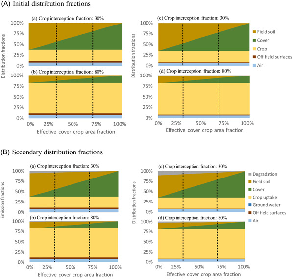
Initial (A) and secondary (B) emission distribution fractions for two crop growth stages, and , respectively, corresponding to the installation (a, c) and flowering stage (b, d), for grapevine (a, b) and tomato (c, d) for a range of effective area fractions of crop‐free field that is covered by cover crop (. Vertical lines represent the cover crop setup of the case study with and
Table 2.
Initial and secondary emission fractions for the tomato and grapevine production, for two crop growth stages, and , for the effective area fraction of crop‐free field that is covered by cover crop representing the two cover crop types with and (mean across scenarios)
| Crop → | Tomato | Grapevine | |||||||
|---|---|---|---|---|---|---|---|---|---|
| f intercept,crop → | 0.3 | 0.8 | 0.3 | 0.8 | |||||
|
↓ Distribution f eff,cover→ Compartment ↓ |
0.35 | 0.7 | 0.35 | 0.7 | 0.35 | 0.7 | 0.35 | 0.7 | |
| Initial | Air | 0.06 | 0.06 | 0.06 | 0.06 | 0.08 | 0.08 | 0.08 | 0.08 |
| Off‐field surfaces | 0.02 | 0.02 | 0.02 | 0.02 | 0.04 | 0.04 | 0.04 | 0.04 | |
| Crop leaves | 0.28 | 0.28 | 0.74 | 0.74 | 0.27 | 0.27 | 0.71 | 0.71 | |
| Field soil | 0.42 | 0.19 | 0.12 | 0.06 | 0.40 | 0.19 | 0.12 | 0.05 | |
| Cover leaves | 0.23 | 0.45 | 0.07 | 0.13 | 0.22 | 0.44 | 0.06 | 0.12 | |
| Secondary | Air | 0.06 | 0.06 | 0.06 | 0.06 | 0.08 | 0.08 | 0.08 | 0.08 |
| Off‐field surfaces | 0.02 | 0.02 | 0.02 | 0.02 | 0.04 | 0.04 | 0.04 | 0.04 | |
| Groundwater | 0 | 0 | 0 | 0 | 0 | 0 | 0 | 0 | |
| Field soil | 0.35 | 0.16 | 0.10 | 0.05 | 0.37 | 0.17 | 0.11 | 0.05 | |
| Degradation | 0.07 | 0.03 | 0.02 | 0.01 | 0.04 | 0.02 | 0.01 | 0.01 | |
| Crop uptake | 0.28 | 0.28 | 0.74 | 0.74 | 0.27 | 0.27 | 0.71 | 0.71 | |
| Cover | 0.23 | 0.45 | 0.07 | 0.13 | 0.22 | 0.43 | 0.06 | 0.12 | |
At initial distribution, the air‐assisted sprayer in grapevine displays higher off‐field surfaces emissions, and higher emission to air, , than the knapsack sprayer used in tomato production with and . The differences of emission fractions to air and off‐field surfaces are linked to the characteristics of the application method as discussed in Gentil‐Sergent et al. (2021). In the present case study, only agronomically relevant application methods were tested for each considered crop production system.
The initial pesticide distributions to soil and cover crop depend on the main crop intercepted fraction and the effective area fraction of cover. The higher the fraction intercepted by the crop (reproductive‐flowering phase), the lower the fraction distributed under the crop canopy (i.e., to the field soil and cover crop). Indeed, in our case study, when the main crop is starting to grow, the fraction of pesticide distributed between the soil and the cover crop was 3.5 times higher than when the main crop is at the flowering stage (Table 2). On average, the presence of a cover crop reduced the fraction reaching field soil by a factor of 3 compared with a bare soil regardless of the field crop, its growth stage, and the effective area fraction of cover. The variation in the fraction reaching field soil among scenarios was caused mainly by different effective area fractions of cover, driven by the area fraction of crop‐free field that is cover crop and the area fraction of cover crop that is covered by leaves corresponding to the cover leaves density. The higher the effective area fraction of cover, the lower the fraction distributed to field soil. The effect of cover crop on pesticide initial distribution fractions to field soil and cover crop was propagated to the secondary emission fractions (Figure 3).
When including secondary emission distribution processes, cover crop leaf uptake contributed more than 99% to cover‐crop‐related processes, yielding an average leaf uptake fraction of 0.22 across all scenarios. The total degraded fractions (on soil, on‐field crop, and cover leaves) in our case study were highest when there was no cover crop. This is explained by the fact that, despite faster degradation in crops and cover crops compared with soil, the even faster plant uptake into both crop and cover crop drives the overall pesticide distribution within 24 h that are considered in the emission model. Consequently, most of the pesticide is taken up into crop, while degradation processes will drive subsequent fate processes that are modeled as part of the impact assessment. The degraded fractions on cover leaves displayed only slight differences between the cover crop families, that is, Pooideae vs. Fabaceae for grapevine scenarios and Panicoideae vs. Fabaceae for tomato scenarios. Indeed, degradation on Fabaceae leaves was lower than on Pooideae and Panicoideae, owing to longer dissipation half‐lives on Fabaceae (see detail of DT50 in Table S3). On leaves, the only process considering crop and cover family is degradation. The fraction degraded on cover leaves was, on average, less than 0.1% but could reach a maximum of 0.65% for the mancozeb application with full coverage of Fabaceae (i.e., = 1). The fraction taken up by the cover that depends on the initial distribution fraction on cover leaves rose to approximately 18% when the crop growth stage was on maturation (), and rose to approximately 60% when the crop growth stage was on installation () for both scenarios.
The presence of a cover crop did not modify initial distribution fractions to air, crop, and off‐field surfaces. It did not modify either secondary emission fractions to off‐field surfaces, crop uptake, and fraction left on crop leaves. For secondary distribution scenarios, processes that are by default initiated after the first day after application were not included in our study but require further analysis to ensure consistency with our proposed GCM processes and to evaluate emissions eventually reaching groundwater or surface water. With that, the fractions emitted to off‐field surfaces did not vary with the presence or absence of a cover crop in our case study.
Overall, during initial and secondary distributions, the introduction of a cover crop with its own leaf surface area reduced the fraction reaching the field soil.
Impact results
The IS for the scenarios with a cover crop and the percentage of change compared with the scenarios without a cover (i.e., bare soil) are presented in Table 3. The contribution of the USEtox environmental compartments to the total IS calculated for the scenarios with and without cover crop for tomato and grapevine are presented in Figure 4 according to the distribution used (initial or secondary).
Table 3.
Impact score (IS, in units of PAF m3 d/kgapplied) of the average scenarios with a cover crop for each environmental compartment (continental: rural air, freshwater, natural soil, and agricultural soil), for the two scenarios: tomato and grapevine and %‐change (Equation 17) when not using a cover crop (i.e., bare soil), for the application of two pesticides (mancozeb and pyriproxyfen). Calculation of %‐change = [(IS_without_cover – IS_with_cover)/IS_with_cover] × 100
| Emission distribution and cover crop fate | Crop | IS Rural air | IS Freshwater | IS Natural soil | IS Agricultural Soil | Total |
|---|---|---|---|---|---|---|
| Initial distribution—with cover exported from the field* | Tomato | 21 (<1%) | 18 (−2%) | 10 (1%) | 201 (113%) | 251 (91%) |
| Grapevine | 26 (<1%) | 80 (−1%) | 11 (1%) | 214 (103%) | 331 (66%) | |
| Secondary emissions—cover exported from the field* | Tomato | 21 (<0.1%) | 18 (−) | 10 (−) | 189 (111%) | 238 (88%) |
| Grapevine | 26 (<0.1%) | 79 () | 11 (−) | 209 (100%) | 326 (64%) | |
| Secondary distribution—cover buried in the field soil** | Tomato | 21 (<0.1%) | 18 () | 10 (−) | 414 (−3%) | 463 (−3%) |
| Grapevine | 26 (<0.1%) | 79 () | 11 (−) | 424 (−2%) | 541 (−1%) |
and were not linked to the impact assessment model used (i.e., USEtox).
was assigned to continental agricultural soil in the impact assessment model used (i.e., USEtox).
Figure 4.

Contribution to total impact score expressed in PAF m3 d/kg pesticide applied, from each environmental compartment, for the tomato and grapevine scenarios, considering the presence of cover, using either the initial or secondary distribution, and indicating whether the fraction emitted to cover is assigned to agricultural soil or not (results are mean results obtained with the two pesticides)
Pesticide initial distribution fractions were assigned to the environmental compartments of the impact assessment model (i.e., USEtox), except the emission fractions to crop and cover leaves, because the plant compartment does not exist in the model. Only the impacts caused by agricultural soil emissions were affected by the consideration of a cover crop, with a reduction of approximately 100% regardless of crop type. As a consequence, the IS using initial distribution fractions were reduced by 65% for grapevine and by 90% for the tomato crop with the use of a cover crop.
Two connections were assessed between secondary emission fraction to cover and USEtox compartments. First, as for the connection with the initial distribution, no link to any USEtox compartment was assumed for the emission fraction to cover, considering cover exported from the field. Second, the fraction taken up by and present on cover leaves was assigned to agricultural soil, considering the cover buried in the field soil.
Using either initial or secondary distribution fractions, IS caused by emissions to the natural soil were not affected by cover crops; they are related to emissions from off‐field surfaces. In our two scenarios, the variation in IS to air with or without a cover was very small (. A variation of one order of magnitude was observed on the IS caused by emissions to air across scenarios caused by the vapor pressure of the two pesticides tested (see details of pesticide characteristics in Table S1). IS for emissions to continental freshwater (including emissions to ground and surface water) were not affected by the presence of a cover crop. In all scenarios, impact results based on secondary emission fractions were caused mainly by emissions to the continental agricultural soil compartment (Figure 4).
In all scenarios with and without cover crop, the total IS were higher on grapevine than on tomato. This is mainly the result of the higher emission fractions to off‐field surfaces for grapevine, with higher off‐field surfaces water area fraction in the Loire Valley (1.8%) than in Martinique (1%), and with higher characterization factors (CF) on emissions directly into the freshwater compartment than into other compartments (detail of CFs in Table S2).
Overall, across the two scenarios, the modeling of GCM demonstrated the potential to reduce emissions to field soil and related freshwater ecotoxicity impacts. This is because ecotoxicity impacts are driven mainly by pesticide fractions directly reaching surface water via deposition on off‐field areas as well as via fractions depositing on field soil and subsequently reaching water bodies. Moreover, when considering the cover exported from the field, and consequently not assigned to any environmental compartment in the impact assessment, total IS were reduced by approximately 65% (grapevine) and 90% (tomato) compared with bare soil scenarios for initial and secondary emissions. Conversely, when considering the cover buried in the field soil, total IS were similar to bare soil, reduced by only (grapevine) and (tomato).
DISCUSSION AND OUTLOOK
Applicability and limitations of the presented approach
The modeling of GCM in pesticide emission analysis was considered, by defining an effective area of cover and cover family, for initial and secondary pesticide distributions as derived with the PestLCI Consensus model. Within 1 day of assessment time after pesticide application, processes on cover leaves, that is, degradation, uptake, and volatilization, were modeled. The modeling of GCM fills a gap in the consideration of common farming practices, and demonstrated the potential of GCM to reduce emissions to field soil and related freshwater ecotoxicity impacts. Following our proposed approach to considering GCM processes, our emission results reproduce well the effect of GC on pesticide distribution as observed in cocoa farm systems by Vaikosen et al. (2019), where the reduction in bare soil surface with a GC of fallen leaves of the main crop decreased emission to the top soil. The higher the fraction of effective area of cover (composed of living or dead cover), the lower the fraction distributed to field soil.
Estimating pesticide interception by the crop or the cover crop is important to estimate pesticide losses to the environment (Lammoglia et al., 2016). Defining with the cover crop occupation fraction and the cover crop canopy fraction according to the growth stage of the cover allows estimating the pesticide interception by the cover crop, which could reach up to 60% during the installation phase of the main crop in our case study. Defining the crop intercepted fraction according to the LAI and the pesticide spraying technique for each crop family allows defining the intercepted fraction separately for the crop and the cover along the whole crop cycle and pesticide applications. As a consequence, the more precisely the fraction intercepted by the crop and the cover is defined, the better the estimate of the pesticide distribution for a living cover (Figure 3). The effective area fraction of cover should preferably be defined by observation. However, LCA practitioners rarely know the GCM and its characteristics. If the studied field cannot be visited, for crops grown in rows (e.g., orchards, grapevine) an effective area fraction of cover crop of can be assumed for a planted cover at its maximum development and an effective area fraction of for a spontaneous cover crop. Furthermore, a set of common living cover crops should be developed according to the main crop characteristics (e.g., on banana production at leaf development stage), defining the cover effective area fraction and the cover family.
After pesticide application, processes of degradation, uptake, and volatilization occur on the crop and cover leaves. To estimate the dissipation half‐lives on leaves, which are crop dependent (Fantke et al., 2014), the cover family (composed mostly of Pooideae, Panicoideae, or Fabaceae) has to be defined. For multispecies cover (e.g., weed development of multiple species), we recommend selecting the dominant cover crop family as reference.
In our two scenarios, the assignment of the emissions on the cover crop (uptake and left on leaves) to agricultural soil (considering the cover crop buried in the field) was compared with no assignment to any compartment (considering the cover exported from the field). The importance of the differences obtained with these two calculations (IS reduced by 65% for grapevine and by 90% for tomato when cover was not assigned to any environmental compartments as emission compared with assigned to field soil) needs to be relativized compared with the high uncertainty of the pesticide characterization factors for which uncertainties of 1–3 orders of magnitude apply (Rosenbaum et al., 2008). Notably, this is caused by the absence of modeling of the impact on soil life and pesticide metabolites (Notarnicola et al., 2017; van der Werf et al., 2020).
In the absence of complete sets of measured emission fractions to the environment, our proposed approach can only be qualitatively discussed, notably exploring other model design. Most pesticide transfer models at field scale (e.g., GLEAMS, MACRO, PEARL, PRZM) do not consider cover crop, and rather consider GC as plant residues (e.g., GLEAMS, PRZM; Mottes et al., 2014). Few models consider cover crops and associated pesticide transfer (i.e., R‐pest, WATPPASS) as proposed in this study. The R‐pest model coupled with SIMBA allows simulating banana and diverse cover crops and defining an indicator of pesticide risk exposure to surface and groundwater (Tixier et al., 2007; Tixier et al., 2011). The WATPPASS model, a hydrological model for small tropical volcanic catchments, allows the consideration of various types of ground cover, modifying environmental characteristics and thus pesticide transfers (Mottes, 2013; Mottes et al., 2015). As in those two models, the consideration of GCM in our proposed approach allows considering an important farming practice and its effects on pesticide transfer to the environment. Nevertheless, the outputs from those models cannot be compared with our emission fractions, mainly because they are not based on an emission mass balance as PestLCI Consensus.
To generalize our conclusions on GCM pesticide emissions and related impacts, a sensitivity analysis should be performed, notably testing the GCM modeling with a wide range of pesticides with diverse characteristics (e.g., DT50) and including additional environmental processes, climate conditions, and field crops as well as cover crop types. Furthermore, a wider range of crop types and related application methods should be tested in line with agronomically relevant practices. Overall, our proposal for modeling GCM raises awareness of the fraction of pesticides reaching living cover inside the field crop, which can affect the distribution of pesticides to the environment with its possible ecotoxicity impacts through agricultural soil emissions.
Future research needs
Additional research efforts are required on the modeling of processes occurring a few days after pesticide application (secondary distribution), with minimum redundancy with the impact assessment fate model. Modeling secondary distribution processes requires the accounting of local field, farming practices, soil and climate conditions, which are of particular interest to assess farming system diversity. Further research is required to consistently include additional processes, such as runoff, as well as to account for the influence of GCM on pesticide residues in edible field crops and on remaining pesticide fractions in unharvested cover crops.
More specifically, GC may affect water processes, such as runoff, leaching, or preferential flow (Alletto et al., 2010; Mottes et al., 2014; Reichenberger et al., 2007); thus, they can influence the affects. At emission level, GCM should reduce emissions to off‐field surfaces and to groundwater (Potter et al., 2007), and consequently, at impact level, total IS might be reduced for scenarios with a GC. Further research is therefore required to incorporate such processes consistently in our proposed GCM approach, as discussed in Gentil et al. (2020b), particularly for tropical crop production systems.
As recommended in Fantke et al. (2018), pesticide emissions were assigned to continental rural air, freshwater, agricultural soil, and natural soil compartments of the impact model USEtox. Recently, PestLCI initial distributions and the plant uptake and crop residue exposure model dynamiCROP (Fantke et al., 2011), which was recently adjusted for LCA (Fantke & Jolliet, 2016), were coupled (Gentil et al., 2020a), allowing the consideration of human toxicity caused by pesticides present in the harvested and consumed part of field crops. The pesticide deposited on non‐harvested living or dead plant, inside (e.g., cover crops) or outside the field (e.g., hedge tree), might have ecotoxicity impacts (Sharma et al., 2019) and require further research to be fully considered. Indeed, if crop residues and unharvested cover crop remain on the field, there could be further emissions to field soil and air, followed by subsequent transfer to freshwater compartments. The modeling of plant root uptake would be required to assess pesticide emissions to crop and cover crop residues (on the non‐harvested stem, roots, and leaves). If an LCA user assumes that the cover crop has been removed from the field, then impacts from pesticides present on the cover need to be assessed according to the subsequent processes applied to the cover.
As for the modeling of pesticide degradation on crop and cover leaves, volatilization and plant uptake should be refined to be modeled as a function of crop family, considering in particular leaf characteristics, which differ across crop types (Fantke & Juraske, 2013; Fantke et al., 2014).
Further improvement of GCM should be considered for modeling dead GC. Indeed, mulch or crop residues left on fields (e.g., stripping of banana while growing) are used largely in tropical conditions to keep moisture or reduce soil erosion (Lewis et al., 2016). At the initial distribution stage, all types of GC (living or dead mulch) can be modeled, by defining the effective area fraction of cover ( At the secondary distribution stage, specificities of the dead cover must be considered and modeled. Mulch is generally modeled as the first soil layer (Mottes et al., 2015) with its own characteristics notably of composition and degradation rate (Cassigneul et al., 2015). Plastic mulches are also used on vegetable production, or on pineapple production for example, generating specific water flows and consequently requiring specific modeling (Dusek et al., 2010). The inclusion of dead covers would be an important future step forward for modeling different types of GCM in the estimation of pesticide emissions in LCA and elsewhere.
Overall, the modeling of GC opened the path to the modeling of pesticide emissions in intercropping systems. This is particularly important because these systems are widely conducted in market gardening in tropical conditions to ensure income stability (Malézieux et al., 2009), increase crop yield per hectare, and optimize field conditions for growing certain crops (e.g., banana and cocoa).
CONCLUSIONS
The inclusion of GCM in pesticide emission modeling was proposed, defining an effective area of cover and the cover family through initial and secondary pesticide distributions. Across the two scenarios on tomato production in Martinique and on grapevine cultivation in the Loire Valley, the modeling of GCM allowed highlighting the potential of soil cover to reduce pesticide emissions and related freshwater ecotoxicity impacts. Including a new fraction on and in cover crop leaves, the emissions to field soil decreased by a factor of 3. During the secondary distribution, over the three processes occurring on the cover leaves, the fraction taken up by the cover leaves was predominant with more than 99% contribution to these processes. At both initial and secondary distribution levels, considering the cover exported from the field and consequently not assigned to any environmental emission compartment, total IS were reduced by approximately 65% and 90% compared with bare soil, for grapevine and tomato, respectively. Additional processes, such as runoff, should be considered in future efforts, along with accounting for the influence of GCM on pesticide residues in edible field crops and on remaining pesticide fractions in unharvested cover crops. Indeed, if crop residues and unharvested cover crop remain on the field, there could be further emissions to soil and air. The inclusion of dead cover would be an important step toward achieving the modeling of various types of GCM.
From the initial work of Renaud‐Gentié et al. (2015) on vines, the consideration of GCM as common farming practice opened the possibility of modeling it more widely for all crops with living cover crop. The modeling of living cover crop also opened the path toward the modeling of pesticide emissions in intercropping systems, widely conducted in market gardening, particularly in tropical regions. With that, our proposed approach constitutes a valuable starting point for addressing GCM practices in emission and impact assessments applied in LCA and elsewhere.
CONFLICT OF INTEREST
The authors declare no conflicts of interest.
SUPPORTING INFORMATION
The supporting information file contains information and characteristics of the pesticides used in the case study.
Supporting information
This article contains online‐only Supporting Information.
The supplemental data file contains information and characteristics of the pesticides used in the case study.
ACKNOWLEDGMENT
This work was financially supported by ADEME Martinique through the InnovACV project (No. 17MAC0038), CIRAD via the Rivage project funded by Martinique's European Regional Development Fund (MQ0003772‐CIRAD), ADEME France via the OLCA‐Pest project (grant agreement No. 17‐03‐C0025), the SPRINT Project (Grant Agreement 862568) funded by the European Commission through Horizon 2020, and the FNS‐Cloud Project (Grant Agreement 863059) funded by the European Commission through Horizon 2020.We thank Thomas Nemecek, Philippe Roux, Assumpció Antón, Nancy Peña, and Pierre Naviaux from the OLCA‐Pest project team for their feedback on an earlier version of the manuscript.
DATA AVAILABILITY STATEMENT
The model is available at https://pestlciweb.man.dtu.dk/. Further information is available upon request from corresponding author Peter Fanke (pefan@dtu.dk).
REFERENCES
- Abad, J. , Mendoza, I. H. , , de Marín, D. , Orcaray, L. , & Santesteban, L. G. (2021). Cover crops in viticulture. A systematic review (1): Implications on soil characteristics and biodiversity in vineyard. OENO One, 55(1), 295–312. 10.20870/oeno-one.2021.55.1.3599 [DOI] [Google Scholar]
- Alletto, L. , Coquet, Y. , Benoit, P. , Heddadj, D. , & Barriuso, E. (2010). Tillage management effects on pesticide fate in soils. A review. Agronomy for Sustainable Development, 30(2), 367–400. 10.1051/agro/2009018 [DOI] [Google Scholar]
- Ambiaud, E. (2012). Moins de désherbants dans les vignes. Agreste Primeur, (288),8 pages.
- Andersson, K. (2000). LCA of food products and production systems. International Journal of Life Cycle, 5(4), 239–248. 10.1007/BF02979367 [DOI] [Google Scholar]
- Bessou, C. , Basset‐Mens, C. , Tran, T. , & Benoist, A. (2013). LCA applied to perennial cropping systems: A review focused on the farm stage. International Journal of Life Cycle Assessment, 18(2), 340–361. 10.1007/s11367-012-0502-z [DOI] [Google Scholar]
- Birkved, M. , & Hauschild, M. Z. (2006). PestLCI—A model for estimating field emissions of pesticides in agricultural LCA. Ecological Modelling, 198(3), 433–451. 10.1016/j.ecolmodel.2006.05.035 [DOI] [Google Scholar]
- Cassigneul, A. , Alletto, L. , Benoit, P. , Bergheaud, V. , Etiévant, V. , Dumény, V. , Le Gac, A. L. , Chuette, D. , Rumpel, C. , & Justes, E. (2015). Nature and decomposition degree of cover crops influence pesticide sorption: Quantification and modelling. Chemosphere, 119, 1007–1014. 10.1016/j.chemosphere.2014.08.082 [DOI] [PubMed] [Google Scholar]
- CIRAD. (2009). Mémento de l'agronome. Ed. Quae. http://agritrop.cirad.fr/558543/
- Codis, S. , Bos, C. , & Laurent, S. (2011). Réduction de la dérive, 8 matériels testés sur vigne. Phytoma, 640, 1–5. [Google Scholar]
- DAAF Martinique . (2018). Pratiques culturales en 2015: Kou d'zyé sur celles de la banane en Martinique. Dossiers Agreste Martinique. (n° 11).
- Dijkman, T. J. , Birkved, M. , & Hauschild, M. Z. (2012). PestLCI 2.0: A second generation model for estimating emissions of pesticides from arable land in LCA. International Journal of Life Cycle Assessment, 17(8), 973–986. 10.1007/s11367-012-0439-2 [DOI] [Google Scholar]
- Durán Zuazo, V. H. , & Rodríguez Pleguezuelo, C. R. (2008). Soil‐erosion and runoff prevention by plant covers. A review. Agronomy for Sustainable Development, 28(1), 65–86. 10.1051/agro:2007062 [DOI] [Google Scholar]
- Dusek, J. , Ray, C. , Alavi, G. , Vogel, T. , & Sanda, M. (2010). Effect of plastic mulch on water flow and herbicide transport in soil cultivated with pineapple crop: A modeling study. Agricultural Water Management, 97(10), 1637–1645. 10.1016/j.agwat.2010.05.019 [DOI] [Google Scholar]
- Fantke, P. , Antón, A. , Grant, T. , & Hayashi, K. (2017). Pesticide emission quantification for life cycle assessment: A global consensus building process. The International Journal of Life Cycle Assessment, 13(3), 245–251. [Google Scholar]
- Fantke, P. , Aurisano, N. , Bare, J. , Backhaus, T. , Bulle, C. , Chapman, P. M. , De Zwart, D. , Dwyer, R. , Ernstoff, A. , Golsteijn, L. , Holmquist H., Jolliet O., McKone T.E., Owsianiak M., Peijnenburg W., Posthuma L., Roos S., Saouter E., Schowanek D., … Hauschild M. (2018). Toward harmonizing ecotoxicity characterization in life cycle impact assessment. Environmental Toxicology and Chemistry, 37(12), 2955–2971. 10.1002/etc.4261 [DOI] [PMC free article] [PubMed] [Google Scholar]
- Fantke, P. , Chiu, W. A. , Aylward, L. , Judson, R. , Huang, L. , Jang, S. , Gouin, T. , Rhomberg, L. , Aurisano, N. , McKone, T. , & Jolliet O. (2021). Exposure and toxicity characterization of chemical emissions and chemicals in products: global recommendations and implementation in USEtox. International Journal of Life Cycle Assessment, 26, 899– 915. 10.1007/s11367-021-01889-y [DOI] [PMC free article] [PubMed] [Google Scholar]
- Fantke, P. , Gillespie, B. W. , Juraske, R. , & Jolliet, O. (2014). Estimating half‐lives for pesticide dissipation from plants. Environmental Science and Technology, 48(15), 8588–8602. 10.1021/es500434p [DOI] [PubMed] [Google Scholar]
- Fantke, P. , & Jolliet, O. (2016). Life cycle human health impacts of 875 pesticides. International Journal of Life Cycle Assessment, 21(5), 722–733. 10.1007/s11367-015-0910-y [DOI] [Google Scholar]
- Fantke, P. , & Juraske, R. (2013). Variability of pesticide dissipation half‐lives in plants. Environmental Science and Technology, 47(8), 3548–3562. 10.1021/es303525x [DOI] [PubMed] [Google Scholar]
- Fantke, P. , Juraske, R. , Antón, A. , Friedrich, R. , & Jolliet, O. (2011). Dynamic multicrop model to characterize impacts of pesticides in food. Environmental Science and Technology, 45(20), 8842–8849. 10.1021/es201989d [DOI] [PubMed] [Google Scholar]
- García‐Santos, G. , Feola, G. , Nuyttens, D. , & Diaz, J. (2016). Drift from the use of hand‐held knapsack pesticide sprayers in Boyacá (Colombian Andes). Journal of Agricultural and Food Chemistry, 64(20), 3990–3998. 10.1021/acs.jafc.5b03772 [DOI] [PubMed] [Google Scholar]
- Gentil, C. , Basset‐Mens, C. , Manteaux, S. , Mottes, C. , Maillard, E. , Biard, Y. , & Fantke, P. (2020a). Coupling pesticide emission and toxicity characterization models for LCA: Application to open‐field tomato production in Martinique. Journal of Cleaner Production, 277, 124099. 10.1016/j.jclepro.2020.124099 [DOI] [Google Scholar]
- Gentil, C. , Fantke, P. , Mottes, C. , & Basset‐Mens, C. (2020b). Challenges and ways forward in pesticide emission and toxicity characterization modeling for tropical conditions. International Journal of Life Cycle Assessment, 25(7), 1290–1306. 10.1007/s11367-019-01685-9 [DOI] [Google Scholar]
- Gentil‐Sergent, C. , Basset‐Mens, C. , Gaab, J. , Mottes, C. , Melero, C. , & Fantke, P. (2021). Quantifying pesticide emission fractions for tropical conditions. Chemosphere, 275, 130014. 10.1016/j.chemosphere.2021.130014 [DOI] [PubMed] [Google Scholar]
- Griggs, D. , Stafford‐Smith, M. , Gaffney, O. , Rockström, J. , Öhman, M. C. , Shyamsundar, P. , Steffen, W. , Glaser, G. , Kanie, N. , & Noble, I. (2013). Sustainable development goals for people and planet. Nature, 495(7441), 305–307. 10.1038/495305a [DOI] [PubMed] [Google Scholar]
- HLPE . (2019). Agroecological and other innovative approaches for sustainable agriculture and food systems that enhance food security and nutrition. A report by the High Level Panel of Experts on Food Security and Nutrition of the Committee on World Food Security:163.
- Juraske, R. , Antón, A. , & Castells, F. (2008). Estimating half‐lives of pesticides in/on vegetation for use in multimedia fate and exposure models. Chemosphere, 70(10), 1748–1755. 10.1016/j.chemosphere.2007.08.047 [DOI] [PubMed] [Google Scholar]
- Lammoglia, S.‐K. , Moeys, J. , Barriuso, E. , Larsbo, M. , Marín‐Benito, J.‐M. , Justes, E. , Alletto, L. , Ubertosi, M. , Nicolardot, B. , Munier‐Jolain, N. , & Mamy L. (2016). Sequential use of the STICS crop model and of the MACRO pesticide fate model to simulate pesticides leaching in cropping systems. Environmental Science and Pollution Research, 24(8), 6895–6909. 10.1007/s11356-016-6842-7 [DOI] [PubMed] [Google Scholar]
- Lewis, S. E. , Silburn, D. M. , Kookana, R. S. , & Shaw, M. (2016). Pesticide behavior, fate, and effects in the tropics: An overview of the current state of knowledge. Journal of Agricultural and Food Chemistry, 64(20), 3917–3924. 10.1021/acs.jafc.6b01320 [DOI] [PubMed] [Google Scholar]
- Linders, J. , Mensink, H. , Stephenson, G. , Wauchope, D. , & Racke, K. (2000). Foliar interception and retention values after pesticide application: A proposal for standardised values for environmental risk assessment. Pest Management Science, 58(3), 315–315. 10.1002/ps.448 [DOI] [Google Scholar]
- Meier, M. S. , Stoessel, F. , Jungbluth, N. , Juraske, R. , Schader, C. , & Stolze, M. (2015). Environmental impacts of organic and conventional agricultural products—Are the differences captured by life cycle assessment. Journal of Environmental Management, 149, 193–208. 10.1016/j.jenvman.2014.10.006 [DOI] [PubMed] [Google Scholar]
- Meier, U. (2018). Growth stages of mono‐ and dicotyledonous plants: BBCH Monograph. Open Agrar Repositorium. https://www.openagrar.de/receive/openagrar_mods_00042351
- Mottes, C. (2013). Evaluation des effets des systèmes de culture sur l'exposition aux pesticides des eaux à l'exutoire d'un bassin versant. Proposition d'une méthodologie d'analyse appliquée au cas de l'horticulture en Martinique. [Paris]: AgroParisTech.
- Mottes, C. , Lesueur Jannoyer, M. , Le Bail, M. , Guéné, M. , Carles, C. , & Malézieux, E. (2017). Relationships between past and present pesticide applications and pollution at a watershed outlet: The case of a horticultural catchment in Martinique, French West Indies. Chemosphere, 184, 762–773. 10.1016/j.chemosphere.2017.06.061 [DOI] [PubMed] [Google Scholar]
- Mottes, C. , Lesueur‐Jannoyer, M. , Bail, M. L. , & Malézieux, E. (2014). Pesticide transfer models in crop and watershed systems: A review. Agronomy for Sustainable Development, 34(1), 229–250. 10.1007/s13593-013-0176-3 [DOI] [Google Scholar]
- Mottes, C. , Lesueur‐Jannoyer, M. , Charlier, J.‐B. , Carles, C. , Guéné, M. , Le Bail, M. , & Malézieux, E. (2015). Hydrological and pesticide transfer modeling in a tropical volcanic watershed with the WATPPASS model. Journal of Hydrology, 529(Part 3), 909–927. 10.1016/j.jhydrol.2015.09.007 [DOI] [Google Scholar]
- Nemecek, T. , & Schnetzer, J. (2011). Methods of assessment of direct field emissions for LCIs of agricultural production systems. Data v3.0. Duebendord, Switzerland: Swiss Center for Life Cycle Inventories.
- Neto, B. , Dias, A. C. , & Machado, M. (2013). Life cycle assessment of the supply chain of a Portuguese wine: From viticulture to distribution. International Journal of Life Cycle Assessment, 18(3), 590–602. 10.1007/s11367-012-0518-4 [DOI] [Google Scholar]
- Notarnicola, B. , Sala, S. , Antón, A. , McLaren, S. J. , Saouter, E. , & Sonesson, U. (2017). The role of life cycle assessment in supporting sustainable agri‐food systems: A review of the challenges. Journal of Cleaner Production, 140(Part 2), 399–409. 10.1016/j.jclepro.2016.06.071 [DOI] [Google Scholar]
- Oliquino‐Abasolo, A. (2015). Agro‐environmental sustainability of conventional and organic vegetable production systems in Tayabas, Quezon, Philippines. FAO. University Library, University of the Philippines at Los Baños. http://agris.fao.org/agris-search/search.do?recordID=PH2018000866
- Perrin, A. , Basset‐Mens, C. , & Gabrielle, B. (2014). Life cycle assessment of vegetable products: A review focusing on cropping systems diversity and the estimation of field emissions. International Journal of Life Cycle Assessment, 19(6), 1247–1263. 10.1007/s11367-014-0724-3 [DOI] [Google Scholar]
- Poore, J. , & Nemecek, T. (2018). Reducing food's environmental impacts through producers and consumers. Science, 360(6392), 987–992. 10.1126/science.aaq0216 [DOI] [PubMed] [Google Scholar]
- Potter, T. L. , Bosch, D. D. , Joo, H. , Schaffer, B. , & Muñoz‐Carpena, R. (2007). Summer cover crops reduce atrazine leaching to shallow groundwater in Southern Florida. Journal of Environmental Quality, 36(5), 1301–1309. 10.2134/jeq.2006.0526 [DOI] [PubMed] [Google Scholar]
- Reichenberger, S. , Bach, M. , Skitschak, A. , & Frede, H.‐G. (2007). Mitigation strategies to reduce pesticide inputs into ground‐ and surface water and their effectiveness: A review. Science of the Total Environment, 384(1–3), 1–35. 10.1016/j.scitotenv.2007.04.046 [DOI] [PubMed] [Google Scholar]
- Renaud‐Gentié, C. , Dieu, V. , Thiollet‐Scholtus, M. , & Mérot, A. (2020). Addressing organic viticulture environmental burdens by better understanding interannual impact variations. International Journal of Life Cycle Assessment, 25(7), 1307–1322. 10.1007/s11367-019-01694-8 [DOI] [Google Scholar]
- Renaud‐Gentié, C. , Dijkman, T. J. , Bjørn, A. , & Birkved, M. (2015). Pesticide emission modelling and freshwater ecotoxicity assessment for Grapevine LCA: Adaptation of PestLCI 2.0 to viticulture. International Journal of Life Cycle Assessment, 20(11), 1528–1543. 10.1007/s11367-015-0949-9 [DOI] [Google Scholar]
- Rosenbaum, R. K. , Bachmann, T. M. , Gold, L. S. , Huijbregts, M. A. J. , Jolliet, O. , Juraske, R. , Koehler, A. , Larsen, H. F. , MacLeod, M. , Margni, M. , McKone, T. E. , Payet, J. , Schuhmacher, M. , van de Meent, D. , & Hauschild, M. Z. (2008). USEtox—The UNEP‐SETAC toxicity model: Recommended characterisation factors for human toxicity and freshwater ecotoxicity in life cycle impact assessment. International Journal of Life Cycle Assessment, 13(7), 532–546. 10.1007/s11367-008-0038-4 [DOI] [Google Scholar]
- Rouault, A. , Beauchet, S. , Renaud‐Gentie, C. , & Jourjon, F. (2016). Life cycle assessment of viticultural technical management routes (TMRs): comparison between an organic and an integrated management route. OENO One, 50(2). 10.20870/oeno-one.2016.50.2.783 https://oeno-one.eu/article/view/783 [DOI] [Google Scholar]
- Rouault, A. , Perrin, A. , Renaud‐Gentié, C. , Julien, S. , & Jourjon, F. (2020). Using LCA in a participatory eco‐design approach in agriculture: The example of vineyard management. International Journal of Life Cycle Assessment, 25(7), 1368–1383. 10.1007/s11367-019-01684-w [DOI] [Google Scholar]
- Roy, P. , Nei, D. , Orikasa, T. , Xu, Q. , Okadome, H. , Nakamura, N. , & Shiina, T. (2009). A review of life cycle assessment (LCA) on some food products. Journal of Food Engineering, 90(1), 1–10. 10.1016/j.jfoodeng.2008.06.016 [DOI] [Google Scholar]
- Sharma, A. , Kumar, V. , Thukral, A. K. , & Bhardwaj, R. (2019). Responses of plants to pesticide toxicity: An Overview. Planta Daninha, 37, 37. 10.1590/s0100-83582019370100065 [DOI] [Google Scholar]
- Shaxson, F. (1999). New concepts and approaches to land management in the tropics with emphasis on steeplands. FAO. [Google Scholar]
- Tixier, P. , Lavigne, C. , Alvarez, S. , Gauquier, A. , Blanchard, M. , Ripoche, A. , & Achard, R. (2011). Model evaluation of cover crops, application to eleven species for banana cropping systems. European Journal of Agronomy, 34(2), 53–61. 10.1016/j.eja.2010.10.004 [DOI] [Google Scholar]
- Tixier, P. , Malézieux, E. , Dorel, M. , Bockstaller, C. , & Girardin, P. (2007). Rpest—An indicator linked to a crop model to assess the dynamics of the risk of pesticide water pollution. European Journal of Agronomy, 26(2), 71–81. 10.1016/j.eja.2006.08.006 [DOI] [Google Scholar]
- Tscharntke, T. , Clough, Y. , Wanger, T. C. , Jackson, L. , Motzke, I. , Perfecto, I. , Vandermeer, J. , & Whitbread, A. (2012). Global food security, biodiversity conservation and the future of agricultural intensification. Biological Conservation, 151(1), 53–59. 10.1016/j.biocon.2012.01.068 [DOI] [Google Scholar]
- Vaikosen, E. N. , Olu‐Owolabi, B. I. , Gibson, L. T. , Adebowale, K. O. , Davidson, C. M. , & Asogwa, U. (2019). Kinetic field dissipation and fate of endosulfan after application on Theobroma cacao farm in tropical Southwestern Nigeria. Environmental Monitoring and Assessment, 191(3), 191–196. 10.1007/s10661-019-7293-7 [DOI] [PubMed] [Google Scholar]
- Watson, D. J. (1947). Comparative physiological studies on the growth of field crops. I. Variation in net assimilation rate and leaf area between species and varieties, and within and between years. Annals of Botany, 11, 41–76. [Google Scholar]
- van der Werf, H. M. G. , Knudsen, M. T. , & Cederberg, C. (2020). Towards better representation of organic agriculture in life cycle assessment. Nature Sustainability, 3(6), 419–425. 10.1038/s41893-020-0489-6 [DOI] [Google Scholar]
- Wezel, A. , Casagrande, M. , Celette, F. , Vian, J.‐F. , Ferrer, A. , & Peigné, J. (2014). Agroecological practices for sustainable agriculture. A review. Agronomy for Sustainable Development, 34(1), 1–20. 10.1007/s13593-013-0180-7 [DOI] [Google Scholar]
- Zuloaga, F. , Morrone, O. , Davidse, G. , & Pennington, S. (2007). Classification and Biogeography of panicoideae (Poaceae) in the new world. Aliso: A Journal of Systematic and Evolutionary Botany, 23(1), 503–529. 10.5642/aliso.20072301.39 [DOI] [Google Scholar]
Associated Data
This section collects any data citations, data availability statements, or supplementary materials included in this article.
Supplementary Materials
This article contains online‐only Supporting Information.
The supplemental data file contains information and characteristics of the pesticides used in the case study.
Data Availability Statement
The model is available at https://pestlciweb.man.dtu.dk/. Further information is available upon request from corresponding author Peter Fanke (pefan@dtu.dk).