Estimation of the generation interval using pairwise relative transmission probabilities

Summary

The generation interval (the time between infection of primary and secondary cases) and its often used proxy, the serial interval (the time between symptom onset of primary and secondary cases) are critical parameters in understanding infectious disease dynamics. Because it is difficult to determine who infected whom, these important outbreak characteristics are not well understood for many diseases. We present a novel method for estimating transmission intervals using surveillance or outbreak investigation data that, unlike existing methods, does not require a contact tracing data or pathogen whole genome sequence data on all cases. We start with an expectation maximization algorithm and incorporate relative transmission probabilities with noise reduction. We use simulations to show that our method can accurately estimate the generation interval distribution for diseases with different reproductive numbers, generation intervals, and mutation rates. We then apply our method to routinely collected surveillance data from Massachusetts (2010–2016) to estimate the serial interval of tuberculosis in this setting.

1. Introduction

The generation interval, defined as the time from infection of the source case (i.e., the infector) to infection of their secondary case (i.e., the infectee), is an important infectious disease characteristic. This parameter is used to estimate another important characteristic, the reproductive number, defined as the average number of secondary cases produced by a primary case over the course of their infection (Cauchemez and others, 2006; Wallinga and Teunis, 2004; Champredon and Dushoff, 2015; Park and others, 2019). The generation interval is also used to model possible transmission trees for an infectious disease outbreak (Hall and others, 2015; Jombart and others, 2014; Campbell and others, 2019).

In practice, the exact infection time is rarely known so the serial interval, i.e., the time between onset of symptoms in the source and secondary cases, is often used as a proxy for the generation interval, though how good a proxy the serial interval is depends on many factors (Svensson, 2007; Pavlin, 2014; Britton and Tomba, 2019). Estimating these transmission intervals is difficult for numerous reasons including identifying transmission pairs, censoring, and unknown infection/symptom onset times. Therefore, estimates of these quantities are rare and/or inconsistent for many diseases (Ma and others, 2018; Vink and others, 2014). Most methods to estimate transmission intervals use household contact studies or detailed contact investigations where one can more easily identify transmission pairs (Borgdorff and others, 2011; Brooks-Pollock and others, 2011; Cowling and others, 2009; Ma and others, 2020). However, household contact studies are often limited in size and do not account for community transmission, making methods to estimate the generation interval using surveillance data an important research area.

White and Pagano (2008) developed a method to estimate the reproductive number and transmission interval simultaneously using surveillance data, which has been extended by others (Becker and others, 2010; Moser and others, 2015). However, Griffin and others (2011) showed that the joint estimation of both parameters can be difficult in certain settings. Other studies, such as Didelot and others (2017) and Klinkenberg and others (2017), use pathogen whole-genome sequence (WGS) data to estimate the generation interval distribution. However, those methods can only be applied to datasets with nearly complete WGS data. Hens and others (2012) developed a flexible method to estimate the serial interval using pairwise transmission probabilities. However, their method requires limits on the number of possible infectors to prevent the noise of the unlinked pairs from overwhelming the signal of the truly linked pairs.

We aimed to develop a way to estimate transmission intervals from surveillance data where there is limited WGS and/or contact investigation data. Our work was motivated by a rich tuberculosis (TB) surveillance dataset from Massachusetts state, which includes all TB cases reported 2010–2016. We used a method developed by Hens and others (2012) and extended it to incorporate relative transmission probabilities estimated by a novel method which integrates multiple data sources (Leavitt and others, 2020). We then estimated the serial interval and reproductive number for TB in Massachusetts.

2. Statistical methods

Our methods can be used to estimate any transmission interval depending on the dates used: the generation interval with infection dates, the serial interval with symptom onset dates, or more generic transmission intervals if only observation dates are known. We will describe the methods in this last, most generic case.

2.1. Generation interval estimation

We consider an outbreak investigation or surveillance dataset that contains cases, , ordered by observation date so that case was the first case observed. The transmission interval for case is the time between observation of case , and observation of its infector, . We call this transmission interval 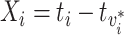, where is the observation time of case . We assume that are independent and identically distributed according to a density . This and subsequent notation is detailed in Table 1. 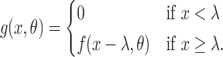Any density can be used, but here, we assume is a gamma distribution with , where is the shape parameter and is the scale parameter. We also allow for a transmission interval distribution that has a pre-specified shift, , to exclude coprevalent cases (cases identified close in time so that it cannot be determined who was observed first) forcing the transmission interval distribution to be greater than

(2.1)

Table 1.

Notation for transmission interval estimation method

Symbol	Meaning
	Total number of cases
	Vector of possible infectors of case with length
	True infector of case
	Observation time of case
	Distribution of the transmission intervals
	Shape parameter for a gamma transmission interval distribution
	Scale parameter for a gamma transmission interval distribution
	Shift of the gamma transmission interval distribution
	True transmission interval for case
	Vector of all transmission intervals
	Vector of all observed transmission intervals
	Vector of all unobserved transmission intervals
	Number of unobserved transmission intervals
	Matrix of covariates for case and all possible infectors informing
	the probability of the cases interacting
	Prior probability that case was infected by case
	Cluster of high probability infectors
	Cluster of remaining infectors
	The empirical cumulative density function for the probabilities
	of the infectors of case
	The kernel density estimate for the probabilities
	of the infectors of case
	The binwidth parameter for kernel density estimation
	The mean, median, or sd of the transmission interval distribution
	The quantile function of the bootstrap estimates of

If we knew all true transmission pairs, then estimation of the transmission interval would be a simple maximum likelihood estimation problem. The observed transmission intervals, , would be used to maximize the likelihood

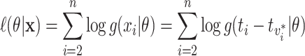(2.2)

to find . Note that the indexing starts at case , because since case is the first case in our sample, the infector is unknown. However, in practice, we do not know the true infectors and therefore, a more sophisticated approach is needed.

2.2. PEM algorithm: Hens and others (2012)

Hens and others (2012) developed a way to estimate transmission intervals using the expectation maximization (EM) algorithm to account for the fact that the transmission intervals for most cases are unobserved. They split the random vector of all transmission intervals, , into a vector of observed, , and unobserved, , transmission intervals where there are unobserved transmission intervals. The authors define observed transmission intervals as the transmission intervals for cases with only one possible infector. The complete log likelihood then becomes

(2.3)

The Q function for the E-Step is then derived by taking the expected likelihood over

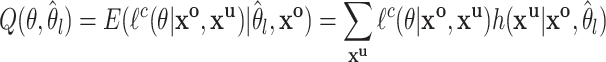(2.4)

where is the current estimate of the interval parameters and is the distribution of the unobserved transmission intervals. The M-step is then given by .

Summing over is the same as summing over all observed transmission intervals with each possible infector the case. Therefore, assuming that the observed and unobserved transmission intervals are independent given , we set , where equals the relative probability that case was infected by case . The authors called their method the prior-based expectation maximization (PEM) algorithm because they used prior information about the probability that the cases and interacted, , to calculate with

(2.5)

where is a vector of all possible infectors of case and represents the information about interaction between case and all possible infectors. The Q function can then be re-written as

(2.6)

This simplification is detailed in the supplementary material available at Biostatistics online.

2.3. Incorporating naive Bayes transmission probabilities

In their paper, Hens and others (2012) used details from contact investigations to inform their prior estimates of . We take a different approach and use the relative transmission probabilities estimated by a machine learning method, naive Bayes, from a combination of genetic, spatial, clinical, and demographic data, described in detail in Leavitt and others (2020). Briefly, a training set of probable links and nonlinks defined by either pathogen WGS and/or contact investigation data from a subset of the cases is used to estimate the probability that pairs have different covariates given if they are linked or not. Then Bayes rule is used to predict the probability all ordered pairs of cases are linked given their covariates. The method uses an iterative procedure account for the uncertainty in the training set; including the training pairs in the prediction set so that the transmission probability for these pairs is estimated as well.

The probabilities estimated from naive Bayes have the correct form to be used in the Hens and others (2012) method. However, in their paper the authors limited the possible infectors, , to only confirmed contacts of case , resulting in very few possible infectors per case. On the other hand, the naive Bayes transmission method only limits to cases infected before case . Consider the ideal scenario of a completely sampled outbreak, we would observe 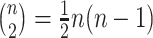generation intervals of which only of them would be from true transmission pairs. Even if the method assigns low probabilities to all of the incorrect infectors, these probabilities will nonetheless be non-zero and the sheer magnitude of them will still overwhelm the signal of the true pairs. Therefore, by not limiting to only a few possible infectors through using confirmed contacts as Hens and others (2012) did, we need to reduce to maximize the signal to noise ratio.

2.4. Clustering possible infectors

To reduce the noise, we use clustering to identify cases for which there is a group of high probability infectors that is distinct from the rest of the infectors. Then, we limit to only that high probability cluster of infectors as shown in case A in Figure 1. If a case has no clear high probability cluster like case B in Figure 1, we exclude that case because we have low confidence in which observed transmission intervals are likely to be signal versus noise. To determine the sensitivity of the transmission interval estimates to the clustering procedure, we compared the results when clustering infectors using hierarchical clustering and kernel density estimation.

Fig. 1.

Plots of two example individuals to demonstrate clustering methods, one (left: case A) that has a high probability cluster of infectors (colored in black) and one (right: case B) that does not. The top row shows a scatter-plot of the naive Bayes transmission probabilities for all possible infectors of two individuals. The middle row shows the corresponding dendrograms, using a clustering cutoff of 0.05. The bottom row shows the kernel density estimates for the infectors of individuals in A and B, respectively, using a binwidth of 0.01.

2.4.1. Hierarchical clustering

Hierarchical clustering is a popular method of analyzing multi-dimensional data to discover potential groupings of observations (Murtagh and Contreras, 2012). Agglomerative hierarchical clustering begins with all observations in their own cluster and then iteratively combines the closest clusters together until all observations are in one cluster. How one determines which cluster is the closest depends on the application. For our application, we use the single linkage method in which the distance between two clusters is defined as the distance between the closest points in the two clusters.

The hierarchical clustering process can be visualized using a dendrogram (Figure 1, middle row). For our purposes, we cut the dendrogram to form two clusters, identifying the most likely infectors for each case. However, we also need to differentiate between cases who have a true high probability cluster (Figure 1, case A) and those that do not (Figure 1, case B). We consider cases to have a true high probability cluster if the gap between the two clusters, (), is greater than some cutoff. Because the cutoff will affect the results, we average the parameter estimates from several cutoffs taken at regular intervals across the range of reasonable values as our final estimate. We also estimate the transmission interval with no cutoff which still only uses the high probability cluster of infectors, but does not exclude any cases.

2.4.2. Kernel density estimation

Kernel density estimation is a nonparametric procedure developed to estimate the density of a sample. We use a simple rectangular kernel to estimate the density of the probabilities of all possible infectors for each case. We let 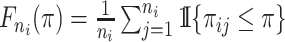be the empirical cumulative density function for the infectors of case , where is the number of possible infectors of case . Then counts the number of infectors with probability less than . The kernel density estimate at would be given by

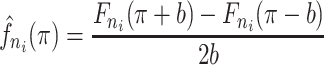(2.7)

where is the binwidth parameter. If for any within the range of the probabilities, then the high probability cluster of infectors is defined as all infectors with greater than the lowest value for which 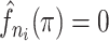. The bottom row of Figure 1 shows the kernel density estimates for the two example cases. With this clustering method, the generation interval estimate would depend in the binwidth, so like with hierarchical clustering, we average the results across multiple binwidths taken at regular intervals across the range of reasonable values.

2.5. Full estimation procedure

The steps to estimate the transmission interval using the modified PEM algorithm are as follows:

• 1. Estimate the relative probability of transmission between all pairs of cases () using naive Bayes (Leavitt and others, 2020) (do not use time between cases as a covariate).

• 2. Use hierarchical clustering or kernel density estimation to find the high probability clusters of infectors and determine if there is one for each case.

• 3. Estimate the transmission interval distribution parameters using the PEM algorithm only including the high probability cluster of infectors.

• 4. Calculate the mean, median, and standard deviation of the transmission interval distribution using the estimated parameters.

We also estimate confidence intervals for the summary statistics (mean, median, standard deviation) using cluster bootstrapping (Field and Welsh, 2007) where a cluster is all possible infectors for a given case. We sample cases with replacement with all of their possible infectors. We then repeat steps 3–4 with this bootstrap sample. After 1000 repetitions, we estimate the confidence intervals: and where is the mean, median, or standard deviation estimate of the transmission interval distribution and is the quantile function of the bootstrap estimates of . This modified PEM algorithm has been implemented in the R package nbTransmission v1.1.1 (Leavitt and others, 2020).

3. Simulation study

3.1. Data generation

We assess the performance of this modified PEM method with noise reduction to estimate the generation interval distribution by applying it to simulated outbreaks. Because this is simulated data, we know the infection times which allows us to estimate the true generation interval. Using R v3.6.0 (R Core Team, 2019), for each scenario we simulate 1000 outbreaks and generate the phylogenetic trees for those outbreaks with the TransPhylo v1.2.3 package (Didelot and others, 2017) and simulate genetic sequences corresponding to the phylogenetic trees with the phagnorn package v2.5.5 (Schliep, 2011). This procedure was used in Stimson and others (2019) and Leavitt and others (2020) for a similar purpose. We then simulate four arbitrarily chosen covariates with different forms that are associated with transmission to varying degrees.

The TransPhylo package simulates an outbreak by starting with one case and generating a transmission tree of the outbreak using the reproductive number (negative binomial distribution), the generation interval (gamma distribution), and the effective population size times the pathogen generation time (). The simulated outbreak continues until it either dies out, runs for a user-specified period of time, or reaches a user-specified sample size. The phangorn package then simulates genetic sequences from the phylogenetic tree represented by the transmission tree using the mutation rate and a random (or user-specified) base sequence. For all scenarios, we set and use a random 3000 base-pair sequence to generate the pathogen genomes (for more detail see the supplementary material available at Biostatistics online).

3.2. Simulation scenarios

To assess how different outbreak characteristics affect generation interval estimation, we simulate nine different scenarios in which we vary the sample size, reproductive number, mutation rate of the pathogen genome, and generation interval variance (with fixed mean). We start with a baseline scenario and then individually increase and decrease each parameter within the range of expected values for major pathogens as described in Campbell and others (2018) (Supplementary Table S1 available at Biostatistics online). The table also describes the time allowed for the outbreak, the single-nucleotide polymorphism (SNP) cutoffs to define probable links and nonlinks when estimating naive Bayes transmission probabilities, and the initial generation interval parameters. Details of the derivation of these parameters are described in the supplementary material available at Biostatistics online. For all scenarios we estimate the probabilities using the same four covariates and do not include the time between cases in the model because it is included in the calculation of (Equation 2.5).

For each of the 1000 simulated outbreaks from the nine scenarios, we compare the generation interval distribution estimated using various methods:

• 1. SNP distance alone: we use all probable links as defined by pathogen WGS and estimate the generation interval with the simple likelihood (Equation 2.2).

• 2. PEM (unmodified): we use the PEM algorithm (Equations 2.5, 2.6) with the naive Bayes probabilities including all pairs of cases.

• 3. PEM with top N: we adapt the PEM algorithm, restricting to the top N infectors with the highest probabilities (varying N from 1 to 10 by 1 and averaging across all cutoffs).

• 4. PEM with hierarchical clustering: we adapt the PEM algorithm by restricting to the high probability cluster of infectors as defined by hierarchical clustering (varying the cutoff from 0 to 0.25 by 0.025 and averaging across all cutoffs except 0).

• 5. PEM with kernel density estimation: We adapt the PEM algorithm by restricting to the high probability cluster of infectors as defined by kernel density estimation (varying the binwidth from 0.01 to 0.1 by 0.01 and averaging across all binwidths).

For a given cutoff or binwidth, the generation interval is only estimated if there are at least 10 cases who had a high probability cluster of infectors. To assess performance, we calculate the bias for each method by taking the difference between the mean, median, and standard deviation of the estimated generation interval and the values of these parameters for true pairs in that simulated outbreak. We summarize the bias over all outbreaks by calculating the mean absolute percentage error (MAPE): the average of the absolute value of the relative bias across all of the runs for each scenario. We calculated coverage—the percentage of confidence intervals which contained the true values of the mean, median, and standard deviation for the baseline scenario. We also assess the performance of the naive Bayes transmission probabilities to differentiate between truly linked and unlinked pairs by calculating the area under the receiver operating curve and determining what proportion of time the true infector was assigned the highest probability, or was ranked in the top 5%, 10%, 25%, and 50% of all possible infectors.

3.3. Simulation results

Figure 2 displays violin plots of the relative bias across the 1000 simulations for each scenario using the various methods for estimating the generation interval. For the top N, hierarchical clustering, and kernel density estimation, the results are for the averaged estimate over all cutoffs. We found that assuming that all pairs closer than a certain SNP distance are linked greatly overestimated the mean, median, and standard deviation of the generation interval. On the other hand, using the PEM algorithm including all pairs of cases underestimated these values.

Fig. 2.

Violin plots of the absolute bias in days for the mean (dark grey), median (medium grey), and standard deviation (light grey) of the generation interval distribution estimated by various methods for the nine different simulation scenarios: baseline, low, and high sample sizes (LowN, HighN), low and high reproductive numbers (LowR, HighR), low and high mutation rates (LowMR, HighMR), and low and high generation interval variances (LowGIV, HighGIV), described in detail in Supplementary Table 1 available at Biostatistics online. The absolute bias equals the observed value minus the true value and is in days. For PEM: top N, PEM: Hierarchical, and PEM: Kernel Density, the pooled results are shown. For the SNP distance method, but no other method the bias estimates for multiple scenarios extend above 10 days (the upper limit for this plot) to as high as 33 days. The plot is truncated here in order to better visualize the results of the other estimation methods.

All of the noise reduction methods greatly reduced the bias of the estimate, though using the top N pairs did not as consistently eliminate the bias as did using the high probability cluster of infectors identified by hierarchical clustering or kernel density estimation. Supplementary Figures S1–S3 available at Biostatistics online show the results for all of individual cutoffs for the three noise reduction methods and how these estimates compare to the pooled estimate shown in Figure 2. For hierarchical clustering and kernel density estimation, the bias was relatively constant across all cutoffs while for the top N, it was highly variable. Supplementary Figure S3 available at Biostatistics online also shows that if no cutoff is used for hierarchical clustering, the results have higher bias with more variability than all of the cutoffs suggesting it is important to exclude cases without a clear high probability cluster.

Across all of the scenarios, the pooled estimate had close to the same MAPE as the best performing cutoff/binwidth (Supplementary Figure S4 available at Biostatistics online). Additionally, except the scenarios with a low mutation rate or low sample size, the MAPE for the mean was 10% or less. When assessing the performance of the naive Bayes transmission probabilities, these scenarios also had the poorest performance across all metrics (Supplementary Figure S5 available at Biostatistics online). The MAPE for the standard deviation was higher than the MAPE for the mean and median across all scenarios, especially when the variance of the true generation interval differed from the baseline value with fixed mean. Our method overestimated the standard deviation when the variance was low (lower coefficient of variation) and underestimated the standard deviation when the variance was high (higher coefficient of variation). Therefore, although the mean of the generation interval was well estimated across all scenarios, the accuracy of the estimate of the median was more varied (Figure 2 and Supplementary Figure S4 available at Biostatistics online). We found that the coverage did not reach 95% (ranging between 80% and 90%) because though our estimates improved upon the unmodified PEM algorithm, they could not completely overcome the bias (Supplementary Figure S6 available at Biostatistics online).

4. Application to tuberculosis surveillance data

4.1. Description of data

We apply our methods to Massachusetts TB surveillance data for 2010–2016. The Department of Public Health (DPH) in Massachusetts, United States maintains a surveillance system of all active TB cases in the state including demographic, clinical, and pathogen genotyping data. During this time period, genotyping of all microbiologically-confirmed TB was routinely done using spacer oligonucelotide typing (spoligotype) and mycobacterial interspersed repetitive units variable number tandem repeats (MIRU-VNTR; 24 loci). For most cases, the TB lineage (L4—Euro-American, L1—Indo-Oceanic, L2—East Asian, L3—East African-Indian, or L6—West AfricanII) was also determined (Wiens and others, 2018). From the spoligotype and MIRU-VNTR patterns, the United States Center for Disease Control and Prevention (CDC) assigned a genotype group called a GENType for each case (Centers for Disease Control and Prevention, 2012). Contact investigations were done for many of these TB cases to evaluate contacts for TB disease, and identify any unrecognized links with previously detected TB cases.

4.2. Details of method application

We first define the observation date of each case as the earlier of two dates: the 15th of the month the case was first thought to have TB and the 15th of month the case was counted in the surveillance database (assuming the midpoint of the month since we do not have the exact date) as a proxy for symptom onset. We then apply the naive Bayes transmission method to obtain transmission probabilities for all ordered case-pairs who do not have different TB lineages, using GENType, sex, age, country of birth, county of residence, smear result, immune-suppression status, shared drug resistance as covariates. If cases were observed in the same month both orders of infector/infectee pairs are included.

We train the model using the subset of cases who were involved in a contact investigation. The probable links are cases who were found to be directly linked through contact investigation or cases who could both be linked to a common contact. The probable nonlinks are defined as pairs of cases who were both involved in contact investigations but were not linked to each other. When creating the training dataset, we only include unlinked pairs from a random subset of all cases who were involved in a contact investigation so that the number of cases included is consistent over time. For training pairs that were observed in the same month, the ordering was randomly chosen at each iteration of the naive Bayes transmission method.

We estimate the mean, median, and standard deviation of the serial interval distribution using the modified PEM algorithm described above with 95% bootstrap confidence intervals, clustering the infectors using both hierarchical clustering (varying cutoffs between 0.025 and 0.25 by 0.025 and averaging) and kernel density estimation (varying binwidths between 0.01 and 0.1 by 0.01 and averaging). The observed serial intervals are defined as the number of months between the observed dates of each pair. Therefore, cases observed in the same month are excluded because the time between them is unknown. We compare the estimated serial interval distribution using (i) an unmodified gamma distribution with no restriction on the serial interval, (ii) a shifted gamma distribution forcing the serial interval to be greater than 1 month ( = 1 month), or (iii) a shifted gamma distribution forcing the serial interval to be greater than 2 months ( = 2 months).

We also estimate the effective monthly reproductive number and average effective reproductive number for this time frame from the naive Bayes transmission probabilities using the method described in Leavitt and others (2020) which is independent of the estimated serial interval. For this analysis, we re-estimate the naive Bayes transmission probabilities including a categorical representation of the time between observed dates for the two cases. When estimating both the serial interval distribution and reproductive number we account for likely imported cases by setting the transmission probabilities to zero for all pairs where the infectee arrived in the United States less than 2 years before their observed date (unless the pair was linked by contact tracing) assuming that they were infected outside the country. As a sensitivity analysis, we also estimated both parameters using a 1 year instead of a 2-year window to define recent arrival.

4.3. Massachusetts TB results

There were 950 active TB cases (excluding five cases with M. bovis) diagnosed in Massachusetts and identified by the DPH between 2010 and 2016 (Supplementary Figure S7 available at Biostatistics online); 542 (57%) were men, 825 (87%) were not US-born, and 240 (28%) arrived in the United States within 2 years of being identified. TB lineage was known for most cases (92%) with more than half having lineage 4 (Euro-American). Additionally, all but five cases were assigned to a GENType (Supplementary Table S2 available at Biostatistics online). The 950 cases created 220 758 possible transmission pairs after excluding pairs where the possible infector was observed after the infectee and pairs with different lineages. The individual-level covariates were transformed into pair-level covariates as described in Table 2. Among the 950 cases, 35 could be connected through contact investigations to at least one other case in this time frame. From these cases and a random selection of cases who were involved in contact investigations but not connected to other cases, 26 probable linked pairs and 2058 probable nonlinked pairs were used to train the model. Supplementary Figure S8 available at Biostatistics online shows a histogram of the estimated probabilities for all pairs. The vast majority of these probabilities were extremely low, but there were pairs with high transmission probabilities indicating possible transmission events.

Table 2.

Pair-level equivalents of demographic and clinical characteristics for Massachusetts TB surveillance data from 2010 to 2016

Covariate	Level	N (%) of all Pairs
		(n = 220 578)
Sex	Male to male	71 170 (32.4)
	Female to female	41 097 (18.7)
	Male to female	51 067 (23.2)
	Female to male	56 602 (25.7)
Age group	Different	158 125 (71.6)
	Same	62 633 (28.4)
Country of birth	Different foreign country	147 618 (67.2)
	One United States, one foreign country	55 448 (25.2)
	Same foreign country	11 373 (5.2)
	Both United States born	5350 (2.4)
Smear result	Infector smear	89 364 (43.3)
	Infector smear+	117 055 (56.7)
Immune-suppression	Infector not suppressed	158 188 (71.7)
	Infector suppressed	62 570 (28.3)
Shared drug	Both drug susceptible	157 469 (71.3)
resistance	No shared resistance	59 005 (26.7)
	Shared resistance to 1 drug	3607 (1.6)
	Shared resistance to 2 drugs	569 (0.3)
	Shared resistance to 3+ drugs	108 (0.07)
County of	Same county	40 524 (18.4)
residence	Neighboring counties	98 082 (44.5)
	More distant counties	81 919 (37.1)
CDC GENType†	Not matching	215 610 (99.8)
	Matching	363 (0.2)
Time between	1 year	60 762 (27.5)
observed dates	1–2 years	47 722 (21.6)
	2–3 years	39 416 (17.9)
	3–4 years	30 803 (14.0)
	4+ years	42 055 (19.1)

^†Defined as matching on spoligotype and all 24 MIRU-VNTR loci

With an unmodified gamma, our estimated serial interval distribution had mean of 1.33 years (95% confidence interval [CI] 1.19–1.46) and standard deviation of 1.33 years (95% CI: 1.17–1.48) using the hierarchical clustering pooled estimate. The estimate using kernel density estimation was very similar (mean: 1.28 years [95% CI: 1.13–1.44], standard deviation: 1.29 years [95% CI: 1.13–1.46]). Forcing the distribution to be more than 1 month, the estimated mean was 1.47 (95% CI: 1.31–1.60) with hierarchical clustering and 1.42 (95% CI: 1.25–1.57) with kernel density estimation. Forcing the distribution to be more than 2 months, the estimated mean was 1.58 (95% CI: 1.42–1.73) with hierarchical clustering and 1.54 (95% CI: 1.36–1.70) with kernel density estimation. The standard deviation estimates were similar across all three exclusion criteria. The median estimates were notably lower than the mean for all methods, but followed the same patterns as described above for the mean. The estimates were fairly consistent across the different methods and cutoffs. The range of mean estimates across the different cutoffs was 1.23–1.48 years when no there was no restriction on the serial interval, 1.35–1.61 years with serial intervals greater than a month, and 1.46–1.70 years with serial intervals greater than 2 months (Figure 3 and Supplementary Tables S3 and S4 available at Biostatistics online).

Fig. 3.

Estimates of the mean, median, and standard deviation for the serial interval of TB in Massachusetts between 2010 and 2016 estimated from relative transmission probabilities with 95% bootstrap confidence intervals. The left panels shows the results when clustering the infectors using hierarchical clustering with various cutoffs and the right panels with kernel density estimation with various binwidths. The solid horizontal lines show the pooled estimates (averaging over all cutoffs/binwidths) with their 95% confidence intervals as dotted lines. The blue lines show the estimates from an unmodified gamma distribution with no restriction on the serial interval, the green using a shifted gamma distribution forcing the serial interval to be greater than 1 month and the red using a shifted gamma distribution forcing the serial interval to be greater than 2 months.

Finally, we estimated the monthly effective reproductive number for TB in this context depicted in Supplementary Figure S9 available at Biostatistics online. Importantly, these estimates account for imported cases from recent immigration by assuming that recent immigrants were not infected by the sampled cases. By averaging the monthly effective reproductive numbers, we estimate that the overall effective reproductive number for TB in Massachusetts is 0.77 (95% CI 0.71–0.84). We found that changing the definition of recent arrival to the United States from 2 years to 1 year had a negligible effect of both the serial interval and reproductive number estimates (Supplementary Figures S10 and S11 available at Biostatistics online).

5. Discussion

We developed a method to estimate transmission intervals using outbreak or surveillance data with limited WGS and/or contact investigation data which extends the PEM algorithm developed by Hens and others (2012) to incorporate naive Bayes transmission probabilities. We showed that our method can more accurately estimate the generation interval in simulations of various outbreak characteristics than the PEM algorithm without modification or assuming that presumed linked cases (with fewer than a certain number of SNPs) are truly linked.

Our modification uses various methods to cluster the possible infectors for each cases identifying the few most likely infectors. Clustering using hierarchical clustering and kernel density estimation resulted in fairly consistent estimates across multiple cutoffs or binwidths and the pooled estimate had close to the lowest error in all scenarios. However, the simpler method of including the top N infectors with the highest probability had highly variable results depending on the choice of N, making the other two methods preferable. Using any of the three methods greatly decreased the bias that resulted when using the unmodified PEM algorithm in this context.

We applied the modified PEM algorithm to estimate the TB serial interval in Massachusetts between 2010 and 2016. The estimated mean of the generation interval distribution was around 1.3 years (SD: 1.3) with an unmodified gamma distribution and 1.5 years (SD: 1.4) when forcing the serial interval to be more than 2 months. We found that the estimates were consistent between the various cutoffs for the two different methods, varying by less than 2 months, except for a few outliers. There have been few published serial interval estimates for TB, but most studies also estimated the mean serial interval to be between 1 and 2 years depending on the location, study design, and method (Ma and others, 2018; Didelot and others, 2017; Leung and others, 2013; ten Asbroek and others, 1999; Borgdorff and others, 2011; Brooks-Pollock and others, 2011; Ma and others, 2020). We also estimated the overall monthly reproductive number for Massachusetts to be 0.77 when accounting for likely imported cases.

In our simulations results, we found that the generation interval estimate was sensitive to various factors. The accuracy depends on how well the probabilities estimated using naive Bayes can differentiate between linked and unlinked pairs. This probability performance is affected by the training dataset size, accuracy of WGS or contact investigations to identify links, and how informative the covariates are in identifying transmission. Using confirmed contact as in the TB application ensures that the probable links have interacted, but may miss links with unknown or unreported contacts. The estimation of these probabilities could be affected by incomplete and/or biased sampling particularly by a biased training dataset. Our Massachusetts TB results could also have been affected by the very low number of confirmed contacts that were found and used to train the model. A small training dataset is less likely to represent the true distribution of covariates for transmission pairs than a larger training dataset. Our results could also be biased if undetected cases had different serial intervals than detected cases. Additionally, any simulated mutation process simplifies reality, which could affect our simulation results. These limitations also apply to the reproductive number estimate as described in Leavitt and others (2020).

The true coefficient of variation of the generation interval (the ratio between the standard deviation and the mean) also affected the accuracy of the estimation of the standard deviation of the distribution. The coefficient of variation was identified in Griffin and others (2011) as impacting the joint estimation of the generation interval and reproductive number which is indirectly what our method is doing. We found that the noise of the distribution of the time between all pairs of cases prevented the unmodified PEM algorithm from accurately estimating the generation interval distribution. This noise is perhaps the reason that even the modified PEM algorithm had difficulty estimating the standard deviation in certain contexts. If the true generation interval shape (which is affected by the coefficient of variation) is far different than this underlying noise distribution, then it is more difficult to overcome that noise.

We found that the confidence interval coverage was lower than desired especially for the standard deviation. This is an important limitation of our work that reflects the difficulty of estimating transmission intervals in any context. Although we were able to shrink the bias of the unmodified PEM algorithm, there is still uncertainty in determining infector-infectee pairs or noise introduced by unlinked pairs creating bias in estimates meaning that we do not achieve 95% coverage. However, we show that the bias is minimal, and the results resemble truth.

All methods to estimate transmission intervals have to deal with uncertainty surrounding the date of infection or symptom onset. In simulations, we used the true infection date, a best-case scenario. In most applications, we do not know the infection date and or even the symptom onset date. In our Massachusetts analysis, we used the earlier of the date the case was first identified and the date they were counted in the dataset as a proxy for symptom onset. Therefore, though we call this estimate the serial interval to be consistent with other literature, our estimate could be more accurately described as an observation interval. Others have noted that the relationship between the serial and generation intervals is complicated and depends on the outbreak setting (Svensson, 2007; Pavlin, 2014; Britton and Tomba, 2019). This difference between the intervals is important when using the estimated serial interval to estimate other outbreak characteristics. Additionally, we do not always know the order of infection for some pairs of cases resulting in the possibility of negative serial intervals. This is especially true when analyzing TB outbreaks due to the long time between infection and symptom onset and non-specificity of the symptoms.

Here, we use a simple underlying likelihood to describe the transmission interval which, though it can account for co-prevalent cases, does not account for censoring or other considerations. However, the estimation framework that we outlined here - using the PEM algorithm with clustering of infectors—could easily be adapted to use a more complex likelihood such as the cure model method developed by Ma and others (2020). Also, the transmission probabilities could be estimated with other methods, such as Didelot and others (2017) or Worby and others (2014), which use complete WGS data. Finally, our noise reduction method of finding the high probability cluster of infectors could be used in other applications when considering all possible pairs of cases leads to noise overwhelming the signal.

Transmission interval estimates are rare for many diseases despite their importance in understanding outbreak dynamics because these intervals are difficult to estimate without knowing who infected whom. Additionally, methods that exist to estimate these intervals rely on specific types of data: household contacts, pathogen WGS data, etc. which limit their applicability to many rich existing outbreak datasets. We have shown how routine surveillance data can be used to estimate transmission intervals using a novel method that incorporates different sources of information and does not rely on complete WGS data or contact tracing data. The method we developed provides yet another tool to help to unravel this illusive and important outbreak characteristic.

6. Software

The methods developed here are implemented in the R package nbTransmission which is available on CRAN and GitHub at https://github.com/sarahleavitt/nbTransmission (DOI: 10.5281/zenodo.3952553). The code used to produce all results reported in this article is also available on GitHub at https://github.com/sarahleavitt/nbSimulation (DOI: 10.5281/zenodo.3676048) and https://github.com/sarahleavitt/nbPaper2 (DOI: 10.5281/zenodo.3667805).

Supplementary material

Supplementary material is available at http://biostatistics.oxfordjournals.org.

Funding

This work was supported by the US National Institutes of Health (NIH) [NIHGMS R01GM122876]. S.V.L. was also funded by the Interdisciplinary Training grant from the US NIH [NIHGMS T32GM074905]. H.E.J. was also funded by US NIH [NIH K01AI102944]. C.R.H. and L.F.W. were also funded by the Providence/Boston Center for AIDS Research [P30AI042853]. C.R.H. was supported by the Boston University/Rutgers Tuberculosis Research Unit [U19AI111276] and the US-India Vaccine Action Program (VAP) Initiative on Tuberculosis (CRDF Global/NIAID). R.S.L. holds a Fellowship from the Canadian Institutes of Health Research [MFE-152448]. The content of the article is solely the responsibility of the authors and does not necessarily represent the views of the National Institute of Allergy and Infectious Disease or the Office of the Director, NIH. The funders had no role in the decision to publish this article.

References

- Becker, N. G., Wang, D. and Clements, M. (2010). Type and quantity of data needed for an early estimate of transmissibility when an infectious disease emerges. Eurosurveillance 15, 1–6. [PubMed] [Google Scholar]
- Borgdorff, M. W., Sebek, M., Geskus, R. B., Kremer, K., Kalisvaart, N. and van Soolingen, D. (2011). The incubation period distribution of tuberculosis estimated with a molecular epidemiological approach. International Journal of Epidemiology 40, 964–970. [DOI] [PubMed] [Google Scholar]
- Britton, T. and Tomba, G. S. (2019). Estimation in emerging epidemics: biases and remedies. Journal of the Royal Society Interface 16, 1–10. [DOI] [PMC free article] [PubMed] [Google Scholar]
- Brooks-Pollock, E., Becerra, M. C., Goldstein, E., Cohen, T. and Murray, M. B. (2011). Epidemiologic inference from the distribution of tuberculosis cases in households in Lima, Peru. The Journal of Infectious Diseases 203, 1582–1589. [DOI] [PMC free article] [PubMed] [Google Scholar]
- Campbell, F., Cori, A., Ferguson, N., Baker, S. and Jombart, T. (2019). Bayesian inference of transmission chains using timing of symptoms, pathogen genomes and contact data. PLoS Computational Biology 15, 1–20. [DOI] [PMC free article] [PubMed] [Google Scholar]
- Campbell, F., Strang, C., Ferguson, N., Cori, A. and Jombart, T. (2018). When are pathogen genome sequences informative of transmission events? PLoS Pathogens 14, 1–21. [DOI] [PMC free article] [PubMed] [Google Scholar]
- Cauchemez, S., Boëlle, P.-Y., Donnelly, C. A., Ferguson, N. M., Thomas, G., Leung, G. M., Hedley, A. J., Anderson, R. M. and Valleron, A.-J. (2006). Real-time estimates in early detection of SARS. Emerging Infectious Diseases 12, 110–113. [DOI] [PMC free article] [PubMed] [Google Scholar]
- Centers for Disease Control and Prevention. (2012). GENType: new genotyping terminology to intergrate 24-locus MIRU-VNTR. Technical Report, Centers for Disease Control and Prevention, Atlanta, Georgia. [Google Scholar]
- Champredon, D. and Dushoff, J. (2015). Intrinsic and realized generation intervals in infectious-disease transmission. Proceedings of the Royal Society B: Biological Sciences 282, 1–10. [DOI] [PMC free article] [PubMed] [Google Scholar]
- Cowling, B. J., Fang, V. J., Riley, S., Peiris, J. S. M. and Leung, G. M. (2009). Estimation of the serial interval of influenza. Epidemiology 20, 344–347. [DOI] [PMC free article] [PubMed] [Google Scholar]
- Didelot, X., Fraser, C., Gardy, J. and Colijn, C. (2017). Genomic infectious disease epidemiology in partially sampled and ongoing outbreaks. Molecular Biology and Evolution 34, 997–1007. [DOI] [PMC free article] [PubMed] [Google Scholar]
- Field, C. A. and Welsh, A. H. (2007). Bootstrapping clustered data. Journal of the Royal Statistical Society. Series B: Statistical Methodology 69, 369–390. [Google Scholar]
- Griffin, J. T., Garske, T., Ghani, A. C. and Clarke, P. S. (2011). Joint estimation of the basic reproduction number and generation time parameters for infectious disease outbreaks. Biostatistics 12, 303–312. [DOI] [PubMed] [Google Scholar]
- Hall, M., Woolhouse, M. and Rambaut, A. (2015). Epidemic reconstruction in a phylogenetics framework: transmission trees as partitions of the node set. PLoS Computational Biology 11, 1–36. [DOI] [PMC free article] [PubMed] [Google Scholar]
- Hens, N., Calatayud, L., Kurkela, S., Tamme, T. and Wallinga, J. (2012). Practice of epidemiology robust reconstruction and analysis of outbreak data: influenza A(H1N1)v transmission in a school-based population. American Journal of Epidemiology 176, 196–203. [DOI] [PubMed] [Google Scholar]
- Jombart, T., Cori, A., Didelot, X., Cauchemez, S., Fraser, C. and Ferguson, N. (2014). Bayesian reconstruction of disease outbreaks by combining epidemiologic and genomic data. PLoS Computational Biology 10, 1–14. [DOI] [PMC free article] [PubMed] [Google Scholar]
- Klinkenberg, D., Backer, J. A., Didelot, X., Colijn, C. and Wallinga, J. (2017). Simultaneous inference of phylogenetic and transmission trees in infectious disease outbreaks. PLoS Computational Biology 13, 1–32. [DOI] [PMC free article] [PubMed] [Google Scholar]
- Leavitt, S. V., Lee, R. S., Sebastiani, P., Horsburgh, Jr, C. R., Jenkins, H. E. and White, L. F. (2020). Estimating the relative probability of direct transmission between infectious disease patients. International Journal of Epidemiology, 49, 764–775. [DOI] [PMC free article] [PubMed] [Google Scholar]
- Leung, E. C. C., Leung, C. C., Kam, K. M., Yew, W. W., Chang, K. C., Leung, W. M. and Tam, C. M. (2013). Transmission of multidrug-resistant and extensively drug-resistant tuberculosis in a metropolitan city. European Respiratory Journal 41, 901–908. [DOI] [PubMed] [Google Scholar]
- Ma, Y., Horsburgh, Jr, C. R., White, L. F. and Jenkins, H. E. (2018). Quantifying TB transmission: a systematic review of reproductive number and serial interval estimates for tuberculosis. Epidemiology and Infection 146, 1478–1494. [DOI] [PMC free article] [PubMed] [Google Scholar]
- Ma, Y., Jenkins, H. E., Sebastiani, P., Ellner, J. J., Jones-López, E. C., Dietze, R., Horsburgh, Jr, C. R. and White, L. F. (2020). Using cure models to estimate the serial interval of tuberculosis with limited follow-up. American Journal of Epidemiology, 189, 764–775. [DOI] [PMC free article] [PubMed] [Google Scholar]
- Moser, C. B., Gupta, M., Archer, B. N. and White, L. F. (2015). The impact of prior information on estimates of disease transmissibility using Bayesian tools. PLoS One 10, 1–16. [DOI] [PMC free article] [PubMed] [Google Scholar]
- Murtagh, F. and Contreras, P. (2012). Algorithms for hierarchical clustering: an overview. Wiley Interdisciplinary Reviews: Data Mining and Knowledge Discovery 2, 86–97. [Google Scholar]
- Park, S. W., Champredon, D., Weitz, J. S. and Dushoff, J. (2019). A practical generation-interval-based approach to inferring the strength of epidemics from their speed. Epidemics 27, 12–18. [DOI] [PubMed] [Google Scholar]
- Pavlin, B. I. (2014). Calculation of incubation period and serial interval from multiple outbreaks of Marburg virus disease. BMC Research Notes 7, 1–6. [DOI] [PMC free article] [PubMed] [Google Scholar]
- R Core Team. (2019). R: A language and environment for statistical computing. R Foundation for Statistical Computing, Vienna, Austria. https://www.R-project.org/. [Google Scholar]
- Schliep, K. P. (2011). phangorn: phylogenetic analysis in R. Bioinformatics 27, 592–593. [DOI] [PMC free article] [PubMed] [Google Scholar]
- Stimson, J., Gardy, J., Mathema, B., Crudu, V., Cohen, T. and Colijn, C. (2019). Beyond the SNP threshold: identifying outbreak clusters using inferred transmissions. Molecular Biology and Evolution 36, 587–603. [DOI] [PMC free article] [PubMed] [Google Scholar]
- Svensson, A. (2007). A note on generation times in epidemic models. Mathematical Biosciences 208, 300–311. [DOI] [PubMed] [Google Scholar]
- ten Asbroek, A. H. A., Borgdorff, M. W., Nagelkerke, N. J. D., Sebek, M. M. G. G., Deville, W., van Embden, J. D. A. and van Soolingen, D. (1999). Estimation of serial interval and incubation period of tuberculosis using DNA fingerprinting. International Journal of Tuberculosis and Lung Disease 3, 414–420. [PubMed] [Google Scholar]
- Vink, M. A., Christoffel, M., Bootsma, J. and Wallinga, J. (2014). Systematic reviews and meta- and pooled analyses serial intervals of respiratory infectious diseases: a systematic review and analysis. American Journal of Epidemiology 180, 865–875. [DOI] [PubMed] [Google Scholar]
- Wallinga, J. and Teunis, P. (2004). Different epidemic curves for severe acute respiratory syndrome reveal similar impacts of control measures. American Journal of Epidemiology 160, 509–516. [DOI] [PMC free article] [PubMed] [Google Scholar]
- White, L. F. and Pagano, M. (2008). A likelihood-based method for real-time estimation of the serial interval and reproductive number of an epidemic. Statistics in Medicine 27, 2999–3016. [DOI] [PMC free article] [PubMed] [Google Scholar]
- Wiens, K. E., Woyczynski, L. P., Ledesma, J. R., Ross, J. M., Zenteno-Cuevas, R., Goodridge, A., Ullah, I., Mathema, B., Djoba S., Joel Fleury, B., Molly H., Ray, S. E., Bhattacharjee, N. V., Henry, N. J., Reiner, R. C., Kyu, H. H., Murray, C. J. L.. and others. (2018). Global variation in bacterial strains that cause tuberculosis disease: a systematic review and meta-analysis. BMC Medicine 16, 1–13. [DOI] [PMC free article] [PubMed] [Google Scholar]
- Worby, C. J., Chang, H.-H., Hanage, W. P. and Lipsitch, M. (2014). The distribution of pairwise genetic distances: a tool for investigating disease transmission. Genetics 198, 1395–1404. [DOI] [PMC free article] [PubMed] [Google Scholar]
Associated Data
This section collects any data citations, data availability statements, or supplementary materials included in this article.