Geographically weighted generalized Farrington algorithm for rapid outbreak detection over short data accumulation periods

Abstract

The demand for rapid surveillance and early detection of local outbreaks has been growing recently. The rapid surveillance can select timely and appropriate interventions toward controlling the spread of emerging infectious diseases, such as the coronavirus disease 2019 (COVID‐19). The Farrington algorithm was originally proposed by Farrington et al (1996), extended by Noufaily et al (2012), and is commonly used to estimate excess death. However, one of the major challenges in implementing this algorithm is the lack of historical information required to train it, especially for emerging diseases. Without sufficient training data the estimation/prediction accuracy of this algorithm can suffer leading to poor outbreak detection. We propose a new statistical algorithm—the geographically weighted generalized Farrington (GWGF) algorithm—by incorporating both geographically varying and geographically invariant covariates, as well as geographical information to analyze time series count data sampled from a spatially correlated process for estimating excess death. The algorithm is a type of local quasi‐likelihood‐based regression with geographical weights and is designed to achieve a stable detection of outbreaks even when the number of time points is small. We validate the outbreak detection performance by using extensive numerical experiments and real‐data analysis in Japan during COVID‐19 pandemic. We show that the GWGF algorithm succeeds in improving recall without reducing the level of precision compared with the conventional Farrington algorithm.

1. INTRODUCTION

The demand for statistical surveillance systems has increased in recent decades. It was driven not only by globalization, disasters, and terrorism but also by emerging infectious diseases, such as SARS, MERS, swine flu, and the coronavirus disease 2019 (COVID‐19), as well as the persistent public health issues related to infectious disease outbreaks. It is important to rapidly survey and expeditiously detect local outbreaks. The rapid surveillance can select timely and appropriate interventions toward controlling the spread of the disease. Numerous statistical methods have been proposed on this topic, inspired by a wide range of conventional/recent statistical techniques: for example, autoregressive‐based regression for modeling time trend, scan statistics approach for hotspots detection, and point process‐based models for breakpoints detection on time series data. The detailed literature reviews of the development can be found elsewhere. ¹ , ² , ³ , ⁴ , ⁵

To tackle an emerging infectious disease pandemic, it is common to estimate and monitor a rapid increase in mortality that is greater than expected under normal circumstances (ie, under the counterfactual situation without the pandemic). It assesses the mortality burden of the new pandemic, the so‐called “excess death” approach. ⁶ , ⁷ Regarding the COVID‐19 pandemic, several methods for estimating excess death have been proposed to quantify the formal underestimation of the COVID‐19 mortality burden in many heavily affected countries. ⁸ , ⁹ , ¹⁰ , ¹¹ For example, there are two popular algorithms, that is, FluMOMO and Farrington, that are frequently used in practice. European mortality monitoring activity (EuroMOMO), which is supported by the European Center for Disease Prevention and Control and the World Health Organization, adopted the FluMOMO algorithm by using official national mortality statistics provided weekly from the 27 European countries in the EuroMOMO network. ¹² The algorithm is based on a simple, yet robust quasi‐Poisson regression model with several nonlinear terms for seasonality and influenza activity, and it has been widely used, especially in European countries. ¹³ , ¹⁴ The Farrington algorithm ⁶ , ⁷ is commonly used to estimate excess death by the United States Centers for Disease Control and Prevention (CDC), which updates the estimates weekly and supports the decision‐making process for the control of COVID‐19 in the United States. ¹⁵ The algorithm is also based on a quasi‐Poisson regression model, which will be explained subsequently, and has been extensively used in many countries to estimate the country‐specific excess death related to COVID‐19 in a timely manner. ¹⁶ , ¹⁷ , ¹⁸ Noufaily et al ⁷ extended the Farrington algorithm by incorporating robust residuals and conducted extensive simulation experiments for improving the specificity, whose generalization is our interest in this study. Reviews of other outbreak detection methods using time series data can be found in Buckeridge, ¹⁹ Unkel et al, ² and Noufaily et al. ²⁰

One of the major challenges currently facing large outbreak detection survey systems is that long‐term data are sometimes unavailable. Thus, the number of time points is insufficient and the estimation/prediction accuracy is poor, resulting in a worse outbreak detection performance. To address this issue, we propose a new statistical algorithm—the geographically weighted generalized Farrington (GWGF) algorithm—to analyze time series count data sampled from a spatially correlated process for estimating excess death. In general, the use of the geographical neighborhood information enables the stabilization of the estimation by improving the estimation efficiency at the expense of bias. ²¹ , ²² , ²³ , ²⁴ Using this property, our method is designed to achieve a stable detection of outbreaks even when the number of time points is small. This technique is especially useful in surveying emerging diseases for which minimal data have been accumulated. It is also beneficial in areas where a surveillance system is under development such that historical data have not been accumulated. In this study, as with Nakaya et al ²⁵ who proposed the geographically weighted Poisson regression, we propose an algorithm that utilizes geographically weighted regression techniques with spatial kernels and a quasi‐likelihood approach, including the quasi‐Poisson regression model. By assigning geographical weights, which correspond to the distance among the observation's locations, to each observation, the local quasi‐likelihood model is constructed.

In this article, we revisit the current Farrington algorithm and its extension by Noufaily et al ⁷ with a view to improve its detection performance under the insufficient time series data scenario. Furthermore, we propose our approach, the GWGF algorithm, by using a local quasi‐likelihood regression model with geographically induced weights. The detection performance of outbreaks is extensively examined in the simulation experiments and real‐world data in Sections 3 and 4. Lastly, we discuss the implications of our findings and limitations in Section 5.

2. METHOD

In this section, we first explain a popular algorithm for estimating the degree of excess death, that is, the Farrington algorithm, ⁶ , ⁷ and then extend the algorithm to a more flexible form by incorporating covariates and geographical information in a similar manner as proposed by Zhang et al, ²⁶ Brunsdon et al, ²⁷ and Fotheringham et al. ²¹

2.1. Current algorithm: Farrington algorithm

We first review the current Farrington algorithm proposed by Farrington et al ⁶ and extended by Noufaily et al. ⁷ Full details can be found in Noufaily et al. ⁷ Here, we explain the aspects of the algorithm to be possibly improved in the following sections.

Assume that we have T time points data ($t=1,\dots ,T$) and each t indicates time such as a week, month, or year. Let ${\{y_t\}}_{t=1}^T$ be a univariate time series of counts (ie, the number of death in the context of excess death analysis). At any week $t_c\ge 1$, the available information is the historical count ${\mathit{H}}_{t_c}=\{y_t;t\le t_c\}$. Excess death at a certain week $t_c$ is defined as

$$\begin{array}{ll}{N}_{t_c}=\max \{y_{t_c}-U,0\}& \end{array}$$ (1)

based on the known threshold value U with a resulting alarm defined as:

$$\begin{array}{ll}{A}_{t_c}=\left\{\begin{array}{c}1(\text{if}{y}_{t_c}>U),\\ 0\text{(otherwise)}.\end{array}\right.& \end{array}$$ (2)

In the context of the excess death analysis context, as described in the following section, U is frequently set to be the $100(1-\alpha )$‐percentile upper bound of the prediction distribution at time $t_c$.

In the first step, a quasi‐Poisson model with a log link function is fitted to the baseline data ${\mathit{H}}_t$, where $y_t$ is assumed to be distributed with mean ${\mu }_t$ and variance $\varphi {\mu }_t$ ($\varphi$ is called a dispersion parameter). Thus, it is modeled as

$$E[y_t]={\mu }_t=\exp (\alpha +\beta t),$$ (3)

and $\mathrm{Var}(y_t)=\varphi {\mu }_t$, where $\varphi \ge 1$ and $\alpha$ and $\beta$ are regression parameters that are frequently estimated by the quasi‐likelihood method.

In the original Farrington paper, ⁶ the subset of the baseline data ${\mathit{H}}_t$ is further specified by two parameters, b and w: b is the number of previous years to be considered and w is the (half) window size. The baseline data are extracted during $t-w$ and $t+w$ weeks of years $h-b$ to $h-1$, where h is the year of t, giving a total of $n=b(2w+1)$ baseline weeks in the baseline data at time t. Note that in Noufaily et al, ⁷ the linear trend term $\beta t$ can be dropped if it is nonsignificant at the 5% level or if ${\widehat{\mu }}_t>\max \{{\mathit{H}}_t\}$, where ${\widehat{\mu }}_t=\exp (\widehat{\alpha }+\widehat{\beta }t)$; however, our method does not employ this rule. Given ${\widehat{\mu }}_t$ where the estimated parameters $\widehat{\alpha }$ and $\widehat{\beta }$ are plugged into (3), the dispersion parameter $\varphi$ is estimated by

$$\begin{array}{lcr}\widehat{\varphi }=\max \left\{{\displaystyle \frac{1}{n-p}}{\displaystyle \sum _{t=1}^n}{\displaystyle \frac{v_t{(y_t-{\widehat{\mu }}_t)}^2}{{\widehat{\mu }}_t}},1\right\},& & \end{array}$$

where p is the number of covariates in the model (ie, $p=2$), $v_t$ is down weight that alleviates the bad effect of the past weeks with outlying counts to the baseline estimation and is estimated by Anscombe residuals, ⁷ , ²⁸ and ${\sum }_{i=t}^n{v}_t=1$.

Next step is to define the threshold U. Noufaily et al ⁷ use the following threshold value, which is approximated by the normal distribution after the $2/3$ power transformation for the correction in skewness of the Poisson distribution; ²⁹

$$\begin{array}{lcr}U={\widehat{\mu }}_{t_c}{\left\{1+{\displaystyle \frac{2}{3}}{z}_{1-\alpha }{\widehat{\mu }}_{t_c}^{-1}(\widehat{\varphi }{\widehat{\mu }}_{t_c}+\mathrm{Var}{({\widehat{\mu }}_{t_c})}^{1/2})\right\}}^{3/2},& & \end{array}$$

where $z_{1-\alpha }$ is the $100(1-\alpha )$‐percentile of the normal distribution.

This algorithm is easily implemented by using the R package surveillance ³⁰ with an overview at (http://surveillance.r‐forge.r‐project.org/). This algorithm has been successful in many areas, including the CDC in the United States to capture the excess death situation in a timely manner. However, the original algorithm does not allow us to include any covariates, and more importantly, the detection accuracy (such as the sensitivity and specificity of detecting outbreaks) is unstable, especially when the long‐term data are unavailable. This can happen frequently in the surveillance of emerging infectious diseases. To address them, we generalize the Farrington algorithm by extending model (3) to a more flexible form with other covariates, such as weekly temperature or the number of influenza cases per week. Moreover, we incorporate the spatial dependency between the locations within the area of interest to improve the estimation by borrowing the strength from the neighborhood locations, thereby resulting in stable outbreak detection.

2.2. Geographically weighted generalized Farrington algorithm

In this subsection, we generalize the original nonspatial Farrington algorithm to incorporate additional covariates and geographical dependency, which we refer to as the GWGF algorithm. Let ${\mathit{u}}_j=(u_{1j},u_{2j})\in {ℝ}^2$ be a two‐dimensional vector describing the geographical location (coordinates) of a location j ($j=1,\dots ,J$) and $y_{tj}$ be the count (ie, the weekly number of deaths) in week t at location j. The extended semi‐varying quasi‐Poisson model for the jth location is then defined as:

$$E[y_{tj}]={\mu }_{tj}=\exp ({\alpha }_j+{\beta }_{j}t+{\mathit{X}}_{tj}{\mathit{\gamma }}_j+{\mathit{Z}}_t\mathit{\zeta }+{\delta }_{jt}),$$ (4)

where ${\mathit{X}}_{tj}\in {ℝ}^{q_1}$ and ${\mathit{\gamma }}_j\in {ℝ}^{q_1}$ are a geographically varying covariate vector at time t and a geographically varying coefficient vector at the jth location, respectively; ${\mathit{Z}}_t\in {ℝ}^{q_2}$ and $\mathit{\zeta }\in {ℝ}^{q_2}$ are a geographically invariant covariate vector at time t and a geographically invariant coefficient vector, respectively; and ${\delta }_{jt}$ is a seasonal dummy variable corresponding to week t in the jth location, with $jt=0$ and ${\delta }_{0j}=0$, which means that the current week is always within the reference season. The dummy variable ${\delta }_{jt}$ is introduced by Noufaily et al ⁷ (cf. they called it the zeroth‐order spline) to account for the seasonality and they recommend the inclusion of 10‐levels factors with one 7‐week reference period (corresponding to week $t_c\pm 3$ weeks) and nine 5‐week periods each year.

As $\mathit{\zeta }$ is a constant vector, Equation (4) cannot be treated statistically as a special case of varying coefficient models such as Hastie and Tibshirani. ³¹ Zhang et al ²⁶ studied the semi‐varying coefficient model (4) and propose a two‐step estimation procedure. We briefly explain the steps, which are tailored to our case: the first step is to treat $\mathit{\zeta }$ as ${\mathit{\zeta }}_j$) and estimate it by using the following local quasi‐likelihood approach. Thereafter, we average ${\mathit{\zeta }}_j$ over $j=1,\dots ,J$ to get the final estimator of $\mathit{\zeta }$. Once $\mathit{\zeta }$ is estimated, the model (4) is reduced to a standard varying coefficient model: see Hastie and Tibshirani. ³¹ For simplicity, we assume $\mathit{\zeta }=0$ (thus drop the term ${\mathit{Z}}_t\mathit{\zeta }$ from Equation 4) in the following discussion.

To estimate the set of parameters ${\mathit{\theta }}_j={({\alpha }_j,{\beta }_j,{\mathit{\gamma }}_j^T)}^T$ in Equation (4), we employ the idea of local likelihood principal ²³ or equivalently, the geographically weighted likelihood principal. ²⁵ Based on the principal, to obtain the estimates of ${\mathit{\theta }}_j$, we extend the quasi‐likelihood estimating equation proposed by Wu (1996) ²² as:

$$L({\mathit{\theta }}_j)={\displaystyle \sum _{t=1}^n}\sum _{1\le j^{\prime }\ne j\le J}{w}_{j{j}^{\prime }}{\displaystyle \frac{y_{tj}-{\mu }_{tj}}{{\varphi }_j{\mu }_{tj}}}{\displaystyle \frac{\partial {\mu }_{tj}}{\partial {\mathit{\theta }}_j}}=\mathbf{0},$$ (5)

where $w_{j{j}^{\prime }}$ is a geographical weight at the location of j. It is a decreasing function of the distance between location ${\mathit{u}}_j$ and ${\mathit{u}}_{j^{\prime }}$. One classical choice of the spatial weighting function is a Gaussian kernel class defined as

$$\begin{array}{lcr}{w}_{j{j}^{\prime }}=\exp \left({\displaystyle \frac{-\Vert {\mathit{u}}_j-{\mathit{u}}_{j^{\prime }}{\Vert }^2}{{\sigma }_j^2}}\right),& & \end{array}$$

where ${\sigma }_j$, which is referred to as a bandwidth, controls the kernel size. $w_{j{j}^{\prime }}$ puts more weights on the locations in closer proximity and less weights on the location in remote proximity to the estimation for the location of j. Alternatively, it is also possible to use the adaptive approach that allows the inclusion of the same number of data points. The popular adaptive kernel is the bi‐square kernel, which is defined by

$$\begin{array}{lcr}{w}_{j{j}^{\prime }}=\left\{\begin{array}{cc}{\{1-{(\Vert {\mathit{u}}_j-{\mathit{u}}_{j^{\prime }}\Vert /{\sigma }_j^2)}^2\}}^2& \text{if}\Vert {\mathit{u}}_j-{\mathit{u}}_{j^{\prime }}\Vert <{\sigma }_j^2,\\ 0& \text{otherwise},\end{array}\right.& & \end{array}$$

where ${\sigma }_j$ controls the kernel size, which includes the Mth nearest locations from the location j. The number of locations M should be exogenously given by users. More detailed discussions on the choice of the geographical kernels can be found in Fotheringham et al. ²¹ By solving the estimating equation (5), we obtain the estimates ${\widehat{\mathit{\theta }}}_j={({\widehat{\alpha }}_j,{\widehat{\beta }}_j,{\widehat{\mathit{\gamma }}}_j^T)}^T$. According to the result of McCullagh, ³² the value of $\widehat{\mathit{\theta }}$ is not (asymptotically) affected by ${\varphi }_j$, regardless of whether ${\varphi }_j$ is known or not. Thus, Equation (5) can be regarded as a simple function of $\mathit{\theta }$.

The estimation of ${\mathit{\theta }}_j$ is performed iteratively: beginning with an arbitrary value ${\mathit{\theta }}^{\prime }$ that is sufficiently close to ${\widehat{\mathit{\theta }}}_j$, the Newton‐Raphson iterative method with Fisher scoring to estimate $\mathit{\theta }$ is defined at the $(k+1)$th iteration by

$$\begin{array}{lcr}{\widehat{\mathit{\theta }}}_{j,(k+1)}={\widehat{\mathit{\theta }}}_{j,(k)}+{({\widehat{\mathit{D}}}_{(k)}^T{\widehat{\mathit{V}}}_{(k)}^{-1}{\widehat{\mathit{D}}}_{(k)})}^{-1}{\widehat{\mathit{D}}}_{(k)}^T{\widehat{\mathit{V}}}_{(k)}^{-1}\{{\mathit{Y}}_j-\exp ({\tilde{\mathit{X}}}_j{\widehat{\mathit{\theta }}}_{j,(k)})\},& & \end{array}$$

where $\widehat{\mathit{D}}\in {ℝ}^{n\times (q_1+2)}$ is a matrix with the $[k,l]$th component as $D_{kl}=\partial {\mu }_{kj}/\partial {\theta }_{j,l}{|}_{{\mathit{\theta }}_j={\widehat{\mathit{\theta }}}_{j,(k)}}$, ${\theta }_{jl}$ is the lth element of ${\mathit{\theta }}_j$, ${\mathit{Y}}_j={(y_{1j},\dots ,y_{nj})}^T$, ${\tilde{\mathit{X}}}_j=(\mathbf{1},\mathit{t},{\mathit{X}}_j)$, $\mathbf{1}={(1,\dots ,1)}^T\in {ℝ}^n$, $\mathit{t}={(1,\dots ,n)}^T\in {ℝ}^n$, ${\mathit{X}}_j={({\mathit{X}}_{1j}^T,\dots ,{\mathit{X}}_{nj}^T)}^T\in {ℝ}^{n\times q}$, and ${\widehat{\mathit{V}}}_{(k)}=\mathrm{Var}[\exp ({\tilde{\mathit{X}}}_j{\widehat{\mathit{\theta }}}_{j,(k)})]\in {ℝ}^{n\times n}$ is also a matrix. The quasi‐likelihood estimate $\widehat{\mathit{\theta }}$ can be obtained by iterating the above‐stated equation until convergence.

Once ${\widehat{\mathit{\theta }}}_j$ is estimated, a natural estimator of the dispersion parameter for the location of j can be obtained in the form of the following kernel estimator, similar to: ³³

$$\begin{array}{ll}{\widehat{\varphi }}_j=\max \left\{\frac{{\sum }_{t=1}^n{\sum }_{j^{\prime }=1,j^{\prime }\ne j}^J{w}_{j{j}^{\prime }}{(y_{tj}-{\widehat{\mu }}_{tj})}^2}{{\widehat{\mu }}_{j}n{\sum }_{j^{\prime }=1,j^{\prime }\ne j}^J{w}_{j{j}^{\prime }}},1\right\},& \end{array}$$

where

$$\begin{array}{ll}{\widehat{\mu }}_j=\frac{{\sum }_{t=1}^n{\sum }_{j^{\prime }=1,j^{\prime }\ne j}^J{w}_{j{j}^{\prime }}{\widehat{\mu }}_{tj}}{{\sum }_{j^{\prime }=1,j^{\prime }\ne j}^J{w}_{j{j}^{\prime }}},& \end{array}$$

or another simple estimator without the weights is ${\widehat{\varphi }}_j=\max \left\{{\displaystyle \frac{\mathrm{Var}({\mathit{Y}}_j)}{n^{-1}{\sum }_{t=1}^n{\widehat{\mu }}_{tj}}},1\right\}$, as with the conventional quasi‐likelihood approach. ³²

To complete the fitting of the model, we need to estimate the bandwidth of the chosen kernel function ${\sigma }_j$, which leads to the determination of $w_{j{j}^{\prime }}$ in Equation (4). One possibility could be to select the bandwidth that minimizes the quasi‐Akaike information criterion (qAIC) or its corrected version (qAICc) for small sample size, which are defined for the jth location as: ³⁴

$$\begin{array}{lcr}{\text{qAIC}}_j={\displaystyle \frac{-2L({\widehat{\mathit{\theta }}}_j)}{{\widehat{\varphi }}_j}}+2(q_1+2),& & \\ {\text{qAICc}}_j={\displaystyle \frac{-2L({\widehat{\mathit{\theta }}}_j)}{{\widehat{\varphi }}_j}}+{\displaystyle \frac{2n(q_1+2)}{n-q_1-3}},& & \end{array}$$

where $L({\widehat{\mathit{\theta }}}_j)$ is the quasi‐likelihood defined in (5). In the cases of geographical regression models, since the degrees of freedom tends to be small, the correction for small sample bias (ie, the second order approximation in the Taylor expansion) is highly recommended and thus we recommend the use of qAICs, which depend on the sample size. Lastly, as explained in Sections 3 and 4, we recommend that the search range of ${\sigma }_j$ should be decided based on the minimum and maximum values of $\Vert {\mathit{u}}_j-{\mathit{u}}_{j^{\prime }}\Vert$: that is, the candidate values of ${\sigma }_j$ are uniformly located with same intervals in the search space ranging from ${\min }_{j,j^{\prime }}\Vert {\mathit{u}}_j-{\mathit{u}}_{j^{\prime }}\Vert /n$ to ${\max }_{j,j^{\prime }}\Vert {\mathit{u}}_j-{\mathit{u}}_{j^{\prime }}\Vert /n$.

Finally, we construct the prediction interval and its associated threshold value U to consider the excess death defined in Equation (1). We follow the approach of Noufaily et al. ⁷ Assume that $y_{t_c}$ is generated from the following negative binomial distribution with two parameters of the number of failures and the success probability: $y_{t_{c}j}\sim \text{NB}\left(\frac{{\widehat{\mu }}_{t_{c}j}}{{\widehat{\varphi }}_j-1},1-\frac{1}{{\widehat{\varphi }}_j}\right)$. The negative binomial distribution for $y_{t_{c}j}$ is assumed to approximate the quasi‐Poisson distribution in Noufaily et al. ⁷

In the case of $\widehat{\varphi }\le 1$, the negative binomial distribution is replaced with the Poisson distribution. ⁷ Lastly, to construct U as the upper bound of the prediction interval, the $100(1-\alpha )$ percentile of the negative binomial distribution is used. A more statistically correct method is proposed in Maëlle et al, ³⁵ which is called “muan” (mu for $\mu$ and an for asymptotic normal). The method that uses the negative binomial distribution disregards the estimation uncertainty in ${\mu }_{tj}$. To address it, muan tries to solve the problem by utilizing the asymptotic normality of the quasi‐likelihood estimator $({\widehat{\alpha }}_j,{\widehat{\beta }}_j,{\widehat{\mathit{\gamma }}}_j,{\widehat{\delta }}_{jt})$ to derive the upper $100(1-\alpha )$‐percentile of the asymptotic normal distribution of ${\widehat{\mu }}_{t_{c}j}={\widehat{\alpha }}_j+\widehat{\beta }{t}_c+{\mathit{X}}_{t_{c}j}{\widehat{\mathit{\gamma }}}_j+{\widehat{\delta }}_{j{t}_c}$. Salmon et al (2016) discussed that the method of the negative binomial distribution is easier to interpret by epidemiologists, although muan is more statistically correct. We will use muan in the subsequent sections.

Note that the R code and R package “geoFarrington” for the proposed method are provided in a GitHub repository (https://github.com/kingqwert/R/blob/master/geoFarrington/geo_farrington_withCovs.R) and will be hosted on the CRAN repository (https://www.r‐project.org/) in the near future, thereby facilitating the application of our method by others. Additionally, they are also available on request from the corresponding author (daisuke.yoneoka@slcn.ac.jp).

3. NUMERICAL EXPERIMENTS

3.1. Baseline data preparation

We simulate the data by following the setting used in Noufaily et al. ⁷ A negative binomial model with mean $\mu$ and variance $\varphi \mu$, where $\varphi \ge 1$ is a dispersion parameter, is used to generate a univariate time series of counts (ie, the number of death per week). Figure 1 illustrates the whole procedure to generate the simulation datasets. First, each two‐dimensional coordinate of 50 locations ($j=1,\dots ,50$) is randomly sampled from $U(0,100)\times U(0,100)$. Based on the 50 coordinates, the (Euclid) distance matrix $\mathit{D}\in {ℝ}^{50\times 50}$ is constructed, and then, we randomly select one location and its ten closest locations using $\mathit{D}$, which are referred to the “outbreak area” (ie, the 11 locations in the black circle in Figure 1). For each location, the mean parameter ${\mu }_j(t)$ is modeled with linear trend, a covariate term and Fourier terms for seasonality as follows:

$$\begin{array}{lcr}{\mu }_j(t)=\exp \left[{\alpha }_j+{\beta }_{j}t+0.1\times Temperatur{e}_{j,t}+{\displaystyle \sum _{k=1}^m}\left\{{\gamma }_{j,1}\cos \left({\displaystyle \frac{2\pi kt}{52}}\right)+{\gamma }_{j,2}\sin \left({\displaystyle \frac{2\pi kt}{52}}\right)\right\}\right],& & \end{array}$$

where the value $m=1$ or 2 correspond to annual and biannual seasonality, respectively and if $m=0$, it corresponds that the seasonality term is dropped. In this experiments, we fix it at $m=1$. To allow the values ${\{{\alpha }_j,{\beta }_j,{\gamma }_{1,j},{\gamma }_{2,j}\}}_{j=1}^{50}$ be geographically heterogeneous but similar on $\mathit{D}$, we follow the method proposed in +++Dormann et al (2007): the Cholesky decomposition of $\mathit{W}=\exp (-\mathit{D}/50)$ matrix, say $\mathit{L}$, where $\mathit{W}=\mathit{L}{\mathit{L}}^T$, is used as follows:

$$\begin{array}{lcr}{({\alpha }_1,\dots ,{\alpha }_{50})}^T& ={\mathit{L}}^T{\mathit{v}}_{\mathit{\alpha }},{\mathit{v}}_{\mathit{\alpha }}\sim N(2\otimes \mathbf{1},{\mathit{I}}_{50}),& \\ {({\beta }_1,\dots ,{\beta }_{50})}^T& ={\mathit{L}}^T{\mathit{v}}_{\mathit{\beta }},{\mathit{v}}_{\mathit{\beta }}\sim N(\mathbf{0},0.005\otimes {\mathit{I}}_{50}),& \\ {({\gamma }_{1,1},\dots ,{\gamma }_{1,50})}^T={\mathit{L}}^T{\mathit{v}}_{{\mathit{\gamma }}_{\mathit{1}}}\text{and}{({\gamma }_{2,1},\dots ,{\gamma }_{2,50})}^T& ={\mathit{L}}^T{\mathit{v}}_{{\mathit{\gamma }}_{\mathit{2}}},{\mathit{v}}_{{\mathit{\gamma }}_{\mathit{1}}},{\mathit{v}}_{{\mathit{\gamma }}_{\mathit{2}}}\sim N(\mathbf{0},0.1\otimes {\mathit{I}}_{50}),& \end{array}$$

where $\otimes$ is a kronecker product, $\mathbf{1}$ and $\mathbf{0}$ are vectors with all elements being 1 or 0, respectively, and ${\mathit{I}}_p$ is $p\times p$ identify matrix. Additionally, the covariate $Temperatur{e}_{j,t}$ is simulated as follows:

$$\begin{array}{lcr}& {\mu }_{temp,j}={\mathit{L}}^T{\mathit{v}}_{{\mathit{\mu }}_{\mathit{temp}}}\text{and}{\sigma }_{temp,j}={\mathit{L}}^T{\mathit{v}}_{{\mathit{\sigma }}_{\mathit{temp}}},& \\ & {\mathit{v}}_{{\mathit{\mu }}_{\mathit{temp}}},{\mathit{v}}_{{\mathit{\sigma }}_{\mathit{temp}}}\sim N(10\otimes \mathbf{1},5\otimes {\mathit{I}}_{50}),& \\ & Temperatur{e}_{j,t}\sim N\left(\sin \left({\displaystyle \frac{2\pi t}{52}}\right)\times {\sigma }_{temp,j}+{\mu }_{temp,j},5\right).& \end{array}$$

FIGURE 1.

Numerical experiments blueprint: 260 weeks for each of 50 locations (outbreak area colored in orange and the outside of the area colored in blue) [Colour figure can be viewed at wileyonlinelibrary.com]

Based on these settings, each location is assumed to have data over 260 weeks (long scenario, Table 1) or 104 weeks (short scenario, Table 2). This procedure is applied to all 50 locations to generate baseline data. We use the last 52 weeks (209‐260 weeks) for the long scenario, 24 weeks (81‐104 weeks) for the short scenario as “current” weeks, respectively, and the remaining weeks as “training” weeks, as with Noufaily et al. ⁷ As we discuss later, the detection ability of outbreaks during the current weeks is our interest.

TABLE 1.

Results of numerical experiments (long scenario): Precision, recall and F1 (=2*(recall*precision)/(recall+precision)) score of methods by Noufaily et al, ⁷ FluMOMO, and geographically weighted generalized Farrington (GWGF)

Scenario	$\varphi$	$\delta$	$\tau$	Percentile	# of outbreaks	Precision (outbreak)	Precision (whole)	Recall (outbreak)	Recall (whole)	F1 (outbreak)	F1 (whole)	Specificity
Noufaily
1	1.1	3	10	95%	4	0.330 (0.424)	0.070 (0.238)	0.061 (0.117)	0.061 (0.118)	0.225 (0.175)	0.227 (0.176)	0.975 (0.023)
2	1.1	5	10	95%	4	0.416 (0.450)	0.091 (0.272)	0.083 (0.134)	0.083 (0.134)	0.254 (0.180)	0.254 (0.180)	0.974 (0.023)
3	1.1	5	10	97.5%	4	0.276 (0.425)	0.061 (0.230)	0.047 (0.103)	0.047 (0.103)	0.235 (0.172)	0.235 (0.172)	0.985 (0.018)
4	1.3	3	10	95%	4	0.322 (0.434)	0.071 (0.243)	0.056 (0.111)	0.056 (0.111)	0.226 (0.167)	0.226 (0.167)	0.975 (0.023)
5	1.3	3	10	97.5%	4	0.238 (0.407)	0.052 (0.215)	0.034 (0.085)	0.034 (0.085)	0.200 (0.159)	0.200 (0.159)	0.984 (0.019)
6	1.3	3	5	95%	4	0.279 (0.394)	0.061 (0.218)	0.094 (0.169)	0.094 (0.169)	0.343 (0.204)	0.343 (0.204)	0.975 (0.024)
7	1.3	5	10	95%	4	0.356 (0.441)	0.078 (0.254)	0.082 (0.150)	0.082 (0.150)	0.283 (0.209)	0.283 (0.209)	0.975 (0.023)
8	1.3	5	10	95%	2	0.274 (0.406)	0.060 (0.222)	0.094 (0.179)	0.094 (0.179)	0.374 (0.224)	0.374 (0.224)	0.975 (0.023)
9	2	3	5	95%	4	0.296 (0.410)	0.065 (0.228)	0.097 (0.171)	0.097 (0.171)	0.351 (0.215)	0.351 (0.215)	0.977 (0.022)
10	2	5	10	97.5%	4	0.303 (0.436)	0.067 (0.240)	0.052 (0.110)	0.052 (0.110)	0.232 (0.180)	0.232 (0.180)	0.985 (0.018)
11	2	5	10	95%	2	0.230 (0.383)	0.051 (0.203)	0.085 (0.174)	0.085 (0.174)	0.386 (0.226)	0.386 (0.226)	0.975 (0.023)
FluMOMO
1	1.1	3	10	95%	4	0.341 (0.408)	0.072 (0.234)	0.061 (0.101)	0.061 (0.102)	0.205 (0.148)	0.207 (0.150)	0.967 (0.024)
2	1.1	5	10	95%	4	0.429 (0.439)	0.094 (0.272)	0.078 (0.116)	0.078 (0.116)	0.226 (0.158)	0.226 (0.158)	0.966 (0.024)
3	1.1	5	10	97.5%	4	0.378 (0.424)	0.083 (0.253)	0.076 (0.120)	0.076 (0.120)	0.239 (0.167)	0.239 (0.167)	0.967 (0.024)
4	1.3	3	10	95%	4	0.368 (0.428)	0.081 (0.252)	0.057 (0.091)	0.057 (0.091)	0.195 (0.130)	0.195 (0.130)	0.967 (0.024)
5	1.3	3	10	97.5%	4	0.342 (0.407)	0.075 (0.238)	0.055 (0.088)	0.055 (0.088)	0.189 (0.131)	0.189 (0.131)	0.968 (0.024)
6	1.3	3	5	95%	4	0.313 (0.395)	0.069 (0.226)	0.101 (0.160)	0.101 (0.160)	0.323 (0.190)	0.323 (0.190)	0.967 (0.024)
7	1.3	5	10	95%	4	0.392 (0.434)	0.086 (0.260)	0.080 (0.125)	0.080 (0.125)	0.247 (0.175)	0.247 (0.175)	0.967 (0.024)
8	1.3	5	10	95%	2	0.294 (0.401)	0.065 (0.224)	0.097 (0.166)	0.097 (0.166)	0.341 (0.205)	0.341 (0.205)	0.967 (0.024)
9	2	3	5	95%	4	0.315 (0.398)	0.069 (0.228)	0.104 (0.169)	0.104 (0.169)	0.324 (0.206)	0.324 (0.206)	0.970 (0.023)
10	2	5	10	97.5%	4	0.417 (0.432)	0.092 (0.266)	0.083 (0.128)	0.083 (0.128)	0.241 (0.175)	0.241 (0.175)	0.968 (0.023)
11	2	5	10	95%	2	0.266 (0.391)	0.059 (0.214)	0.092 (0.171)	0.092 (0.171)	0.349 (0.216)	0.349 (0.216)	0.967 (0.024)
GWGF
1	1.1	3	10	95%	4	0.479 (0.251)	0.100 (0.222)	0.402 (0.228)	0.399 (0.227)	0.422 (0.199)	0.416 (0.196)	0.687 (0.166)
2	1.1	5	10	95%	4	0.477 (0.210)	0.105 (0.221)	0.514 (0.260)	0.514 (0.260)	0.471 (0.193)	0.471 (0.193)	0.706 (0.161)
3	1.1	5	10	97.5%	4	0.482 (0.208)	0.106 (0.222)	0.517 (0.261)	0.517 (0.261)	0.474 (0.186)	0.474 (0.186)	0.729 (0.147)
4	1.3	3	10	95%	4	0.451 (0.212)	0.099 (0.212)	0.472 (0.252)	0.472 (0.252)	0.439 (0.186)	0.439 (0.186)	0.713 (0.157)
5	1.3	3	10	97.5%	4	0.452 (0.222)	0.099 (0.214)	0.452 (0.266)	0.452 (0.266)	0.437 (0.197)	0.437 (0.197)	0.734 (0.146)
6	1.3	3	5	95%	4	0.307 (0.175)	0.068 (0.152)	0.529 (0.275)	0.529 (0.275)	0.384 (0.176)	0.384 (0.176)	0.713 (0.155)
7	1.3	5	10	95%	4	0.487 (0.219)	0.107 (0.226)	0.511 (0.263)	0.511 (0.263)	0.479 (0.200)	0.479 (0.200)	0.708 (0.161)
8	1.3	5	10	95%	2	0.331 (0.197)	0.073 (0.165)	0.526 (0.291)	0.526 (0.291)	0.406 (0.185)	0.406 (0.185)	0.712 (0.159)
9	2	3	5	95%	4	0.339 (0.187)	0.075 (0.166)	0.560 (0.273)	0.560 (0.273)	0.405 (0.183)	0.405 (0.183)	0.709 (0.151)
10	2	5	10	97.5%	4	0.519 (0.218)	0.114 (0.238)	0.520 (0.261)	0.520 (0.261)	0.499 (0.197)	0.499 (0.197)	0.728 (0.147)
11	2	5	10	95%	2	0.294 (0.186)	0.065 (0.150)	0.533 (0.305)	0.533 (0.305)	0.382 (0.186)	0.382 (0.186)	0.705 (0.152)

TABLE 2.

Results of numerical experiments (short scenario): Precision, recall and F1 (=2*(recall*precision)/(recall+precision)) score of methods by Noufaily et al, ⁷ FluMOMO, and geographically weighted generalized Farrington (GWGF)

Scenario	$\varphi$	$\delta$	$\tau$	Percentile	# of outbreaks	Precision (outbreak)	Precision (whole)	Recall (outbreak)	Recall (whole)	F1 (outbreak)	F1 (whole)	Specificity
Noufaily
1	1.1	3	10	95%	4	0.218 (0.392)	0.048 (0.205)	0.043 (0.098)	0.043 (0.098)	0.263 (0.166)	0.263 (0.166)	0.987 (0.029)
2	1.1	5	10	95%	4	0.282 (0.439)	0.062 (0.237)	0.075 (0.149)	0.075 (0.149)	0.364 (0.206)	0.364 (0.206)	0.987 (0.049)
3	1.1	5	10	97.5%	4	0.238 (0.423)	0.052 (0.221)	0.060 (0.135)	0.060 (0.135)	0.372 (0.198)	0.372 (0.198)	0.993 (0.034)
4	1.3	3	10	95%	4	0.218 (0.393)	0.048 (0.205)	0.038 (0.092)	0.038 (0.092)	0.237 (0.160)	0.237 (0.160)	0.987 (0.029)
5	1.3	3	10	97.5%	4	0.152 (0.353)	0.033 (0.177)	0.031 (0.094)	0.031 (0.094)	0.294 (0.192)	0.294 (0.192)	0.996 (0.025)
6	1.3	3	5	95%	4	0.280 (0.438)	0.062 (0.236)	0.111 (0.219)	0.111 (0.219)	0.484 (0.250)	0.484 (0.250)	0.986 (0.048)
7	1.3	5	10	95%	4	0.330 (0.460)	0.073 (0.255)	0.090 (0.164)	0.090 (0.164)	0.373 (0.213)	0.373 (0.213)	0.985 (0.051)
8	1.3	5	10	95%	2	0.219 (0.394)	0.048 (0.206)	0.089 (0.192)	0.089 (0.192)	0.449 (0.234)	0.449 (0.234)	0.982 (0.055)
9	2	3	5	95%	4	0.332 (0.457)	0.073 (0.255)	0.133 (0.225)	0.133 (0.225)	0.481 (0.224)	0.481 (0.224)	0.989 (0.042)
10	2	5	10	97.5%	4	0.227 (0.411)	0.050 (0.214)	0.050 (0.116)	0.050 (0.116)	0.315 (0.188)	0.315 (0.188)	0.993 (0.030)
11	2	5	10	95%	2	0.247 (0.416)	0.054 (0.220)	0.104 (0.211)	0.104 (0.211)	0.482 (0.234)	0.482 (0.234)	0.988 (0.044)
FluMOMO
1	1.1	3	10	95%	4	0.210 (0.402)	0.046 (0.207)	0.025 (0.067)	0.025 (0.067)	0.195 (0.134)	0.195 (0.134)	0.989 (0.017)
2	1.1	5	10	95%	4	0.360 (0.476)	0.079 (0.269)	0.051 (0.090)	0.051 (0.090)	0.232 (0.139)	0.232 (0.139)	0.992 (0.015)
3	1.1	5	10	97.5%	4	0.365 (0.478)	0.080 (0.270)	0.062 (0.114)	0.062 (0.114)	0.266 (0.173)	0.266 (0.173)	0.991 (0.016)
4	1.3	3	10	95%	4	0.205 (0.398)	0.045 (0.205)	0.019 (0.047)	0.019 (0.047)	0.159 (0.093)	0.159 (0.093)	0.989 (0.017)
5	1.3	3	10	97.5%	4	0.311 (0.459)	0.068 (0.251)	0.045 (0.096)	0.045 (0.096)	0.234 (0.157)	0.234 (0.157)	0.991 (0.016)
6	1.3	3	5	95%	4	0.374 (0.481)	0.082 (0.273)	0.111 (0.186)	0.111 (0.186)	0.418 (0.216)	0.418 (0.216)	0.991 (0.016)
7	1.3	5	10	95%	4	0.394 (0.486)	0.087 (0.281)	0.060 (0.101)	0.060 (0.101)	0.249 (0.147)	0.249 (0.147)	0.991 (0.016)
8	1.3	5	10	95%	2	0.290 (0.450)	0.064 (0.243)	0.074 (0.149)	0.074 (0.149)	0.372 (0.201)	0.372 (0.201)	0.991 (0.016)
9	2	3	5	95%	4	0.444 (0.491)	0.098 (0.295)	0.132 (0.189)	0.132 (0.189)	0.418 (0.202)	0.418 (0.202)	0.990 (0.017)
10	2	5	10	97.5%	4	0.343 (0.471)	0.076 (0.263)	0.046 (0.083)	0.046 (0.083)	0.222 (0.130)	0.222 (0.130)	0.991 (0.016)
11	2	5	10	95%	2	0.342 (0.470)	0.075 (0.262)	0.104 (0.190)	0.104 (0.190)	0.421 (0.230)	0.421 (0.230)	0.991 (0.016)
GWGF
1	1.1	3	10	95%	4	0.550 (0.297)	0.121 (0.267)	0.425 (0.315)	0.425 (0.315)	0.463 (0.214)	0.463 (0.214)	0.705 (0.273)
2	1.1	5	10	95%	4	0.580 (0.372)	0.128 (0.297)	0.367 (0.323)	0.367 (0.323)	0.496 (0.234)	0.496 (0.234)	0.750 (0.309)
3	1.1	5	10	97.5%	4	0.555 (0.379)	0.122 (0.291)	0.355 (0.325)	0.355 (0.325)	0.481 (0.238)	0.481 (0.238)	0.769 (0.296)
4	1.3	3	10	95%	4	0.525 (0.301)	0.115 (0.259)	0.406 (0.321)	0.406 (0.321)	0.445 (0.212)	0.445 (0.212)	0.699 (0.272)
5	1.3	3	10	97.5%	4	0.521 (0.368)	0.115 (0.277)	0.339 (0.317)	0.339 (0.317)	0.454 (0.226)	0.454 (0.226)	0.786 (0.273)
6	1.3	3	5	95%	4	0.434 (0.349)	0.095 (0.243)	0.440 (0.356)	0.440 (0.356)	0.473 (0.213)	0.473 (0.213)	0.728 (0.309)
7	1.3	5	10	95%	4	0.588 (0.342)	0.129 (0.292)	0.434 (0.331)	0.434 (0.331)	0.506 (0.226)	0.506 (0.226)	0.729 (0.316)
8	1.3	5	10	95%	2	0.389 (0.326)	0.086 (0.222)	0.437 (0.355)	0.437 (0.355)	0.434 (0.200)	0.434 (0.200)	0.717 (0.314)
9	2	3	5	95%	4	0.460 (0.334)	0.101 (0.246)	0.505 (0.351)	0.505 (0.351)	0.477 (0.208)	0.477 (0.208)	0.746 (0.283)
10	2	5	10	97.5%	4	0.552 (0.355)	0.121 (0.283)	0.388 (0.328)	0.388 (0.328)	0.492 (0.220)	0.492 (0.220)	0.769 (0.293)
11	2	5	10	95%	2	0.433 (0.334)	0.095 (0.238)	0.462 (0.350)	0.462 (0.350)	0.468 (0.212)	0.468 (0.212)	0.759 (0.282)

Note: Bold indicates the superiority to the other groups.

3.2. Additional outbreak preparation

Again, we follow Noufaily et al's ⁷ simulation method. We simulate several outbreaks of arbitrary time‐length, especially for the 11 locations in outbreak area as follows:

• Step 1Randomly choose two starting weeks among the training weeks and the current weeks, respectively (ie, there are 4 outbreaks in each location in the outbreak area during the study span). Thereafter, the length of each outbreak is randomly sampled from Poisson distribution with mean $\lambda$. We record the start and end week of the outbreaks.
• Step 2Randomly generate the size of each outbreak (ie, the total number of additional death during the outbreak in addition to the baseline data) from Poisson distribution with the mean $\tau \times {\text{SD}}_t$, where ${\text{SD}}_t$ is the standard deviation of the baseline counts until week t and $\tau$ controls how the outbreak size is larger than the previous situation. Thereafter, these outbreak cases are randomly distributed on the outbreak period defined in Step 1 based on the beta distribution, with the shape parameters being 2 and 3.
• Step 3Each week is flagged with 1 if the week is in the outbreak period or 0 otherwise (ie, true outbreak flags) based on Equation (2).

Based on these settings, we obtain final individual time series dataset for each location.

3.3. Scenarios, models, and performance measures

To account for a wide range of situations that might be observed in practice, we generate 11 scenarios with the different parameter combinations of ($\varphi ,\lambda ,\tau$). Additionally, the scenarios wherein the number of outbreaks is assumed to be 2 are also considered, that is, replace Step 1 with “randomly choose one starting weeks among the training weeks and the current weeks, respectively.” Furthermore, the threshold value U, which controls the upper bound of the prediction band, is varied based on 0.95 and 0.975 percentiles. Tables 1 and 2 show the combinations of the parameter values. Based on these simulation settings, 100 iterations for each scenario are implemented.

The performance of our algorithm (denoted as GWGF) is compared with that of the algorithm by Noufaily et al ⁷ (denoted as Noufaily) and with FluMOMO. We set the 3 years baseline value $b=3$ and half‐windows of 3 weeks $w=3$ for the long scenario and $b=1$ and $w=3$ for the short scenario. The spatial kernel is a Gaussian type and the optimal bandwidth is selected based on the qAICc within the search space equipped with equal intervals of ${\sigma }_j$. The R package surveillance ³⁰ is used for Noufaily, and the remaining parameters are set to the default values of the package.

Lastly, we use different measures to evaluate the detection performance in the absence and presence of outbreaks during the current weeks. If the Noufaily, FluMOMO or GWGF algorithms predicts a certain outbreak week, that week is flagged with 1, and 0 otherwise (ie, the detected outbreak flags). Based on the true and detected flags, the three performance measures are evaluated: precision (also called positive predictive value), recall (also known as sensitivity), F1 score, and specificity (only for the locations outside the outbreak area), which are all defined for the jth location as:

$$\begin{array}{ll}{\text{Precision}}_j^{(alg)}& ={\displaystyle \frac{\text{\# of}\{\text{true outbreak week}\}\cap \{\text{detected outbreak week by}(alg)\}}{\text{\# of}\{\text{detected outbreak week by}(alg)\}}}\\ {\text{Recall}}_j^{(alg)}& ={\displaystyle \frac{\text{\# of}\{\text{true outbreak week}\}\cap \{\text{detected outbreak week by}(alg)\}}{\text{\# of}\{\text{true outbreak week}\}}}\\ {\text{F1}}_j^{(alg)}& ={\displaystyle \frac{2{\text{Precision}}_j^{(alg)}\times {\text{Recall}}_j^{(alg)}}{{\text{Precision}}_j^{(alg)}+{\text{Recall}}_j^{(alg)}}}\\ {\text{Specificity}}_j^{(alg)}& ={\displaystyle \frac{\text{\# of}\{\text{true non‐outbreak week}\}\cap \{\text{detected non‐outbreak week by}(alg)\}}{\text{\# of}\{\text{true non‐outbreak week}\}}},\end{array}$$

where $(alg)=\{\text{Noufaily},\text{FluMOMO},\text{GWGF}\}$. Thereafter, these measures are summarized into the average precision/recall/F1/specificity for the whole area (ie, the 50 locations) or the outbreak area (ie, the 11 locations). Note that, for the outside of the outbreak area, it is impossible to calculate the measures because precision and recall are always 0 (or $0/0$, which is undefined).

3.4. Results of numerical experiments

Tables 1 and 2 show the results of the numerical experiments. In general, our method, the GWGF algorithm, performs better than the Noufaily's algorithm, which does not allow any covariates and does not utilize the geographical information, and the FluMOMO algorithm. In the long scenario (Table 1), the GWGF algorithm improves recall by 0.427 in the outbreak area (max and min improvement: 0.470 and 0.341) and 0.427 in the whole area (max and min improvement: 0.470 and 0.338), and it also improves the F1 score by 0.164 in the outbreak area (max and min improvement: 0.267 and $-$0.004) and 0.163 in the whole area (max and min improvement: 0.267 and $-$0.004) on average across all settings, while precision maintains a similar level (0.094 in the outbreak area [max and min improvement: 0.216 and $-$0.006] and 0.020 in the whole area [max and min improvement: 0.047 and $-$0.001]). A similar trend is observed in the short scenario (Table 2): the GWGF algorithm improves recall by 0.343 in the outbreak area (max and min improvement: 0.400 and 0.292) and 0.343 in the whole area (max and min improvement: 0.400 and 0.292), and it also improves the F1 score by 0.140 in the outbreak area (max and min improvement: 0.286 and $-$0.015) and 0.140 in the whole area (max and min improvement: 0.286 and $-$0.015) on average across all settings. In contrast to that in the long scenario, the precision of the GWGF algorithm is improved by 0.218 in the outbreak area (max and min improvement: 0.369 and 0.016) and 0.049 in the whole area (max and min improvement: 0.082 and 0.003). Comparison between the long and short scenarios illustrates that the improvement tends to be higher when there was only a short period of data, especially in terms of precision. However, we should note that, in both scenarios, the specificity among the locations outside the outbreak area is degraded by 25.8% on average.

When the threshold value is set to 97.5%, we observe clear‐cut differences in the results between the Noufaily and the GWGF algorithms. The F1 scores are similar across the scenarios with two or four outbreaks (ie, Scenarios 8, 10, 12 vs other scenarios), but it is notable that the recall of the GWGF algorithm is still better than that of Noufaily, thereby implying that the Noufaily algorithm tries to provide a more conservative prediction band of the outbreaks, and thus, the number of false positives become less than that of the GWGF algorithm in such scenarios.

4. APPLICATION: EXCESS DEATH DURING COVID‐19 PANDEMIC IN JAPAN

In this section, we apply the proposed method to the time series data on all‐cause death at the prefectural level in Japan. The data have been frequently used to estimate excess death during the COVID‐19 pandemic, and the result of the analysis is published monthly on the website of the National Institute of Infectious Diseases in Japan. ³⁶ The mortality data by each prefecture are routinely collected by the Ministry of Health, Labor, and Welfare. Data of the weekly number of death from the top of January 2015 to the end of September 2020 are used in this analysis. In Japan, there are 47 prefectures ($j=1,\dots ,47$) and the coordinate of the center of each prefecture is extracted from map data and used to calculate the geographical weight w in Equation (4). Each prefecture has 300 weeks data. We use the last 39 weeks, that is, from the first week of January 2020 to the last week of September 2020, as “current” weeks and the remaining 261 weeks as “training” weeks. As with Kawashima et al, ¹⁸ the target population refers to all people who have resident cards and have died in Japan during the study span, regardless of nationality. We excluded those who died abroad, those who were staying in Japan for a short period of time (a person without a resident card), and those whose locations of residence or dates of birth were unknown.

To ensure the comparability between the results in this application section and the prior results reported in Japan and worldwide, ¹⁵ , ¹⁸ , ³⁶ we use the (quasi‐)Poisson model. We set the 3 years baseline value $b=3$ and half‐windows of 3 weeks $w=3$ as with the numerical experiments. The threshold value U is fixed to 0.95 percentile. The spatial kernel is a Gaussian type and the optimal bandwidth is selected based on the qAICc within the search space with the equally spaced candidate values of ${\sigma }_j$. In addition, to ensure consistency with the numerical experiments, we use the average weekly temperature as a geographically invariant covariate in the model.

Figure 2A‐C show the total number of death and one evident result of the 22nd prefecture, Shizuoka, which has a medium‐sized population and is sandwiched between the metropolitan areas of Tokyo and Nagoya. Compared with the Noufaily algorithm, our method detects more outbreaks in this prefecture: the Noufaily and GWGF algorithms find two (weeks start from August 9 and 16, 2020) and four outbreaks (weeks start from January 12, April 26, and August 9 and 16, 2020), respectively, and two of those are overlapping across the methods. Furthermore, in the prefecture, the GWGF algorithm provides an estimate of the excess death during the study period that is approximately 1.5 times larger than the estimate by Noufaily: the numbers of excess death are 77 and 121 by the Noufaily and GWGF algorithms, respectively. Table 3 provides the detailed values of the excess death by the prefectures (the figures are shown in the supplementary file). In general, the number of detected outbreaks is similar across the two methods (ie, the average numbers of detected outbreaks are 1.28 and 1.15 for the Noufaily and GWGF algorithms, respectively), while the degrees of excess death are rather different (1.28 times higher in GWGF). This indicates that the GWGF algorithm provides a tighter prediction band and the associated 95% upper bound. Lastly, the results for all prefectures are shown in the supplementary files.

FIGURE 2.

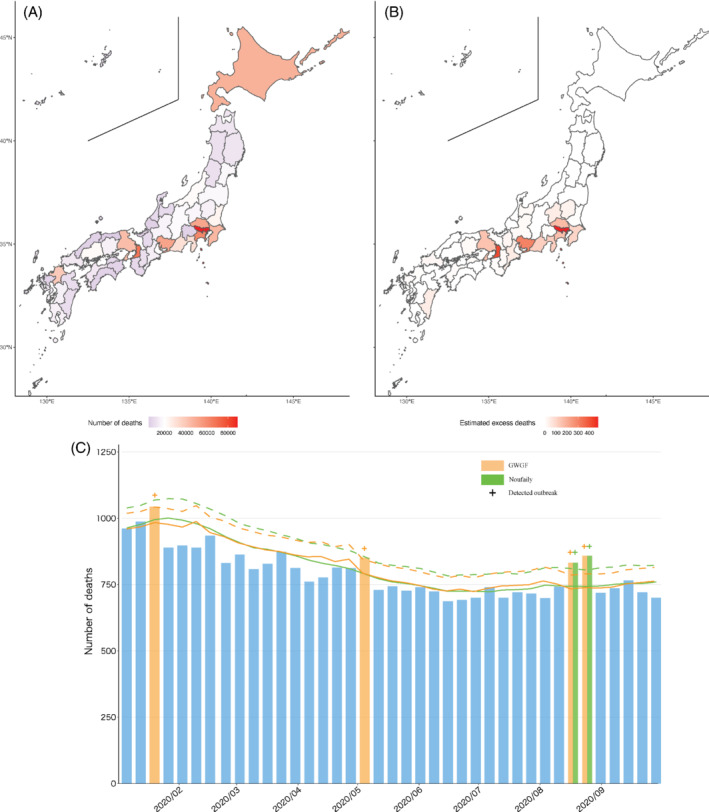
Excess death during January to September 2020, under COVID‐19 pandemic in Japan, A, B, and the time‐series death count and the detected outbreak in the 22th prefecture, C: Green is Noufaily method, red is GWGF method, dagger (“+”) is outbreak week, solid line is expected number of deaths, and dashed line is 95% upper bound of prediction interval [Colour figure can be viewed at wileyonlinelibrary.com]

TABLE 3.

Number of detected outbreaks and estimated number of excess death during January to September, 2020 under the COVID‐19 pandemic in Japan

		Number of estimated deaths		Number of detected outbreaks		Number of excess deaths
Prefecture	Number of deaths	Noufaily	GWGF	Noufaily	GWGF	Noufaily	GWGF
Total	1 006 064	1 033 708	1 039 153	60	54	1727	2202
1	47 363	49 303	49 595	0	0	0	0
2	13 055	13 941	13 979	1	0	1	0
3	12 556	13 381	13 464	0	0	0	0
4	17 886	18 889	19 054	0	0	0	0
5	11 268	11 790	11 793	1	0	8	0
6	11 106	11 677	11 695	1	0	4	0
7	17 848	18 415	18 485	0	0	0	0
8	24 140	25 092	25 336	1	1	3	2
9	15 924	16 400	16 522	3	2	31	31
10	17 059	17 545	17 619	2	2	45	44
11	51 492	52 171	52 592	3	3	105	166
12	45 468	46 603	46 929	2	3	116	104
13	88 932	90 754	91 514	3	3	379	477
14	61 837	63 434	63 764	1	1	120	154
15	21 440	22 745	22 837	0	0	0	0
16	9461	9670	9746	2	1	37	16
17	9321	9578	9602	0	0	0	0
18	6798	7065	7115	0	0	0	0
19	7184	7452	7492	1	1	6	5
20	18 558	19 109	19 179	0	0	0	0
21	16 589	17 364	17 445	1	1	8	12
22	31 036	31 911	32 014	2	4	77	121
23	51 904	52 800	53 098	4	5	154	299
24	15 297	15 548	15 655	3	2	45	48
25	9534	9805	9869	2	1	34	24
26	19 938	20 302	20 386	0	1	0	3
27	67 992	69 196	69 435	3	5	286	418
28	43 200	43 630	43 820	2	5	75	150
29	10 844	11 003	11 041	3	1	25	12
30	9256	9593	9643	1	1	12	8
31	5171	5611	5660	0	0	0	0
32	7061	7132	7149	2	0	2	0
33	15 921	16 496	16 529	1	1	13	14
34	22 297	23 331	23 378	0	0	0	0
35	13 697	14 107	14 160	1	1	18	20
36	7251	7452	7471	1	0	7	0
37	8924	8991	9007	3	2	19	11
38	13 199	13 456	13 483	1	1	5	9
39	7347	7576	7610	0	0	0	0
40	39 363	40 489	40 730	0	1	0	3
41	7337	7388	7442	2	1	12	7
42	12 942	13 022	13 043	0	0	0	0
43	15 545	15 893	16 011	0	0	0	0
44	10 472	10 705	10 779	1	0	6	0
45	10 342	10 131	10 184	6	4	74	44
46	15 663	16 222	16 253	0	0	0	0
47	9246	9540	9546	0	0	0	0

5. DISCUSSION

Along with the increasing attention being paid to the rapid surveillance system for emerging infectious diseases, such as COVID‐19, there is a higher demand for predictive approaches with rapid and higher accuracy of outbreak detection. Notably, when the number of time points in the available dataset is not so high, that is, when the data has not been accumulated for a long time period, the detection accuracy might be limited because of the large standard error in the regression parameter estimates. This study demonstrates a novel method, the GWGF algorithm, to incorporate geographical information with quasi‐Poisson regression to detect outbreaks in timely manner, which can be considered as a natural generalization of Farrington et al ⁶ and Noufaily et al. ⁷ The novel feature of the new method entails that, as with, ²¹ , ²² , ²³ , ²⁴ it makes use of geographical information as the weights in the quasi‐likelihood for improving the estimation. The weights control the spatial dependency between two locations with a bandwidth parameter, which is optimized based on the qAICc in this study. The preferable detection performance is examined in the extensive numerical experiments and real‐data analysis in Japan during the COVID‐19 pandemic. We show that the GWGF algorithm succeeds in improving recall (or sensitivity) without reducing the level of precision, which means that it can detect true outbreaks (ie, true positive) while maintaining a low number of false positives. ³⁷ This improvement is more evident when using a short period of data, especially in terms of precision. However, the specificity for the non‐outbreak detection is relatively low. Therefore, the use of the different algorithms depending on the situation. In other words, if the detection of an outbreak is the aim, the GWGF algorithm should be used from the perspective of recall and precision; otherwise, we would be requested to also check the results of the conventional Farrington algorithm at the same time. In addition, we note that the application results depend on the choice of the distance metrics, the associated kernel, and the prespecified parameter set $(b,w)$. We (partially) show the results of the sensitivity analysis in terms of the choice of $(b,w)$ in the previous studies, ¹⁸ , ³⁶ and we welcome the re‐evaluation of our method in other settings.

In a rapid surveillance system, this novel algorithm can be used as a new tool for detecting outbreaks and further exploitative spatial analysis to identify the regional heterogeneity of excess death. It works especially when only short‐term data are available because it incorporates the neighborhood data to stabilize the estimation. Furthermore, this article provides a general framework of the geographically weighted version of the quasi‐likelihood approach, including the procedures for estimating the dispersion parameter with local weights and for selecting the optimal bandwidth in the spatial kernel. It implies that it is possible to extend it to other quasi‐likelihood‐based models with geographical weights, such as those discussed in References 38 and 39. In addition, we can incorporate the variable selection approach by using qAIC or a sparse penalty, which has been extensively studied by Yoneoka et al ²⁴ and Wheeler. ⁴⁰ , ⁴¹

Regarding the estimation of the regression coefficient for geographically invariant covariates, $\mathit{\zeta }$, we propose the two‐step procedure: estimate ${\mathit{\zeta }}_j$ for each location, and then average them to estimate $\mathit{\zeta }$. Although the procedure yields a consistent estimator of $\mathit{\zeta }$, it may reduce the estimation efficiency. A possible improvement could be the use of a profile quasi‐likelihood approach or a three‐step procedure. The first step should be to use a relatively large bandwidth to induce undersmoothing estimates of the geographically varying coefficients. Then, these undersmoothing estimates should be fixed to determine $\mathit{\zeta }$. The last step should fix the estimated $\mathit{\zeta }$ with a correctly sized bandwidth. Undersmoothing improves the efficiency of the estimation of $\mathit{\zeta }$. The theoretical guarantee, including the inference of $\mathit{\zeta }$ and other regression parameters, is our ongoing study. However, because it is good for the users of our algorithm to be able to choose the estimation methods, we will introduce these methods in the R package “geoFarrington” and to the GitHub repository in the near future.

We should mention that the idea to combine the geographical weights with spatial kernel and quasi‐likelihood‐based regression models is not new in the field of spatial analysis; ²² , ²³ , ³⁹ however, one of their main focus is to improve the (asymptotic) efficiency of the estimates in the regression model by incorporating the geographical information. Conversely, this study aims to examine and improve the detection performance on how the observed number exceeds the upper prediction band of the model in the context of excess death, which highly depends on several settings, such as the threshold value U, and how to construct the prediction band.

CONFLICT OF INTEREST

The authors declare no potential conflict of interest.

Supporting information

Data S1 Estimated excess deaths during January to September, 2020, under COVID‐19 pandemic in Japan in all 47 prefectures

Yoneoka D, Kawashima T, Makiyama K, Tanoue Y, Nomura S, Eguchi A. Geographically weighted generalized Farrington algorithm for rapid outbreak detection over short data accumulation periods. Statistics in Medicine. 2021;40(28):6277–6294. doi: 10.1002/sim.9182

DATA AVAILABILITY STATEMENT

Note that the R code and R package “geoFarrington” for the proposed method are provided in a GitHub repository (https://github.com/kingqwert/R/blob/master/geoFarrington/geo_farrington_withCovs.R) and will be hosted on the CRAN repository (https://www.r‐project.org/) in the near future, thereby facilitating the application of our method by others. Additionally, they are also available on request from the corresponding author (daisuke.yoneoka@slcn.ac.jp).

REFERENCES

- 1. Farrington P, Andrews N. Application to infectious. Ron Brookmeyer, Donna Stroup, Monitoring the Health of Populations: Statistical Principles and Methods for Public Health Surveillance; UK: Oxford University Press; 2003:203. [Google Scholar]
- 2. Unkel S, Farrington CP, Garthwaite PH, Robertson C, Andrews N. Statistical methods for the prospective detection of infectious disease outbreaks: a review. J Royal Stat Soc Ser A (Stat Soc). 2012;175(1):49‐82. [Google Scholar]
- 3. Shmueli G, Burkom H. Statistical challenges facing early outbreak detection in biosurveillance. Technometrics. 2010;52(1):39‐51. [Google Scholar]
- 4. Buckeridge DL, Burkom H, Campbell M, Hogan WR, Moore AW, et al. Algorithms for rapid outbreak detection: a research synthesis. J Biomed Inform. 2005;38(2):99‐113. [DOI] [PubMed] [Google Scholar]
- 5. Sonesson C, Bock D. A review and discussion of prospective statistical surveillance in public health. J Royal Stat Soc Ser A (Stat Soc). 2003;166(1):5‐21. [Google Scholar]
- 6. Farrington C, Andrews NJ, Beale A, Catchpole M. A statistical algorithm for the early detection of outbreaks of infectious disease. 1996;J Royal Stat Soc Ser A (Stat Soc), 159(3):547‐563. [Google Scholar]
- 7. Noufaily A, Enki DG, Farrington P, Garthwaite P, Andrews N, Charlett A. An improved algorithm for outbreak detection in multiple surveillance systems. Stat Med. 2013;32(7):1206‐1222. [DOI] [PubMed] [Google Scholar]
- 8. Michelozzi P, de'Donato F, Scortichini M, et al. Temporal dynamics in total excess mortality and covid‐19 deaths in Italian cities. BMC Public Health. 2020;20(1):1‐8. [DOI] [PMC free article] [PubMed] [Google Scholar]
- 9. Krieger N, Chen JT, Waterman PD. Excess mortality in men and women in Massachusetts during the covid‐19 pandemic. Lancet. 2020;395(10240):1829. [DOI] [PMC free article] [PubMed] [Google Scholar]
- 10. Banerjee A, Pasea L, Harris S, et al. Estimating excess 1‐year mortality associated with the covid‐19 pandemic according to underlying conditions and age: a population‐based cohort study. Lancet. 2020;395(10238):1715‐1725. [DOI] [PMC free article] [PubMed] [Google Scholar]
- 11. Burki T. England and wales see 20 000 excess deaths in care homes. Lancet. 2020;395(10237):1602. [DOI] [PMC free article] [PubMed] [Google Scholar]
- 12. EUROMOMO. EuroMOMO Bulletin, Week 3; 2021.
- 13. Vestergaard LS, Nielsen J, Richter L, et al. Excess all‐cause mortality during the covid‐19 pandemic in Europe–preliminary pooled estimates from the Euromomo network, March to April 2020. Eurosurveillance. 2020;25(26):2001214. [DOI] [PMC free article] [PubMed] [Google Scholar]
- 14. Vestergaard LS, Nielsen J, Krause TG, et al. Excess all‐cause and influenza‐attributable mortality in Europe, December 2016 to February 2017. Eurosurveillance. 2017;22(14):30506. [DOI] [PMC free article] [PubMed] [Google Scholar]
- 15. Centers for Disease Control and Prevention Excess deaths associated with COVID‐19; 3, 2021.
- 16. Wu J, Mafham M, Mamas M, et al. Place and underlying cause of death during the covid‐19 pandemic: retrospective cohort study of 3.5 million deaths in England and wales, 2014 to 2020. Mayo Clin Proc. 2021;96(4):952–963. [DOI] [PMC free article] [PubMed] [Google Scholar]
- 17. Al Wahaibi A, Al‐Maani A, Alyaquobi F, et al. Effects of covid‐19 on mortality: a 5‐year population‐based study in Oman. Int J Infect Dis. 2021;104:102‐107. [DOI] [PMC free article] [PubMed] [Google Scholar]
- 18. Kawashima T, Nomura S, Tanoue Y, et al. Excess all‐cause deaths during coronavirus disease pandemic, Japan, January–May 2020. Emerg Infect Dis. 2021;27(3):789. [DOI] [PMC free article] [PubMed] [Google Scholar]
- 19. Buckeridge DL. Outbreak detection through automated surveillance: a review of the determinants of detection. J Biomed Inform. 2007;40(4):370‐379. [DOI] [PubMed] [Google Scholar]
- 20. Noufaily A, Morbey RA, Colón‐González FJ, et al. Comparison of statistical algorithms for daily syndromic surveillance aberration detection. Bioinformatics. 2019;35(17):3110‐3118. [DOI] [PMC free article] [PubMed] [Google Scholar]
- 21. Fotheringham AS, Brunsdon C, Charlton M. Geographically Weighted Regression: The Analysis of Spatially Varying Relationships. Chichester: John Wiley & Sons; 2003. [Google Scholar]
- 22. Wu J‐W. The quasi‐likelihood estimation in regression. Ann Inst Stat Math. 1996;48(2):283‐294. [Google Scholar]
- 23. Loader C. Local Regression and Likelihood. New York, NY: Springer Science & Business Media; 2006. [Google Scholar]
- 24. Yoneoka D, Saito E, Nakaoka S. New algorithm for constructing area‐based index with geographical heterogeneities and variable selection: an application to gastric cancer screening. Sci Rep. 2016;6(1):1‐7. [DOI] [PMC free article] [PubMed] [Google Scholar]
- 25. Nakaya T, Fotheringham AS, Brunsdon C, Charlton M. Geographically weighted poisson regression for disease association mapping. Stat Med. 2005;24(17):2695‐2717. [DOI] [PubMed] [Google Scholar]
- 26. Zhang W, Lee S‐Y, Song X. Local polynomial fitting in semivarying coefficient model. J Multivar Anal. 2002;82(1):166‐188. [Google Scholar]
- 27. Brunsdon C, Fotheringham S, Charlton M. Geographically weighted regression. J Royal Stat Soc Ser D (Stat). 1998;47(3):431‐443. [Google Scholar]
- 28. Davison A, Snell E. Residuals and diagnostics. Stat Theory Mod. 1991.in honour of Sir David Cox, FRS:83–106. [Google Scholar]
- 29. Bartlett MS. The use of transformations. Biometrics. 1947;3(1):39‐52. [PubMed] [Google Scholar]
- 30. Höhle M. surveillance: an r package for the monitoring of infectious diseases. Comput Stat. 2007;22(4):571‐582. [Google Scholar]
- 31. Hastie T, Tibshirani R. Varying‐coefficient models. J Royal Stat Soc Ser B (Methodol). 1993;55(4):757‐779. [Google Scholar]
- 32. McCullagh P. Quasi‐likelihood functions. Ann Stat. 1983;11:59‐67. [Google Scholar]
- 33. Fan J, Zhang W. Statistical methods with varying coefficient models. Stat Interf. 2008;1(1):179. [DOI] [PMC free article] [PubMed] [Google Scholar]
- 34. Hurvich CM, Tsai C‐L. Bias of the corrected AIC criterion for underfitted regression and time series models. Biometrika. 1991;78(3):499‐509. [Google Scholar]
- 35. Maëlle S, Dirk S, Michael H. Monitoring count time series in R: aberration detection in public health surveillance; 2014. arXiv preprint arXiv:1411.1292.
- 36. National Institute of Infectious Diseases Excess Death in Japan; March 2021.
- 37. Steyerberg EW. Clinical Prediction Models. New York, NY: Springer; 2019. [Google Scholar]
- 38. Carroll RJ, Ruppert D, Welsh AH. Local estimating equations. J Am Stat Assoc. 1998;93(441):214‐227. [Google Scholar]
- 39. Fan J, Heckman NE, Wand MP. Local polynomial kernel regression for generalized linear models and quasi‐likelihood functions. J Am Stat Assoc. 1995;90(429):141‐150. [Google Scholar]
- 40. Wheeler DC. Diagnostic tools and a remedial method for collinearity in geographically weighted regression. Environ Plan A. 2007;39(10):2464‐2481. [Google Scholar]
- 41. Wheeler DC. Simultaneous coefficient penalization and model selection in geographically weighted regression: the geographically weighted lasso. Environ Plan A. 2009;41(3):722‐742. [Google Scholar]
Associated Data
This section collects any data citations, data availability statements, or supplementary materials included in this article.
Supplementary Materials