Study becomes insight: Ecological learning from machine learning

Abstract

1. The ecological and environmental science communities have embraced machine learning (ML) for empirical modelling and prediction. However, going beyond prediction to draw insights into underlying functional relationships between response variables and environmental ‘drivers’ is less straightforward. Deriving ecological insights from fitted ML models requires techniques to extract the ‘learning’ hidden in the ML models.

2. We revisit the theoretical background and effectiveness of four approaches for deriving insights from ML: ranking independent variable importance (Gini importance, GI; permutation importance, PI; split importance, SI; and conditional permutation importance, CPI), and two approaches for inference of bivariate functional relationships (partial dependence plots, PDP; and accumulated local effect plots, ALE). We also explore the use of a surrogate model for visualization and interpretation of complex multi‐variate relationships between response variables and environmental drivers. We examine the challenges and opportunities for extracting ecological insights with these interpretation approaches. Specifically, we aim to improve interpretation of ML models by investigating how effectiveness relates to (a) interpretation algorithm, (b) sample size and (c) the presence of spurious explanatory variables.

3. We base the analysis on simulations with known underlying functional relationships between response and predictor variables, with added white noise and the presence of correlated but non‐influential variables. The results indicate that deriving ecological insight is strongly affected by interpretation algorithm and spurious variables, and moderately impacted by sample size. Removing spurious variables improves interpretation of ML models. Meanwhile, increasing sample size has limited value in the presence of spurious variables, but increasing sample size does improves performance once spurious variables are omitted. Among the four ranking methods, SI is slightly more effective than the other methods in the presence of spurious variables, while GI and SI yield higher accuracy when spurious variables are removed. PDP is more effective in retrieving underlying functional relationships than ALE, but its reliability declines sharply in the presence of spurious variables. Visualization and interpretation of the interactive effects of predictors and the response variable can be enhanced using surrogate models, including three‐dimensional visualizations and use of loess planes to represent independent variable effects and interactions.

4. Machine learning analysts should be aware that including correlated independent variables in ML models with no clear causal relationship to response variables can interfere with ecological inference. When ecological inference is important, ML models should be constructed with independent variables that have clear causal effects on response variables. While interpreting ML models for ecological inference remains challenging, we show that careful choice of interpretation methods, exclusion of spurious variables and adequate sample size can provide more and better opportunities to ‘learn from machine learning’.

1. THE NEED TO IMPROVE MACHINE LEARNING INTERPRETABILITY IN ECOLOGY

Ecologists and environmental scientists often find themselves searching for tools to model and predict complex, nonlinear and high‐dimensional systems. In recent years, our ability to predict complicated systems has greatly improved through the development of machine learning (ML) algorithms. A substantial body of literature has accumulated on applications of ML in the ecological and environmental sciences (e.g. Cutler et al., ²⁰⁰⁷; Elith & Leathwick, ²⁰¹⁷; Elith et al., ²⁰⁰⁸; Marmion et al., ²⁰⁰⁹). However, when prediction is not the primary goal, most ML methods tend to behave like ‘black boxes’, meaning that it can be challenging to derive new understanding or ecological insights from these statistical models, irrespective of their predictive abilities (Roscher et al., 2020). For example, if we are interested in understanding the distribution of species richness sampled across a study domain (the ‘response’ variable), we might use ML methods to fit relationships with a set of candidate independent (‘predictor’) variables (e.g. variables describing the spatial and temporal variation in climate, soils and disturbance). The resulting ML model may closely fit the training data and provide accurate predictions for locations between sample plots. However, without appropriate visualization or interpretation tools, that same model may provide little or no insight into the functional (or causal) relationships between species diversity and underlying climatic, edaphic and biotic interactions.

The ability of ML approaches to predict accurately is valuable, but ecological interpretation of the underlying functional relationships can be challenging (Lucas, 2020; Wenger & Olden, ²⁰¹²). Nonetheless, the often superior predictive ability of ML approaches, relative to more traditional approaches (e.g. linear and nonlinear regression), suggests that the functional relationships are embodied in the fitted ML models. The challenge, therefore, is to provide tools to extract (quantify and/or visualize) those functional and ecological relationships from the black box. In particular, we would hope that ML will help answer three key ecological questions: (a) Which predictor variables are the most influential in determining the behaviour of the response variable? (b) What are the functional relationships between predictors and the response variable? And (c) how do interactions among predictors determine the complex and often nonlinear patterns in the response variable?

To extract ecological insights, we need a comprehensive understanding of interpretation approaches for ML models and how to generate reliable and accurate interpretation results (Brieuc et al., 2018; Cutler et al., ²⁰⁰⁷; Lucas, ²⁰²⁰). Earlier studies focused on the accuracy of variable importance estimations (Gini impurity and mean decrease in accuracy) related to impacts of correlated predictors (e.g. Gregorutti et al., 2017; Strobl et al., ²⁰⁰⁸), scale of measurement and number of categories (e.g. Nicodemus, ²⁰¹¹; Strobl et al., ²⁰⁰⁷) and their intrinsic stability (Calle & Urrea, 2011; Wang et al., ²⁰¹⁶). Mean decrease in accuracy is sensitive to dataset noise (Calle & Urrea, 2011), while the performance of the Gini coefficient is affected by correlation between predictor variables and the number of categories for categorical predictors (Nicodemus, 2011). While agreement has not been reached for which of the two is more efficient (e.g. Calle & Urrea, ²⁰¹¹; Nicodemus, ²⁰¹¹), new variable importance measures have been developed (e.g. conditional importance by Strobl et al., ²⁰⁰⁷ and split importance [SI] by Elith et al., ²⁰⁰⁸), promoting the need for a comprehensive comparison among them. Meanwhile, compared to variable importance, assessment for methods to extract bivariate relationships has received much less attention, although it is critical for ecological interpretation.

The need for sufficient training data (sample size) has long been a major concern for accurate ML model predictions (Perry & Dickson, 2018; Raudys & Jain, ¹⁹⁹¹; Stockwell & Peterson, ²⁰⁰²). However, it is less well‐known how sample size impacts model interpretation, including variable importance and functional relationships. This is particularly important in ecology, where relatively small‐scale experiments lead to ML models with small sample sizes. Assessment of variable importance measures (Gini and permutation importance) showed that both of them are sensitive to sample size (e.g. Strobl & Zeileis, 2008; Wang et al., ²⁰¹⁶). Similarly, while the presence of spurious variables may have little negative impact on ML predictions, the covariance among true and spurious predictors may reduce our ability to effectively rank predictor importance. More particularly, the inclusion of spurious predictor variables will likely obscure our ability to retrieve ‘true’ functional relationships for influential predictors, as spurious variables alias a portion of the underlying correlations with true predictors and thus obscure the true relationships.

In this paper, we evaluate how ML interpretation approaches are impacted by sample size and the presence of spurious variables. We review interpretive tools that can shed new light on the ML black box, and provide opportunities for new and improved ecological and functional insights. We use a simulation dataset to illustrate key interpretation strategies, and demonstrate their abilities for reliable ecological interpretation and inference. In so doing, we provide some recommendations for efficient ecological interpretation.

2. MATERIALS AND METHODS

We conducted a simulation, with known underlying relationships between response and predictor variables, to assess retrieval of ecological insights from ML models. We examine four algorithms to evaluate variable importance and two for visualization of bivariate functional relationships between each predictor and the response variable. We then introduce surrogate models to visualize the interactive (i.e. multivariate) effects of predictor variables on the response variable. We provide brief theoretical background for the interpretation approaches, compare their performance and analyse their sensitivity to sample size and spurious variables.

2.1. Simulation design

We generated a pseudo dataset representing hypothetical variability in global species richness in response to three environmental predictors, with known underlying functional relationships (Figure 1a). To fulfil the goal of examining effectiveness of ML interpretation approaches, our simulation simplified and generalized the abiotic mechanisms of species richness by focusing on three primary factors: temperature (MAT, K; Antão et al., ²⁰²⁰; Fuhrman et al., ²⁰⁰⁸; Stegen et al., ²⁰¹²), rainfall (MAP, mm; Frank et al., ²⁰¹⁴; Gelfand et al., ²⁰⁰⁵) and disturbance (here we only used fire frequency, year⁻¹; He et al., ²⁰¹⁹; Peterson & Reich, ²⁰⁰⁸). In this hypothetical example, we modelled species richness (SN) as a linear combination of the three environmental (predictor) variables:

$${\text{SNnorm}}_x=f\left(x\right)+\epsilon ,$$ (1)

$$\text{SN}=100\times \left(w_1\times {\text{SNnorm}}_{\text{MAT}}+w_2\times {\text{SNnorm}}_{\text{MAP}}+w_3\times {\text{SNnorm}}_{\text{Fire}}\right),$$ (2)

where x represents each of the three predictors (MAT, MAP and fire), and $\mathrm{f}$ is the associated deterministic function. SNnorm _x (each scaled 0–1) are the normalized species richness values determined by environmental predictors x. The three SNnorm _x (Figure 1a) were generated with parabolic, sigmoid and negative sigmoid relationships (f) for MAT, MAP and fire frequency, respectively, with added Gaussian error (ε). Weights (w) for MAT, MAP and fire frequency were set as w ₁ = 0.6, w ₂ = 0.3 and w ₃ = 0.1, respectively, representing the relative importance of the three predictors in determining eventual SN. We constrained the range of SN to 0–100 by removing points (166 samples) out of the 0–100 range.

FIGURE 1.

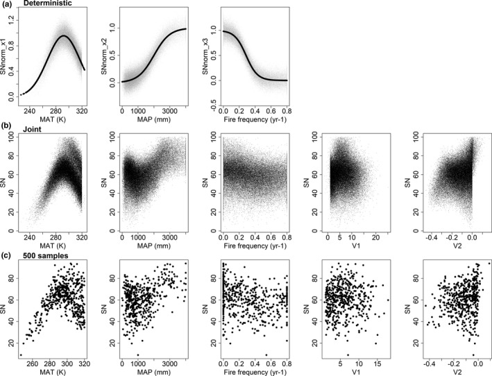
Simulated relationships between species richness for a hypothetical taxon and five environmental predictor variables. The upper row (a) shows the deterministic bivariate relationships (dark line) used to simulate species richness (Equation 1), with additional Gaussian noise (grey points). Row (b) shows the final species richness (SN, Equation 2) along the five predictors under ‘data‐rich’ scenario (N = 64,454). Row (c) illustrates the additional challenge inherent in modelling data‐poor situations, showing 500 samples randomly selected from row (b)

In addition, we simulated two environmental variables, ‘V1’ and ‘V2’, which in our simulation have varying degree of correlation with the three (‘true’) predictor variables, but no direct impact on species richness. These ‘spurious variables’ were included in the ML analysis to mimic common practice of including numerous variables when constructing ML models, many of which are mechanistically uninfluential in determining the response, but may nevertheless be correlated with it due to environmental covariance. The combination of correlation among predictor variables and noise obscures the underlying bivariate relationships (Figure 1).

Simulation of the five environmental variables incorporated hypothetical spatial gradients in a domain representing a hypothetical terrestrial world, with partial covariance among environmental variables, as typically found in real systems (Figure 2). Thus among the three ‘true’ predictor variables, MAT follows a latitudinal gradient peaking near the equator (Figure 2a); MAP peaks in the centre of the domain and declines outwards (Figure 2b); while fire frequency interacts with MAP and MAT, peaking in mesic systems with moderate rainfall and higher temperature (Figure 2c). Among the two ‘spurious variables’, V1 (Figure 2d) increases from west to east with no direct dependence on other predictors, while V2 (Figure 2e) is partially correlated with the other predictor variables.

FIGURE 2.

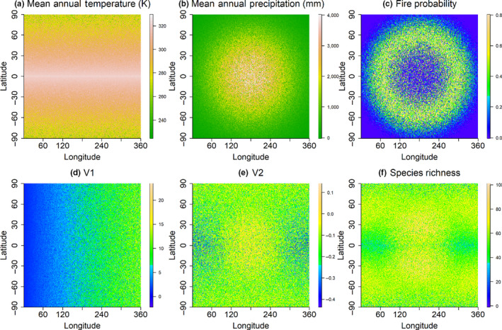
Spatial distribution of three influential environmental variables: (a) temperature, (b) precipitation and (c) fire, and two non‐influential variables: (d) V1 and (e) V2 used to model (f) species richness generated using Equation 1

Weight terms (w) in Equation 2 provide the underlying variable importance, ranked MAT > MAP > fire frequency. The deterministic relationships in Figure 1a represent the underlying functional relationships between species richness and the three deterministic predictors, while the spatial interactions among predictors (Figure 2) simulate covariance among predictors that tends to confound the ability of statistical modelling approaches to derive accurate functional relationships, particularly when examined using bivariate methods (Figure 1b,c). As is common in real‐world situations, the spatial interactions between predictor variables distort our ability to visualize bivariate relationships (Figure 1b,c), particularly for variables with lower influence such as mean annual precipitation and fire frequency (w = 0.3 and 0.1 respectively). Our goal, therefore, is to be able to work with complex, correlated and noisy data, such as simulated here, and discern which predictor variables are ecologically important, and then gain insights into the functional relationships with the response variable.

2.2. Interpretation methods

We investigated interpretation approaches for extracting (a) variable importance, (b) bivariate functional relationships and (c) multi‐variate functional relationships and predictor interactions. For each interpretation approach, we examined how they are affected by sample size and spurious variables.

We used random forest (RF) and boosted regression tree (BRT) models as our primary ML examples, although many of the insights and recommendations apply to other common ML approaches. RF and BRT are used extensively in ecology and environmental sciences, in large part due to their ability to deal with nonlinear interactions and remarkable predictive capabilities (e.g. Anchang et al., ²⁰²⁰; Brieuc et al., ²⁰¹⁸; Cutler et al., ²⁰⁰⁷; De'Ath, ²⁰⁰⁷; Jevšenak & Skudnik, ²⁰²¹; Molnar, ²⁰¹⁹; Prasad et al., ²⁰⁰⁶; Ross et al., ^{2020; 2021}). The hyperparameters used for ML models were consistent among sample size and bootstraps. We used 100 trees for RF, while the number of predictors (mtry) was determined using the tuneFR function. For BRT, the tree complexity was three, learning rate equalled 0.01 and bag fraction was 0.8. The predicted species richness by RF and BRT and associated predictor errors are shown in Figure S1. The pseudo dataset comprised 64,620 (359 × 180) samples, representing species richness across the hypothetical domain (Figure 2f). Since real‐world studies can be severely data limited, we also sampled the full dataset (sample sizes: 100, and from 500 to 5,500 with an interval of 500) to examine how dataset size affects ML interpretation. To avoid spurious findings with random sample fluctuations, the random selection of samples was bootstrapped with 100 repetitions (the distribution of bootstrap samples with respect to predictor variables was checked for similarity with the overall dataset using Kolmogorov–Smirnov test).

2.2.1. Variable importance

Variable importance (or feature importance) approaches are designed to rank the relative contribution of multiple predictor variables to response variables in ML models (Friedman, 2001). There is little consensus in the ML literature on how to calculate the relative importance of different independent variables in a fitted model. We tested four frequently used methods to rank predictor variables: Gini importance (GI; Breiman, ²⁰⁰¹), permutation importance (PI; Cutler et al., ²⁰¹²), conditional permutation importance (CPI; Strobl et al., ²⁰⁰⁷) and (SI; Elith et al., ²⁰⁰⁸). We estimated their accuracy in ranking predictor variables relative to simulated weights (w), and examined their sensitivity to sample size and spurious variables.

The first three importance measurements are associated with RF model, while the last one (SI) is commonly used with BRT models. GI quantifies the decreased variation of samples through all the nodes split by a predictor variable in a RF. PI estimates variable importance as the decrease in prediction accuracy (increase in error) when the target variable is randomized (permuted) and input to a previously trained model (Strobl et al., ,2007, 2008). GI and PI are implemented in the R package randomforest. R package party modifies the PI approach as the CPI, which computes the decrease in prediction accuracy following the permutation of portions of the range of a predictor variable (Strobl et al., 2008). SI considers how many times a predictor variable is used in splits across all trees in a boosted regression tree, and has been adopted by many packages such as lightgbm (Ke et al., 2017), xgboost (Chen & Guestrin, 2016) and brt (Elith et al., 2008; Friedman & Meulman, ²⁰⁰³). See Table S1 for common R resources for ML.

2.2.2. Bivariate functional relationships

We explored two methods, partial dependence plots (PDPs) and accumulated local effects (ALEs), for retrieval of underlying bivariate functional relationships. PDP has been a mainstay for ecological and environmental inference (e.g. Cutler et al., ²⁰⁰⁷; Friedman & Meulman, ²⁰⁰³; Galkin et al., ²⁰¹⁸; Moya‐Laraño & Corcobado, ²⁰⁰⁸; Sankaran et al., ²⁰⁰⁸), while the use of ALE method has been less frequently adopted (Apley & Zhu, 2016). These two approaches are available in most ML programming packages (Table S1). Both PDP and ALE are designed to retrieve the functional relationships between response variables and predictive variables, somewhat analogous to a bivariate linear or nonlinear regression. PDP estimates the marginal effects of predictors by averaging the predicted outcomes from an ML model (Casalicchio et al., 2018; Friedman, ²⁰⁰¹; Molnar et al., ²⁰¹⁸; Zhao & Hastie, ²⁰²¹). By contrast, ALE calculates the difference of local predictions across small intervals of the predictor variable range (Apley & Zhu, 2016). PDP and ALE can be applied to both RF and BRT.

2.2.3. Multi‐variate functional relationships and predictor interactions

While PDP and ALE are intended to show the bivariate relationship between the response variable and predictor variables, the multivariate effects of predictor variables are not readily apparent using bivariate visualizations. A less common approach for visualization of these underlying relationships in the environmental and ecological literature uses interpretable or ‘surrogate’ models (Molnar, 2019). A surrogate model uses predictions from an ML model that are re‐analysed using a more easily interpretable (visualizable) model approach. Although any interpretable model (e.g. a simple decision tree, generalized linear or additive models) can be used as a surrogate model (Molnar et al., 2018), here we highlight the use of three‐dimensional (3D) plane fitting (loess models) as a straightforward approach to visualization of multi‐variate functional relationships and predictor interactions (Aho, 2013).

The surrogate model was generated from the fitted ML model (e.g. using the predict function in R) for all points in the calibration set, potentially enhanced with additional random points in data‐poor situations. In this way, a surrogate model can represent the relationships embodied in the ML model, free of the noise associated with the original data. To explore surrogate model visualizations for ecological interpretation of fitted ML models, we examined the multivariate effect of the more influential variables on species richness using 3D loess planes to show the interactive effect of predictor pairs on the response variable.

3. RESULTS

3.1. Variable importance

We compared the estimated variable importance and the rank of the predictor variables with the simulated importance weights (Figures 3 and 4). In the presence of spurious variables (Figure 3), GI, SI and CPI were able to retrieve the correct rank order among influential variables (MAT > MAP > Fire), and SI showed slightly better result than the others. However, GI and SI assigned considerable importance to the spurious variables (V1, V2) and no method was able to consistently retrieve the applied weightings for the true predictors (w = 60%, 30% and 10% respectively) when spurious variables (V1, V2) were present in the models. PI was unable to correctly rank predictor variables (Figure 3), indicating particular sensitivity of this index to covariance and aliasing among true and spurious variables. Notably, CPI tends to exaggerate the importance of the more important variable (MAT), while assigning relatively low importance to less influential (but true) variables (MAP, fire) and spurious variables. CPI importance rankings were also much more variable than other importance methods. Larger sample size decreases the variation in importance estimates, but did not consistently improve accuracy indicating that, in the presence of spurious predictors, larger sample sizes will not necessarily improve predictor importance assessments.

FIGURE 3.

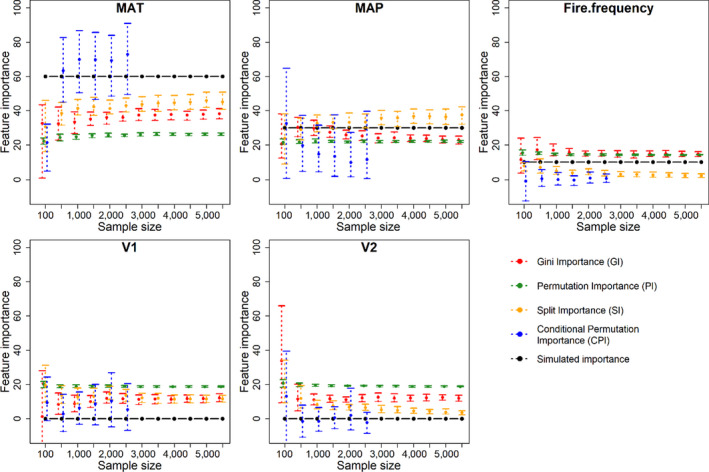
Estimation of feature importance (%) using four interpretation methods as a function of sample size (100, then from 500 to 5,500 with an interval of 500). Points represent mean value of 100 bootstraps, and error bars indicate variation

FIGURE 4.

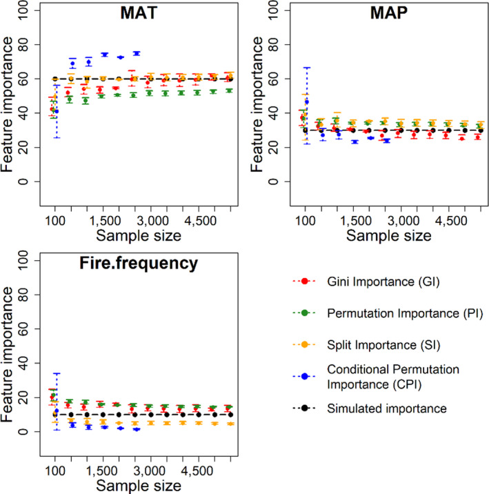
Estimated feature importance (%) for the three ‘true’ predictor variables using four interpretation methods with the two spurious variables omitted in the machine learning models

Removal of spurious variables considerably improved the ability of GI, PI and SI to accurately rank and quantify predictor importance (Figure 4). However, CPI still tends to exaggerate importance of the more influential variable (MAT) while underestimating the less influential variables (MAP and fire). Larger sample sizes, in the absence of spurious variables, improved the ability of GI and PI to retrieve the importance of the three predictors. However, SI and CPI were insensitive to larger sample sizes. In the absence of spurious variables, GI and SI were the most reliable importance indices.

3.2. Bivariate functional relationships

The accuracy assessment for retrieved bivariate functional relationships was conducted using a similarity measure (Kendall's Tau; Sen, 1968) between the retrieved curve and the simulated function for deterministic predictors. A high similarity value indicates that the retrieved functional relationship is similar to the deterministic function (Figure 1a).

Partial dependence plots were generally more accurate than ALE in retrieving the functional form of deterministic variables (Figure 1a), when computed using either the RF or BRT model (Figures S2 and S3). With the existence of spurious variables, increasing sample size has limited effect on the accuracy of either PDP or ALE to retrieve bivariate functions of the three deterministic variables (Figures 5 and 6). Retrieval of functional forms for the three deterministic variables is greatly improved following removal of spurious variables from the models (Figure 6). Figure S3 shows an example of largely improved retrieved curves for the three deterministic variables (either by PDP or ALE) with the spurious variables omitted. The similarity between the retrieved function (by PDP) and the simulated function increased from 0.5 to 0.8 for MAT, from 0.7 to 0.9 for MAP and from 0 to 0.8 for fire frequency, indicating the strong impact of spurious variables on retrieval of bivariate functions. Increasing sample size also tends to improve the accuracy of PDP and ALE, when the spurious variables are excluded, up to a threshold of ~2,000 points beyond which accuracy reaches an asymptote in these simulations.

FIGURE 5.

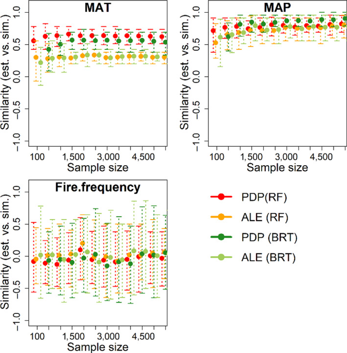
Similarity (Kendall's Tau between retrieved functional curve and the simulated function for the deterministic variables: MAT, MAP and fire frequency) assessment as a function of sample size. At each sample size, the distribution of similarity was generated by the 100 bootstraps. Points represent mean value of similarity among the 100 bootstraps, and error bars indicate variation

FIGURE 6.

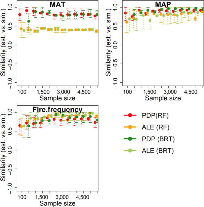
Error/similarity assessment of retrieved functional relationships compared to simulated functional relationships for the three ‘true’ predictor variables, with spurious variables removed

3.3. Multi‐variate functional relationships and predictor interactions

We used 3D loess planes to show how the response variable in our simulations varies with interacting pairs of the three influential variables (MAT, MAP and fire frequency). The simulated data are shown as points and the predictions from the fitted RF model (i.e. the surrogate model) are the planes. As might often occur in real‐world data, the full representation of a predictor variable's functional range does not always occur, leading to concentration of data in parts of the feature space, and less well‐supported loess predictions in under‐sampled regions of feature space. However, the separate and interactive effects of the predictor variables begin to emerge in the shape of the surrogate models. For example, in Figure 7a, which shows simulated species richness response to the two most influential variables (MAT and MAP), the underlying effects of MAT are seen as a bell‐shape distribution, with the asymptotic relationship between species richness and MAP. In our simulated dataset, the fire effect leads to a reduction in species richness but the relationship is complex reflecting realistic correlations between fire frequency and climate that were incorporated into the pseudo‐data simulations (Kahiu & Hanan, 2018).

FIGURE 7.

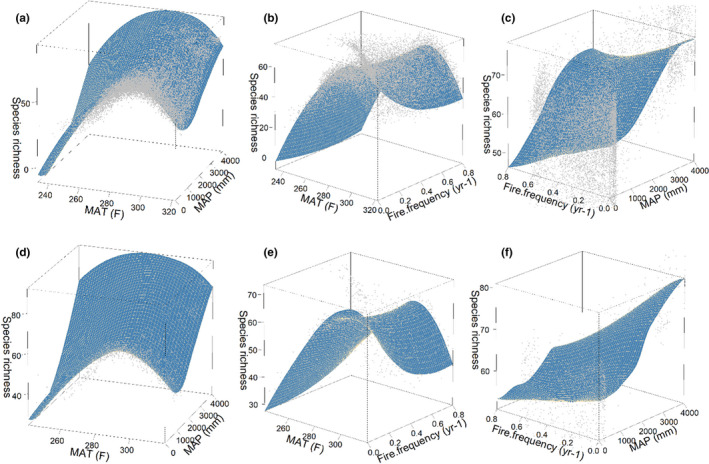
3D loess planes showing how a response variable (species richness) varies with the three deterministic predictor variables (MAT, MAP and fire frequency) with prediction from random forest for a data‐rich scenario (a–c with 5,500 samples) and a data‐poor scenario (d–f with 1,000 samples). Shaded blue planes are the surrogate models. Points are the original stochastically simulated data with known underlying functional relationships (Figure 1a)

The surrogate model predictions for data‐poor models (Figure 7d–f) are broadly similar to data‐rich models but with less reliable predictions of separate and interactive effects, particularly in the already data‐limited extremes of feature space. With limited data samples (1,000 in this case), the interactive effects emerging for the three influential variables are less clear. For example, the effect of fire frequency on species richness at low MAT shifted from the original nearly no effect (Figure 7b) to a conspicuous linear increasing curve (Figure 7e). Meanwhile, fire frequency, simulated with limited effect on specie richness under heavy rainfall due to high moisture (Figure 7c), presented significant negative impact on species richness with small sample size (Figure 7f).

4. DISCUSSION: TOWARDS EFFICIENT ML MODEL INTERPRETATION

Machine learning models have been used extensively in ecological and environmental studies due to their simplicity in implementation and remarkable predictive ability. However, the ‘black box’ nature of most ML models limits ecological inference, process understanding and interpretation of the dynamics underlying the system being studied. In this paper, we reviewed several ML interpretation methods (four variable importance measurements, two functional relationship methods and a surrogate model) and examined their response to sample size and spurious variables, in an effort to improve ecological/process inferences, and make recommendations for use of ML models. We found that the performance of interpretation approaches used to identify which variables are most influential, and retrieve underlying functional relationships from ML models, is sensitive to methods selected and the presence of spurious variables. Increasing sample size improves interpretation when spurious variables are omitted from ML model fits. However, increasing sample size does not, on its own, overcome model confusion caused by spurious variables.

The inclusion of spurious variables (i.e. variables that are correlated with, but do not have a causal relationship with the target variable) severely impacts variable importance ranking and retrieval of functional curves. In particular, removing spurious variables can largely improve variable ranking using GI and SI, likely due to their sensitivity to within‐predictor correlation (Nicodemus, 2011). In our simulations, the PDP approach was considerably more successful than ALE in retrieving underlying functional relationship. However, both methods were highly sensitive to the presence of spurious variables. As found for variable importance ranking, increasing sample size provided little benefit in the ability of PDP and ALE when the spurious variables were present, but increasing sample size did result in improved functional relationship retrieval when spurious variables were excluded.

Our results confirm previous research that careful selection of independent variables is essential for successful ML (e.g. Alizadeh et al., ²⁰¹⁸; Seyedzadeh et al., ²⁰¹⁹; Vellido et al., ²⁰¹²). Although inclusion of numerous independent variables in ML models can yield improvements in predictive ability, this approach is not helpful when ecological interpretation is the goal. We also showed that the use of surrogate models (i.e. analysis of predictions from fitted ML models) can provide additional insights into multi‐variate relationships and predictor interactions using, in this study, 3D loess planes. However, the surrogate model predictions were also very sensitive to dataset size, requiring larger datasets (>1,000 in this case) to characterize the interactive effects of predictor variables.

This study compared different interpretation methods for estimating variable importance and functional relationships and analysed the factors that may influence the interpretation of ML models. ML analysts should be aware that including correlated independent variables in ML models with no clear causal relationship to response variables can interfere with ecological inference. When ecological inference is important, ML models should be constructed with independent variables that have clear causal effects on response variables. While interpretation of ML models for ecological inference remains challenging, careful choice of interpretation methods, exclusion of spurious variables and sufficient sample size can provide ML users with more and better opportunities to ‘learn from machine learning’.

CONFLICT OF INTEREST

The authors declare no conflict of interest.

AUTHORS' CONTRIBUTIONS

N.P.H. and Q.Y. conceived the ideas and designed the simulation model; Q.Y. did the analysis; Q.Y. and W.J. led the writing of the manuscript. All authors contributed critically to writing and editing the drafts and gave the final approval for publication.

PEER REVIEW

The peer review history for this article is available at https://publons.com/publon/10.1111/2041‐210X.13686.

Supporting information

Supplementary Material

Yu, Q. , Ji, W. , Prihodko, L. , Ross, C. W. , Anchang, J. Y. , & Hanan, N. P. (2021). Study becomes insight: Ecological learning from machine learning. Methods in Ecology and Evolution, 12, 2117–2128. 10.1111/2041-210X.13686

DATA AVAILABILITY STATEMENT

The simulation and analysis scripts in R are made available for public at Zenodo https://zenodo.org/badge/latestdoi/387275079 (Yu et al., 2021).

REFERENCES

- Aho, K. A. (2013). Foundational and applied statistics for biologists using R. CRC Press. [Google Scholar]
- Alizadeh, M. J. , Kavianpour, M. R. , Danesh, M. , Adolf, J. , Shamshirband, S. , & Chau, K. W. (2018). Effect of river flow on the quality of estuarine and coastal waters using machine learning models. Engineering Applications of Computational Fluid Mechanics, 12(1), 810–823. 10.1080/19942060.2018.1528480 [DOI] [Google Scholar]
- Anchang, J. Y. , Prihodko, L. , Ji, W. , Kumar, S. S. , Ross, C. W. , Yu, Q. , Lind, B. , Sarr, M. A. , Diouf, A. A. , & Hanan, N. P. (2020). Toward operational mapping of woody canopy cover in tropical savannas using Google Earth Engine. Frontiers in Environmental Science, 8, 4. 10.3389/fenvs.2020.00004 [DOI] [Google Scholar]
- Antão, L. H. , Bates, A. E. , Blowes, S. A. , Waldock, C. , Supp, S. R. , Magurran, A. E. , Dornelas, M. , & Schipper, A. M. (2020). Temperature‐related biodiversity change across temperate marine and terrestrial systems. Nature Ecology & Evolution, 4(7), 927–933. 10.1038/s41559-020-1185-7 [DOI] [PubMed] [Google Scholar]
- Apley, D. W. , & Zhu, J. (2016). Visualizing the effects of predictor variables in black box supervised learning models. ArXiv. 1612.08468. [Google Scholar]
- Breiman, L. (2001). Random forests. Machine Learning, 45(1), 5–32. [Google Scholar]
- Brieuc, M. S. , Waters, C. D. , Drinan, D. P. , & Naish, K. A. (2018). A practical introduction to Random Forest for genetic association studies in ecology and evolution. Molecular Ecology Resources, 18(4), 755–766. 10.1111/1755-0998.12773 [DOI] [PubMed] [Google Scholar]
- Calle, M. L. , & Urrea, V. (2011). Letter to the editor: Stability of random forest importance measures. Briefings in Bioinformatics, 12(1), 86–89. 10.1093/bib/bbq011 [DOI] [PubMed] [Google Scholar]
- Casalicchio, G. , Molnar, C. , & Bischl, B. (2018). Visualizing the feature importance for black box models. In Berlingerio M., Bonchi F., Gärtner T., Hurley N., & Ifrim G. (Eds.), Joint European conference on machine learning and knowledge discovery in databases (pp. 655–670). Springer. [Google Scholar]
- Chen, T. , & Guestrin, C. (2016, August). Xgboost: A scalable tree boosting system. In Proceedings of the 22nd acm sigkdd international conference on knowledge discovery and data mining (pp. 785–794). ACM. [Google Scholar]
- Cutler, A. , Cutler, D. R. , & Stevens, J. R. (2012). Random forests. In Zhang C. & Ma Y. (Eds.), Ensemble machine learning (pp. 157–175). Springer. 10.1007/978-1-4419-9326-7_5 [DOI] [Google Scholar]
- Cutler, D. R. , Edwards, T. C. , Beard, K. H. , Cutler, A. , Hess, K. T. , Gibson, J. , & Lawler, J. J. (2007). Random forests for classification in ecology. Ecology, 88(11), 2783–2792. 10.1890/07-0539.1 [DOI] [PubMed] [Google Scholar]
- De'Ath, G. (2007). Boosted trees for ecological modeling and prediction. Ecology, 88(1), 243–251. https://doi.org/10.1890/0012‐9658(2007)88[243:btfema]2.0.co;2 [DOI] [PubMed] [Google Scholar]
- Elith, J. , & Leathwick, J. (2017). Boosted Regression Trees for ecological modeling. R documentation. Retrieved from https://cran.r‐project.org/web/packages/dismo/vignettes/brt.pdf [Google Scholar]
- Elith, J. , Leathwick, J. R. , & Hastie, T. (2008). A working guide to boosted regression trees. Journal of Animal Ecology, 77(4), 802–813. 10.1111/j.1365-2656.2008.01390.x [DOI] [PubMed] [Google Scholar]
- Frank, A. S. , Wardle, G. M. , Dickman, C. R. , & Greenville, A. C. (2014). Habitat‐and rainfall‐dependent biodiversity responses to cattle removal in an arid woodland–grassland environment. Ecological Applications, 24(8), 2013–2028. 10.1890/13-2244.1 [DOI] [PubMed] [Google Scholar]
- Friedman, J. H. (2001). Greedy function approximation: A gradient boosting machine. The Annals of Statistics, 29(5). 10.1214/aos/1013203451 [DOI] [Google Scholar]
- Friedman, J. H. , & Meulman, J. J. (2003). Multiple additive regression trees with application in epidemiology. Statistics in Medicine, 22(9), 1365–1381. 10.1002/sim.1501 [DOI] [PubMed] [Google Scholar]
- Fuhrman, J. A. , Steele, J. A. , Hewson, I. , Schwalbach, M. S. , Brown, M. V. , Green, J. L. , & Brown, J. H. (2008). A latitudinal diversity gradient in planktonic marine bacteria. Proceedings of the National Academy of Sciences of the United States of America, 105(22), 7774–7778. 10.1073/pnas.0803070105 [DOI] [PMC free article] [PubMed] [Google Scholar]
- Galkin, F. , Aliper, A. , Putin, E. , Kuznetsov, I. , Gladyshev, V. N. , & Zhavoronkov, A. (2018). Human microbiome aging clocks based on deep learning and tandem of permutation feature importance and accumulated local effects. bioRxiv, 507780. [Google Scholar]
- Gelfand, A. E. , Schmidt, A. M. , Wu, S. , Silander, J. A. , Latimer, A. , & Rebelo, A. G. (2005). Modelling species diversity through species level hierarchical modelling. Journal of the Royal Statistical Society: Series C (Applied Statistics), 54(1), 1–20. 10.1111/j.1467-9876.2005.00466.x [DOI] [Google Scholar]
- Gregorutti, B. , Michel, B. , & Saint‐Pierre, P. (2017). Correlation and variable importance in random forests. Statistics and Computing, 27(3), 659–678. 10.1007/s11222-016-9646-1 [DOI] [Google Scholar]
- He, T. , Lamont, B. B. , & Pausas, J. G. (2019). Fire as a key driver of Earth's biodiversity. Biological Reviews, 94(6), 1983–2010. 10.1111/brv.12544 [DOI] [PubMed] [Google Scholar]
- Jevšenak, J. , & Skudnik, M. (2021). A random forest model for basal area increment predictions from national forest inventory data. Forest Ecology and Management, 479, 118601. 10.1016/j.foreco.2020.118601 [DOI] [Google Scholar]
- Kahiu, M. N. , & Hanan, N. P. (2018). Fire in sub‐Saharan Africa: The fuel, cure and connectivity hypothesis. Global Ecology and Biogeography, 27(8), 946–957. 10.1111/geb.12753 [DOI] [Google Scholar]
- Ke, G. , Meng, Q. , Finley, T. , Wang, T. , Chen, W. , Ma, W. , Ye, Q. , & Liu, T. Y. (2017). Lightgbm: A highly efficient gradient boosting decision tree. Advances in Neural Information Processing Systems, 30, 3146–3154. [Google Scholar]
- Lucas, T. C. (2020). A translucent box: Interpretable machine learning in ecology. Ecological Monographs, 90(4), e01422. 10.1002/ecm.1422 [DOI] [Google Scholar]
- Marmion, M. , Parviainen, M. , Luoto, M. , Heikkinen, R. K. , & Thuiller, W. (2009). Evaluation of consensus methods in predictive species distribution modelling. Diversity and Distributions, 15(1), 59–69. 10.1111/j.1472-4642.2008.00491.x [DOI] [Google Scholar]
- Molnar, C. (2019). Interpretable machine learning. A Guide for Making Black Box Models Explainable. https://christophm.github.io/interpretable‐ml‐book/
- Molnar, C. , Casalicchio, G. , & Bischl, B. (2018). Iml: An r package for interpretable machine learning. The Journal of Open Source Software, 3(786), 10–21105. 10.21105/joss.00786 [DOI] [Google Scholar]
- Moya‐Laraño, J. , & Corcobado, G. (2008). Plotting partial correlation and regression in ecological studies. Web Ecology, 8(1), 35–46. 10.5194/we-8-35-2008 [DOI] [Google Scholar]
- Nicodemus, K. K. (2011). Letter to the editor: On the stability and ranking of predictors from random forest variable importance measures. Briefings in Bioinformatics, 12(4), 369–373. 10.1093/bib/bbr016 [DOI] [PMC free article] [PubMed] [Google Scholar]
- Perry, G. L. , & Dickson, M. E. (2018). Using machine learning to predict geomorphic disturbance: The effects of sample size, sample prevalence, and sampling strategy. Journal of Geophysical Research: Earth Surface, 123(11), 2954–2970. [Google Scholar]
- Peterson, D. W. , & Reich, P. B. (2008). Fire frequency and tree canopy structure influence plant species diversity in a forest‐grassland ecotone. Plant Ecology, 194(1), 5–16. 10.1007/s11258-007-9270-4 [DOI] [Google Scholar]
- Prasad, A. M. , Iverson, L. R. , & Liaw, A. (2006). Newer classification and regression tree techniques: Bagging and random forests for ecological prediction. Ecosystems, 9(2), 181–199. 10.1007/s10021-005-0054-1 [DOI] [Google Scholar]
- Raudys, S. J. , & Jain, A. K. (1991). Small sample size effects in statistical pattern recognition: Recommendations for practitioners. IEEE Transactions on Pattern Analysis and Machine Intelligence, 13(3), 252–264. 10.1109/34.75512 [DOI] [Google Scholar]
- Roscher, R. , Bohn, B. , Duarte, M. F. , & Garcke, J. (2020). Explainable machine learning for scientific insights and discoveries. IEEE Access, 8, 42200–42216. 10.1109/ACCESS.2020.2976199 [DOI] [Google Scholar]
- Ross, C. W. , Grunwald, S. , Vogel, J. G. , Markewitz, D. , Jokela, E. J. , Martin, T. A. , Bracho, R. , Bacon, A. R. , Brungard, C. W. , & Xiong, X. (2020). Accounting for two‐billion tons of stabilized soil carbon. Science of the Total Environment, 703, 134615. 10.1016/j.scitotenv.2019.134615 [DOI] [PubMed] [Google Scholar]
- Ross, C. W. , Hanan, N. P. , Prihodko, L. , Anchang, J. , Ji, W. , & Yu, Q. (2021). Woody‐biomass projections and drivers of change in sub‐Saharan Africa. Nature Climate Change, 11(5), 449–455. 10.1038/s41558-021-01034-5 [DOI] [PMC free article] [PubMed] [Google Scholar]
- Sankaran, M. , Ratnam, J. , & Hanan, N. (2008). Woody cover in African savannas: The role of resources, fire and herbivory. Global Ecology and Biogeography, 17(2), 236–245. 10.1111/j.1466-8238.2007.00360.x [DOI] [Google Scholar]
- Sen, P. K. (1968). Estimates of the regression coefficient based on Kendall's tau. Journal of the American Statistical Association, 63(324), 1379–1389. 10.1080/01621459.1968.10480934 [DOI] [Google Scholar]
- Seyedzadeh, S. , Rahimian, F. P. , Rastogi, P. , & Glesk, I. (2019). Tuning machine learning models for prediction of building energy loads. Sustainable Cities and Society, 47, 101484. 10.1016/j.scs.2019.101484 [DOI] [Google Scholar]
- Stegen, J. C. , Ferriere, R. , & Enquist, B. J. (2012). Evolving ecological networks and the emergence of biodiversity patterns across temperature gradients. Proceedings of the Royal Society B: Biological Sciences, 279(1731), 1051–1060. 10.1098/rspb.2011.1733 [DOI] [PMC free article] [PubMed] [Google Scholar]
- Stockwell, D. R. , & Peterson, A. T. (2002). Effects of sample size on accuracy of species distribution models. Ecological Modelling, 148(1), 1–13. 10.1016/S0304-3800(01)00388-X [DOI] [Google Scholar]
- Strobl, C. , Boulesteix, A.‐L. , Kneib, T. , Augustin, T. , & Zeileis, A. (2008). Conditional variable importance for random forests. BMC Bioinformatics, 9(1), 307. 10.1186/1471-2105-9-307 [DOI] [PMC free article] [PubMed] [Google Scholar]
- Strobl, C. , Boulesteix, A. L. , Zeileis, A. , & Hothorn, T. (2007). Bias in random forest variable importance measures: Illustrations, sources and a solution. BMC Bioinformatics, 8(1), 1–21. 10.1186/1471-2105-8-25 [DOI] [PMC free article] [PubMed] [Google Scholar]
- Strobl, C. & Zeileis, A. (2008). Danger: High Power! – Exploring the Statistical Properties of a Test for Random Forest Variable Importance. Department of Statistics: Technical Reports, No.17. 10.5282/ubm/epub.2111 [DOI]
- Vellido, A. , Martín‐Guerrero, J. D. , & Lisboa, P. J. (2012). Making machine learning models interpretable. ESANN, 12, 163–172. [Google Scholar]
- Wang, H. , Yang, F. , & Luo, Z. (2016). An experimental study of the intrinsic stability of random forest variable importance measures. BMC Bioinformatics, 17(1), 1–18. 10.1186/s12859-016-0900-5 [DOI] [PMC free article] [PubMed] [Google Scholar]
- Wenger, S. J. , & Olden, J. D. (2012). Assessing transferability of ecological models: An underappreciated aspect of statistical validation. Methods in Ecology and Evolution, 3(2), 260–267. 10.1111/j.2041-210X.2011.00170.x [DOI] [Google Scholar]