Abstract
Transition path theory computes statistics from ensembles of reactive trajectories. A common strategy for sampling reactive trajectories is to control the branching and pruning of trajectories so as to enhance the sampling of low probability segments. However, it can be challenging to apply transition path theory to data from such methods because determining whether configurations and trajectory segments are part of reactive trajectories requires looking backward and forward in time. Here, we show how this issue can be overcome efficiently by introducing simple data structures. We illustrate the approach in the context of nonequilibrium umbrella sampling, but the strategy is general and can be used to obtain transition path theory statistics from other methods that sample segments of unbiased trajectories.
I. INTRODUCTION
One of the main purposes of simulations is to learn how processes occur. However, most processes of interest occur on timescales that are orders of magnitude longer than the numerical integration time step. In the case of molecular systems, on which we focus here, the time step for all-atom models is in the femtosecond range, while conformational transitions of functional significance typically take place in the microsecond to seconds range. As a result, at best, only a small number of events can be observed by direct simulation. Moreover, even if one obtains examples of events of interest, the number of dynamical variables is generally sufficiently large that it is not obvious which are the key steps,1 leave alone their likelihoods and the distributions of times that they occur.
Transition Path Theory (TPT) provides a means of computing these statistics for transitions between two metastable states from the ensemble of reactive trajectories (i.e., those that contain an event).2–4 A key idea in TPT is that these statistics can be expressed as products over the steady-state distribution and the probabilities of coming from or going to the metastable states (known as commitment probabilities or committors). This factorization allows for estimating these probabilities separately, which opens the door to computing statistics of reactive trajectories from a broader range of data.
Markov State Models (MSMs) are a popular means of computing TPT statistics.5,6 In MSMs, dynamics are coarse-grained to transitions between a set of discrete states, the probabilities of which are assumed to be independent of the sequence of states visited. The advantage relative to direct simulation comes from the fact that there is considerable freedom in how one estimates the state-to-state transition probabilities.7,8 Dynamical Galerkin Approximation (DGA)9,10 is a generalization of MSMs for TPT statistics that accounts for the boundary conditions of the statistics11 and represents them through expansions over sets of basis functions (which can take a form beyond indicator functions on discrete states). Recently, TPT statistics have also been computed with milestoning,12 which, instead, assumes that the system reaches an equilibrium within selected parts of the configuration space (the milestones).13,14
Although often reasonable, the above approximation schemes can break down, and even if they do not, they ultimately limit the resolution with which statistics can be computed. Methods that sample the ensemble of trajectories that connect the metastable states without such assumptions can, in principle, provide results with arbitrary resolution. One such method is Transition Path Sampling (TPS), a Monte Carlo procedure that accepts and rejects whole trajectories.15–17 However, generally, it is more efficient to divide the configuration space and sample segments of trajectories that transition between regions. This idea is at the foundation of the Weighted Ensemble (WE),18–20 Transition Interface Sampling (TIS),21,22 Forward Flux Sampling (FFS),23,24 Nonequilibrium Umbrella Sampling (NEUS),25–29 and Exact Milestoning (EM)30 methods. With the exception of TIS, these methods allow for the treatment of microscopically irreversible dynamics, which is also not straightforward in TPS.
The differences between these methods are in the details of the trajectory segments they select and how they track their probabilities to enable reconstruction of the overall statistics. Generally, the interfaces are specified through collective variables that combine information from multiple coordinates used for the underlying numerical integration. TIS and FFS require non-intersecting interfaces because they are formulated in terms of the probabilities of going from one to another in order. WE, NEUS, and EM do not have this restriction and, thus, readily allow for the control of sampling in more than one collective variable. In its traditional form, WE tracked the weight of each trajectory segment (equivalent to a member of the ensemble) individually. NEUS, instead, tracked the weight of a subpopulation within a region (termed a stratum in statistics) and redistributed the weight to satisfy a global flux balance condition. Later implementations of WE that incorporate this idea31 are very similar to NEUS, as is EM, which relaxes the distributions on the milestones. Several of these algorithms can, thus, be described by a common framework, trajectory stratification.32
Because these methods sample trajectory segments rather than whole trajectories, care must be used to weight trajectory segments appropriately when computing statistics. Vanden-Eijnden and Venturoli27 showed that the rate can be obtained exactly from NEUS by augmenting the dynamics with information about the last metastable state visited, and this scheme was further refined and applied in Ref. 26. However, the rate requires only tracking transitions into the metastable states, making it easier to compute than statistics that require information about intervening states. Vanden-Eijnden and Venturoli27 provided a formula for computing the (backward) committor from the region weights, but, to the best of our knowledge, statistics such as committors and probability currents of reactive trajectories (reactive currents for short), which reveal microscopic likelihoods of reaction and reaction pathways, respectively, have not been computed from such methods. The challenge presented by these quantities is that each trajectory segment can contribute to an infinite number of complete trajectories, and determining the ones that contribute to a given statistic requires looking both forward and backward in time.
Here, we introduce a simple bookkeeping procedure and practical formulas for computing committors and reactive currents. While we present our methods in terms of the NEUS algorithm, they can be adapted to the other algorithms for sampling trajectory segments described above. This paper is organized as follows. In Sec. II, we define these quantities in the TPT framework, and in the supplementary material, we provide an explicit justification for an estimator of the current. In Sec. III, we provide a succinct description of the NEUS algorithm and show how it must be modified. We demonstrate the algorithm for isomerization of a peptide in Sec. IV.
II. TRANSITION PATH THEORY
We are interested in learning the statistics of reactive trajectories. In TPT, these are defined to be trajectories that start in a state A and end in a non-overlapping state B without returning to A. To delimit their ends, we define
| (1) |
| (2) |
where Xt′ is the configuration at time t′ and Xt ∈ (A ∪ B)c. The forward committor q+(x) is the probability that the system goes to B before A starting from state x,
| (3) |
Similarly, the backward committor q−(x) is the probability that a system at x came from A after B,
| (4) |
In the present study, for visualization, we project the committors onto the space defined by a vector of collective variables, θ(x), weighted by π(x),
| (5) |
A key element of TPT is that the probability that a trajectory is reactive can be expressed in terms of quantities that are local in space. Specifically, the probability that a trajectory that passes through x is reactive is proportional to π(x)q−(x)q+(x), where π(x) is the steady-state distribution. The fact that TPT is based on local statistics aids in interpretation, but it also can make obtaining certain statistics challenging. We discuss how TPT of an augmented process can be used to obtain additional statistics that require knowledge of sequences of states visited in Ref. 33. Of course, the analysis we propose here can be complemented by direct analysis of the reactive trajectories as well.
A. Reactive current
The reactive current is a central quantity in TPT.2,3,34 It can be used to define reactive pathways, and averages over reactive trajectories—in particular the rate—can be computed from it. The reactive current is defined by considering a surface S that divides the space into two regions: C containing A and its complement Cc containing B. Then, the reactive current, IAB(x), is the vector field whose integral is the reactive flux across S,
| (6) |
where is a unit vector normal to S (pointing from C to Cc), dσS is a surface element, τ is a lag time, and
| (7) |
IAB(x) is a vector field in the full space of dynamical variables, of which there are many in general. However, most of these are irrelevant for determining whether the reaction proceeds, and we seek a small number of key dimensions. Because these are often combinations of the original dynamical variables, we term them collective variables. We show in the supplementary material that
| (8) |
We use E to denote expectations over the steady-state trajectory ensemble. This formula is simply the product of the probability of being on a reactive trajectory and the average increment per unit time of θ along a reactive trajectory. We project this current onto the space of collective variables,
| (9) |
| (10) |
We recently showed that this projected reactive current can also be used to compute the reactive flux through an integral similar in form to (6) but in the θ space; the projected current can, in turn, be used to compute the rate.10 The expressions in (8) and (9) allow us to obtain the reactive current in the space of collective variables from reactive trajectories.
In Sec. III, we discuss how reactive trajectories can be sampled efficiently. Although we treat time as continuous above, with a view toward developing a practical algorithm, we, henceforth, assume a dynamics with discrete time steps; the lag time τ is, thus, an integer multiple of the time step, in practice.
III. TRAJECTORY STRATIFICATION
The idea of stratification, in general, is to obtain better overall statistics by controlling the sampling of subpopulations (strata). The most familiar form of stratification in molecular simulations is umbrella sampling,29,35–38 which is frequently used to compute free energies. In this case, the strata are defined by regions in a space of collective variables. Each of the strata is sampled independently by a copy of the system, and the information is, then, combined to obtain unbiased averages. Trajectory stratification extends this strategy from states to trajectories and, thus, enables treating microscopically irreversible systems and estimating dynamical statistics (for microscopically reversible or irreversible systems).25–29
Here, we focus on the case of steady-state, time-independent quantities. To formulate the algorithm mathematically, we associate with X(t) a variable J(t) that reports the index of the stratum at time t. For example, a trajectory that spent one time step in stratum 1 and two time steps in stratum 2, went back to stratum 1 for one time step, and then spent three time steps in stratum 5 would have J(t = 1) = 1, J(t = 2) = 2, J(t = 3) = 2, J(t = 4) = 1, J(t = 5) = 5, J(t = 6) = 5, and J(t = 7) = 5. Then, denoting the time that a trajectory first exits a stratum as s = min{t : J(t) ≠ J(0)}, we can write expectations as
| (11) |
where Ω is a normalization factor and
| (12) |
Px,i indicates that we are conditioning the probability on starting at configuration x in stratum i; πi(dx) ≡ πi(x)dx is the probability of being in the differential volume element dx conditioned on entering stratum i at that state, and zi is the normalization factor for πi(dx). Operationally, (12) corresponds to initiating trajectories from steady-state entry points to stratum i, terminating them when they leave the stratum, and averaging over the sampled points. We show in Ref. 32 that, for ergodic averages, the vector z can be obtained by solving an eigenequation as follows:
| (13) |
The matrix G tracks the number of transitions between strata; we define it precisely in (17). Physically, (13) can be viewed as a statement of global flux balance.
The key idea in the present work is that we define the index process so as to track the last metastable state visited in the spirit of Refs. 26 and 27. In other words, if there are K strata with domains Dj defined in terms of a set of order parameters, then J(t) runs from 1 to 2K,
| (14) |
Thus, strata with indices from 1 to K capture data for trajectories that last came from state A and strata with indices K + 1 to 2K represent trajectories that last came from state B.
A. A self-consistent iteration
Given the index process, we can now define zi, πi, and Gij more precisely (we note that these quantities correspond to the steady-state averages of , , and defined in (24), (31), and (34), respectively, in Ref. 32; we suppress the overbars here for simplicity of notation),
| (15) |
and
| (16) |
To obtain Gij, we draw states from πi(dx) and evolve them until they leave stratum i,
| (17) |
| (18) |
Furthermore, we add to the distribution of entry points to stratum j that come from stratum i,
| (19) |
| (20) |
Thus, given πi(dx), we can compute Gij and γij(dx) and, in turn, zi from (13). Because the entries of G depend on the dynamics within the strata and those are initialized using G, the algorithm is iterative in nature. To complete the iteration, we start from (15) and write πj(dx) in terms of the other quantities,
| (21) |
B. Algorithm
If one had a long trajectory that passed between the metastable states many times, one could compute (8) by identifying the reactive trajectories from A to B and accumulating the increment per unit time in θ as a function of θ. However, in the stratification scheme above, we generally do not know whether a copy of the system (random walker, or walker for short) is part of a reactive trajectory as we are evolving it.
The key to addressing this issue is based on the fact that, as described previously,25,26,32,39 in practice, γij(dx) is a list of configurations that are saved when walkers enter stratum j from stratum i. Consequently, for each walker, we can save the θ points visited, the increments in θ at those points, and a pointer to the configuration in γij(dx) from which the walker originated; then, when a walker enters A or B, we reconstruct the full sequence of walkers connecting the metastable states and, in turn, the sequence of θ values visited and the associated increments, and we add these data to the appropriate sums. The algorithm is as follows.
-
1.
Initialize simulation quantities as follows.
-
(a)Define the 2K strata as in (14).
-
(b)Use preliminary trajectories (obtained from either unbiased simulation or an enhanced sampling method, such as STePS40) to populate γij(dx). In practice, γij(dx) is a list of configurations used to represent the distribution of entry points to stratum j from stratum i, and each element contains a full configuration and a pointer (set to null for the configurations from the preliminary trajectories). In the present study, we allow the list to grow throughout the simulation (i.e., we do not overwrite configurations, as doing so may bias the statistics, as discussed in Ref. 26).
-
(c)Estimate Gij as the number of transitions from stratum i to stratum j in the preliminary trajectories, normalized by the number of transitions out of stratum i.
-
(d)Initialize z by solving (13).
-
(e)Create a grid over the collective variables and denote the volume of each grid element by ΔΘ. Denoting the grid points by Θ, initialize all elements of the following arrays to zero:
-
i.[respectively, ], which accumulates the weight of trajectories entering state A (respectively, B);
-
ii.[respectively, ], which accumulates the weight of trajectories exiting state A (respectively, B); and
-
iii.vAB(Θ) [respectively, vBA(Θ)], which accumulates the weighted CV increments of trajectories exiting state A and entering state B (respectively, exiting state B and entering state A).
-
(a)
-
2.
Run NEUS essentially, as described in Sec. 3.3 of Ref. 32. Namely, at each iteration l, we do the following.
-
(a)Initialize all elements of a matrix g(l) with the same dimensions as G (i.e., 2K × 2K) to zero.
-
(b)For each stratum j, draw N walkers from πj. To be precise, for each walker, select an element of γij(dx) with probability ziGij and use the saved configuration to initialize the walker; this procedure represents (21). Associate with the walker a pointer to the element of γij(dx).
-
(c)Evolve each walker by unbiased dynamics until it exits its initial stratum (j in step 2b).
-
(d)When a walker exits from stratum j to stratum k, save its final configuration and associated pointer to γjk(dx) and add 1 to . Also save the sequence of θ values visited by the walker trajectory.
-
(e)Compute Gij as
where L = max[1, min(l − L′, L′)] and L′ is chosen to minimize the bias from the preliminary trajectories (i.e., to provide a burn-in period for the simulation). -
(f)Update z by solving (13).
-
(g)Check convergence criteria and go to step 2a if not satisfied. We examine both the change in the z vector and the number of complete reactive trajectories.
-
(a)
-
3.
When a walker enters A ∪ B, reconstruct the sequence of walkers leading to that event from the last exit of A ∪ B and, in turn, the sequence of θ values and strata visited. For each stratum i and each point θ(t) in the sequence, determine the nearest grid point Θ and
-
(a)increment [respectively, ] by zi if the sequence terminated in A (respectively, B),
-
(b)increment [respectively, ] by zi if the sequence originated in A (respectively, B), and
-
(c)increment vAB(Θ) (respectively, vBA) by zi[θ(t + τ) − θ(t − τ)] if the sequence originated in A and terminated in B (respectively, originated in B and terminated in A).
Above, zi accounts for the weight of each trajectory segment, which is necessary to correct for the enhanced sampling.
-
(a)
-
4.
Construct the TPT quantities for reactive trajectories from A to B as follows (exchange A and B for reactive trajectories from B to A).
-
(a)Compute the forward committor to B as
-
(b)Compute the backward committor from A as
Note that is the total weight associated with all trajectories that start and end in A ∪ B. -
(c)Compute the current from A to B as
-
(a)
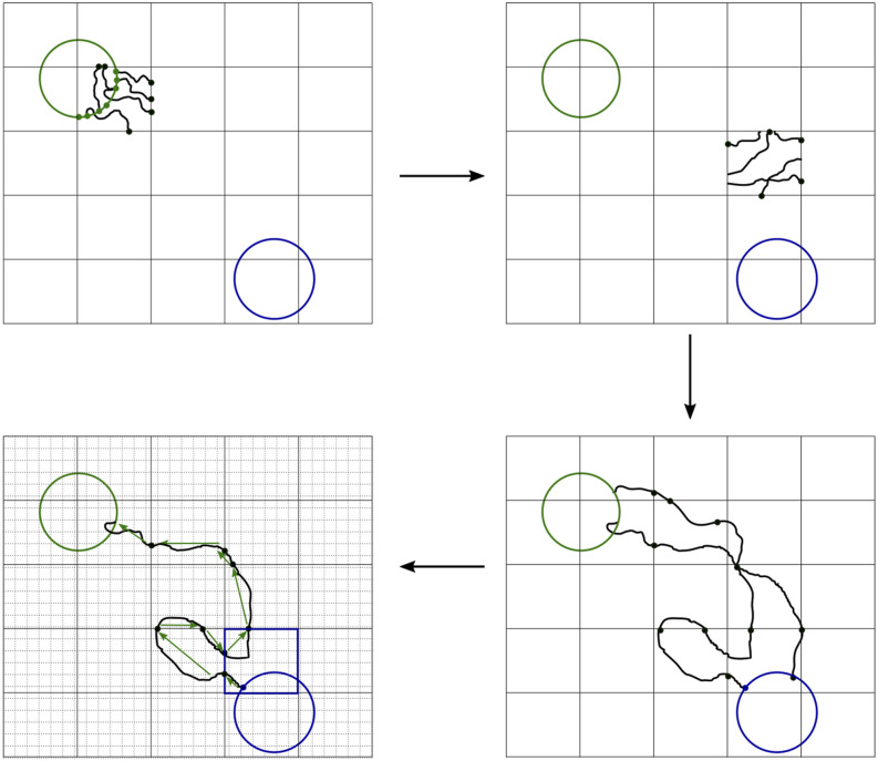
Figure 1 shows how the algorithm samples the ensemble of reactive trajectories in a piecewise fashion and how they are reconstructed.
FIG. 1.
Schematic of the algorithm. (upper left) Define the metastable states and the strata (black grid) and initialize the data structures (step 1). In the example shown, trajectories are initialized from the upper left metastable state boundary, so the last metastable state visited is known. (upper right) In each stratum, draw configurations from γij(dx), save pointers to the associated γij(dx) elements, and then run unbiased dynamics from these configurations until the trajectories exit the stratum (steps 2b and 2c). A single example stratum is shown. (lower right) As the simulation progresses, each point in γij(dx) may give rise to segments of reactive or unreactive trajectories. Save the collective variable values associated with these trajectory segments (step 2d). (lower left) When a reactive or unreactive trajectory is realized (i.e., a trajectory segment enters a metastable state), trace back from pointer to pointer to determine the sequences of strata and collective variable grid sites (gray grid) visited (step 3). Use these to increment unnormalized statistics with appropriate weights (steps 3a–3c). Note that the collective variable grid sites and the strata need not coincide.
IV. NUMERICAL RESULTS
We demonstrate our method by analyzing the C7ax → C7eq transition of the alanine dipeptide (N-acetyl-alanyl-N′-methylamide) in vacuum. The peptide is represented by the CHARMM36m force field.41–43 The simulations are performed at 300 K with the SD (stochastic dynamics) integrator44 in GROMACS 5.1.4;45 LINCS was used to constrain the lengths of bonds to hydrogen atoms; the step size was 1 fs, and the friction coefficient was 10 ps−1. We used PLUMED 2.346,47,48 to extract collective variables; simulations were terminated when walkers left their strata as determined by the PLUMED COMMITTOR function.
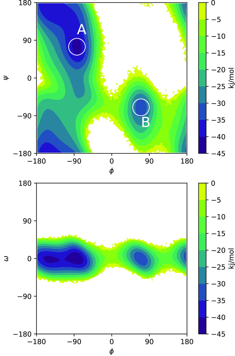
The metastable states and strata are defined in terms of the ϕ and ψ dihedral angles. The metastable states are taken to be circles of radius 20° around (ϕ, ψ) = (−83°, 75°) and (70°, −70°), which correspond to the minima of the potential of mean force determined below. The system was initialized from preliminary trajectories that were generated by using Steered Transition Path Sampling (STePS)40 to drive the system from each metastable state to the other. STePS builds up trajectories by repeatedly shooting bursts of short segments and then preferentially selecting those that make forward progress for continuation. Trajectories were initialized from points in the equilibrium ensemble within each metastable state, and progress was measured by the distance to the center of the other metastable state. The segment length was 1 ps, and the bias threshold was 0.75 (i.e., forward trajectories are selected with a probability of 0.75 or their probability estimated from the burst, whichever is higher). Initially, 10 trajectories were released in each burst; subsequently, we varied the number with the progress distance such as to expect two forward segments in each burst based on statistics of the previous run. We do not use the statistics to correct for the STePS bias—i.e., each reactive trajectory is weighted equally.
The strata form a partition of unity; their centers are at (−7 + 2n)30° for integer n ∈ [1, 6], and their widths are 100°, so they overlap 40° both ways, and the strata wrap around to enforce periodicity. We release 10 walkers in every stratum in each iteration and run each iteration until all 10 walkers exit their stratum. The collective variables ϕ and ψ and their increments are saved every 100 fs. The lag time used to compute the increments [τ in (8)] was 2 ps. The simulation is run until we see at least 1000 crossings in each direction between the metastable states, i.e., walkers that cross from j ≤ K to j > K and the other way. We used a burn-in period of L′ = 100 iterations. The full simulation was ∼140 × 106 steps. Although we stratify in ϕ and ψ, we can project the results onto other variables as well, and we also consider ω (Fig. 2). Statistics are accumulated for 50 values of each dihedral angle.
FIG. 2.
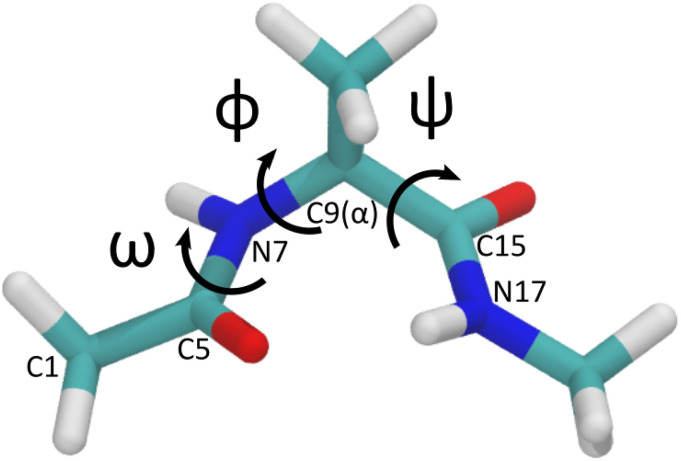
Alanine dipeptide with the three dihedral angles labeled: ϕ [C5–N7–C9(α)–C15], ψ [N7–C9(α)–C15–N17], and ω [C1–C5–N7–C9(α)]. Colors are cyan for carbon, blue for nitrogen, white for hydrogen, and red for oxygen.
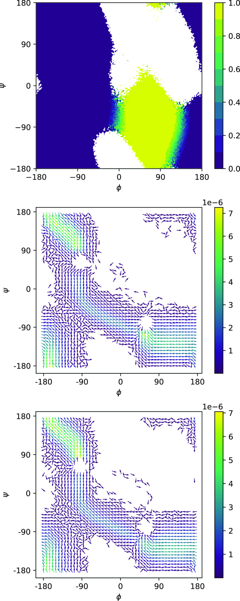
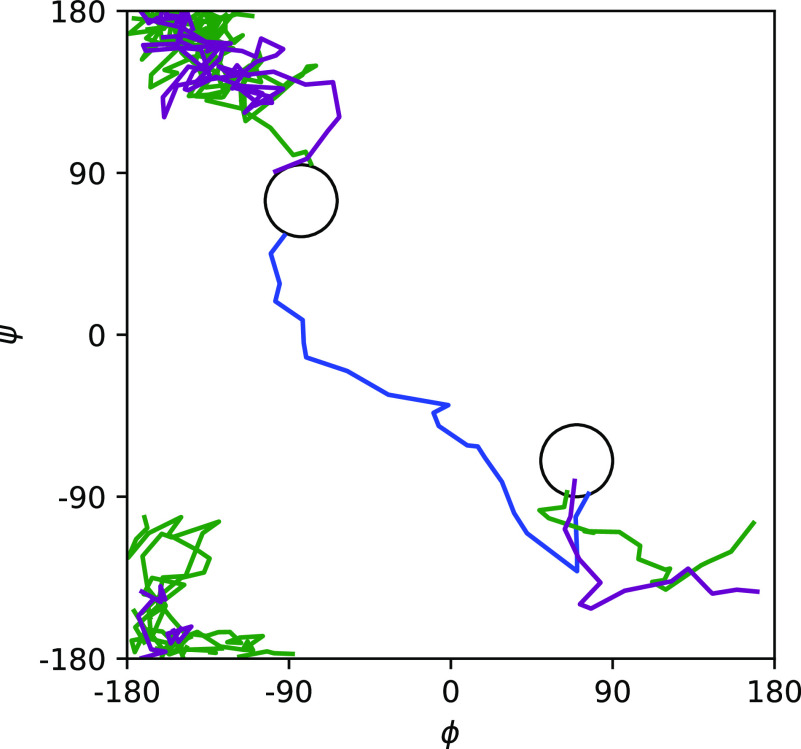
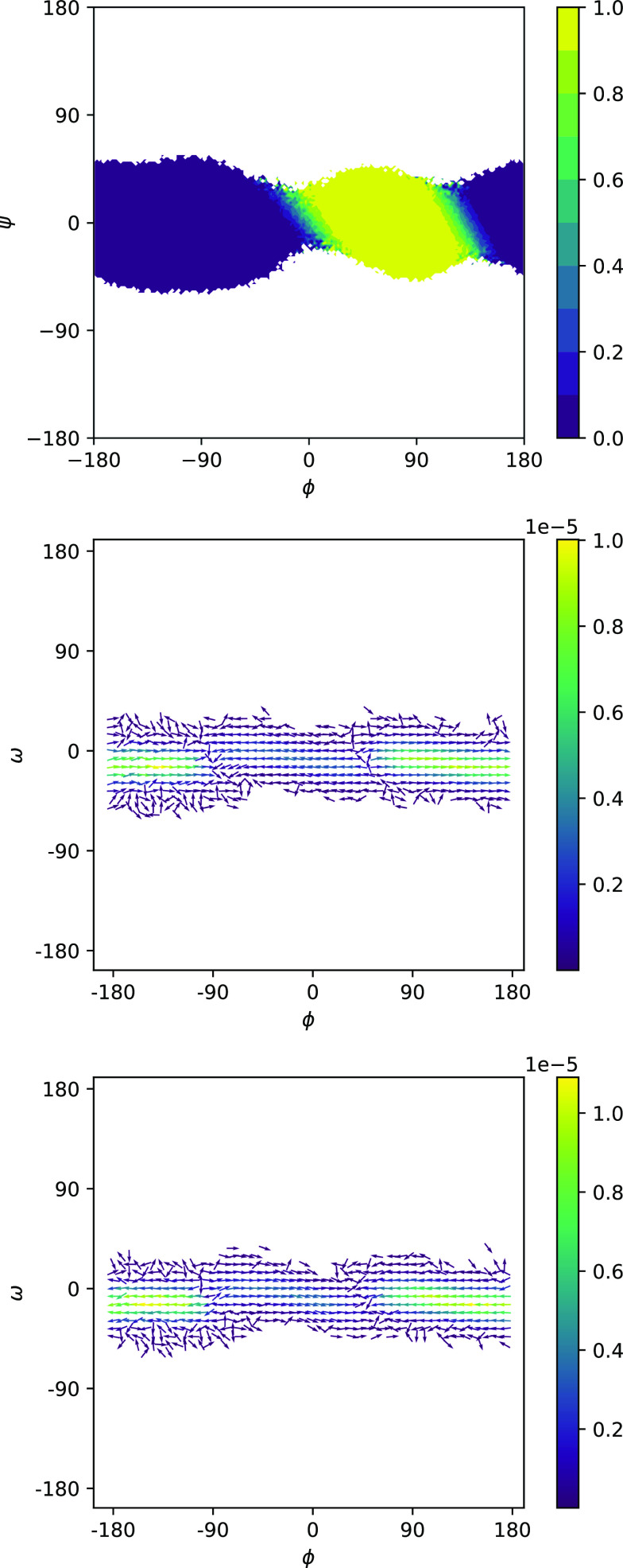
Potentials of mean force (PMFs) computed by NEUS are shown in Fig. 3. In Fig. 4, we show the forward committor and the A → B and B → A currents in the ϕψ-plane. We can see the clear existence of two main pathways, one of which cuts diagonally across the middle and one of which cuts across the upper left and lower right corners. Three representative trajectories consistent with the pathways are shown in Fig. 5. In Fig. 6, we show the committor and currents in the ϕω-plane. We observe a diagonal structure in these plots that is consistent with coupling between distortion of the peptide plane and ϕ noted previously49.
FIG. 3.
Potentials of mean force computed from the NEUS simulations: projections on (top) ϕ and ψ and (bottom) ϕ and ω. The stable states are marked with white circles on the top plot.
FIG. 4.
Committor (top) and forward (middle) and backward (bottom) reactive currents for the C7ax → C7eq transition of the alanine dipeptide, plotted on the ϕψ-plane.
FIG. 5.
Example trajectories plotted on the ϕψ-plane. The circles mark the metastable states.
FIG. 6.
Committor (top) and forward (middle) and backward (bottom) reactive currents for the C7ax → C7eq transition of the alanine dipeptide, plotted on the ϕω-plane. For the reactive currents, only grid points with data from at least five trajectories are shown.
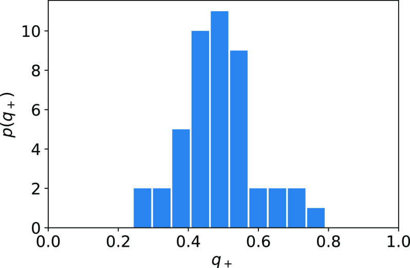
To assess the accuracy of our committor estimates, we compute the committor as a function of all three dihedral angles (not shown), select configurations predicted to have , and evaluate their committors by shooting 20 independent simulations from each configuration. The resulting histogram of values (Fig. 7) is peaked at q+ ≈ 0.5, as desired. To characterize the convergence of the committor estimates, we compute the backward committor and plot , which should be close to zero for this system (Figs. S1 and S2); the deviation provides an indication of the numerical error. We see that after 250 crossings between the metastable states, the error overall is small, with the largest deviations in regions with high free energy close to where . These deviations decrease with additional crossings.
FIG. 7.
Histogram of committors computed by shooting for 137 structures predicted to have for the reaction from A to B. 20 independent simulations were used for each configuration.
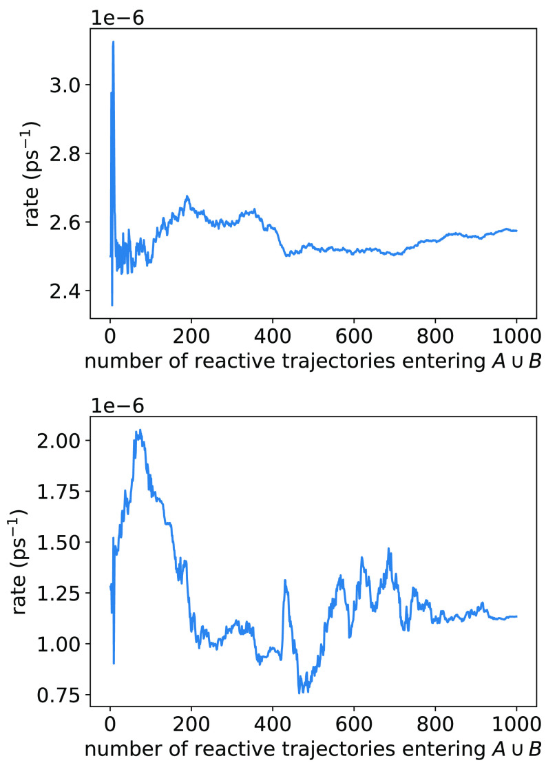
To assess the reactive current estimates, we compute the rate as a function of the number of crossings two ways. First, we directly sum the flux into B,26,27
| (22) |
where is the number of reactive trajectories that enter B from stratum j, Tj is the total time simulated in that stratum, and the sum over j ≤ K selects for contributions from trajectories that were last in A. Second, we sum the reactive currents that cross a dividing surface S,
| (23) |
where is the unit vector normal to S and ΔS is a differential element with the same dimension as S. Since the collective variable space is periodic, there are two pathways, and we average over a set of surfaces for each. Specifically, we use vertical lines in the ϕψ plots: (i) ϕ = (−57.6 + 7.2n)° for integer n in [0, 15], which cut through the middle of Fig. 4, and (ii) ϕ = (−172.8 + 7.2n)° for integer n in [0, 9] and [37, 49], which line the left- and right-hand sides of Fig. 4.
The two estimates are about a factor of two different from each other (Fig. 8); we also obtain a direct estimate of 1.4 × 10⁻⁶ ps−1 from an unbiased trajectory of length 2.5 µs. We consider the three estimates to be at good agreement, given that the rate can be a very challenging statistic to converge to even its order of magnitude. We expect (22) to be most precise (as evidenced by the scale of fluctuations in Fig. 8) and recommend its use; we consider (23) only as a means of validating the reactive currents. That said, we can use the currents to obtain the fluxes associated with each of the pathways. We find them to be RTPT = 4.6 × 10⁻⁷ ps−1 for the pathway that crosses ϕ = 0° and RTPT = 8.1 × 10⁻⁷ ps−1 for the pathway that crosses ϕ = 180°.
FIG. 8.
Rates computed directly from the flux into B (top) and by integrating the reactive currents (bottom). An equal number of crossings between metastable states each way is used for each point on the horizontal axis.
To further assess the reactive currents, we also compute (Fig. S3). We expect this sum to be close to but not exactly equal to zero, given that the integrator is underdamped. We see that this is the case, with the only significant deviations close to the metastable states. Put together, these results validate the method.
V. CONCLUSIONS
In this paper, we investigated the computation of committors and reactive currents with trajectory stratification. The fundamental challenge is that these quantities require knowledge of the metastable states in which trajectories begin and end, but this information cannot be obtained directly from most walkers within the simulation. To address this issue, we store the collective variable values visited by each walker and the associated collective variable increments sampled, as well as a pointer to the previous walker. This enables us to reconstruct the sequence of walkers that gave rise to a trajectory once it reaches a metastable state, despite the fact that the number of trajectories to which a single walker can contribute grows exponentially with the number of walkers that follow it. The current work builds on previous trajectory stratification studies that showed that computation of the rate requires separating the ensemble of trajectories based on the metastable state in which they originate.26,27 As in previous trajectory stratification studies, the results are exact in the limit of infinite sampling in contrast to MSMs and DGA.
Although we demonstrated the approach with NEUS, it is general and can be applied to other algorithms that sample trajectory segments.18–24,30 By the same token, we focused on a simple numerical example that permits validation of the results. Extending the approach to more complex systems should be straightforward so long as collective variables that enable an efficient stratification and the accumulation of statistics can be identified. This challenge is system specific although methods for facilitating the selection of collective variables based on simulation data exist (e.g., Refs. 1 and 10). In the case of NEUS, the most significant challenge may be that the lists representing γij(dx) can become large (up to 5500 elements in the present example). Although this issue has not been limiting for complex systems treated to date,50 it is an important practical consideration that we leave for future work.
SUPPLEMENTARY MATERIAL
See the supplementary material for justification of (8), committor convergence plots, and sums of forward and backward reactive currents.
ACKNOWLEDGMENTS
The authors wish to thank Chatipat Lorpaiboon and John Strahan for useful discussions and critical readings of the manuscript. This work was supported by the National Institutes of Health (Award No. R35 GM136381) and the National Science Foundation (Award No. DMS-2054306).
AUTHOR DECLARATIONS
Conflict of Interest
The authors have no conflicts to disclose.
DATA AVAILABILITY
Data sharing is not applicable to this article as no new data were created or analyzed in this study.
REFERENCES
- 1.Ma A. and Dinner A. R., “Automatic method for identifying reaction coordinates in complex systems,” J. Phys. Chem. B 109, 6769–6779 (2005). 10.1021/jp045546c [DOI] [PubMed] [Google Scholar]
- 2.Vanden-Eijnden E., “Transition path theory,” in Computer Simulations in Condensed Matter Systems: From Materials to Chemical Biology Volume 1, edited by Ferrario M., Ciccotti G., and Binder K. (Springer Berlin Heidelberg, Berlin, Heidelberg, 2006), pp. 453–493. [Google Scholar]
- 3.E W. and Vanden-Eijnden E., “Towards a theory of transition paths,” J. Stat. Phys. 123, 503 (2006). 10.1007/s10955-005-9003-9 [DOI] [Google Scholar]
- 4.Metzner P., Schütte C., and Vanden-Eijnden E., “Illustration of transition path theory on a collection of simple examples,” J. Chem. Phys. 125, 084110 (2006). 10.1063/1.2335447 [DOI] [PubMed] [Google Scholar]
- 5.Noé F., Schütte C., Vanden-Eijnden E., Reich L., and Weikl T. R., “Constructing the equilibrium ensemble of folding pathways from short off-equilibrium simulations,” Proc. Natl. Acad. Sci. U. S. A. 106, 19011–19016 (2009). 10.1073/pnas.0905466106 [DOI] [PMC free article] [PubMed] [Google Scholar]
- 6.Bowman G. R., Pande V. S., and Noé F., An Introduction to Markov State Models and Their Application to Long Timescale Molecular Simulation (Springer Science & Business Media, 2013), Vol. 797. [Google Scholar]
- 7.Wu H., Nüske F., Paul F., Klus S., Koltai P., and Noé F., “Variational Koopman models: Slow collective variables and molecular kinetics from short off-equilibrium simulations,” J. Chem. Phys. 146, 154104 (2017). 10.1063/1.4979344 [DOI] [PubMed] [Google Scholar]
- 8.Buchete N.-V. and Hummer G., “Coarse master equations for peptide folding dynamics,” J. Phys. Chem. B 112, 6057–6069 (2008). 10.1021/jp0761665 [DOI] [PubMed] [Google Scholar]
- 9.Thiede E. H., Giannakis D., Dinner A. R., and Weare J., “Galerkin approximation of dynamical quantities using trajectory data,” J. Chem. Phys. 150, 244111 (2019). 10.1063/1.5063730 [DOI] [PMC free article] [PubMed] [Google Scholar]
- 10.Strahan J., Antoszewski A., Lorpaiboon C., Vani B. P., Weare J., and Dinner A. R., “Long-time-scale predictions from short-trajectory data: A benchmark analysis of the trp-cage miniprotein,” J. Chem. Theory Comput. 17, 2948–2963 (2021). 10.1021/acs.jctc.0c00933 [DOI] [PMC free article] [PubMed] [Google Scholar]
- 11.Russo J. D., Copperman J., Aristoff D., Simpson G., and Zuckerman D. M., “Unbiased estimation of equilibrium, rates, and committors from Markov state model analysis,” arXiv:2105.13402 (2021).
- 12.Elber R., Bello-Rivas J. M., Ma P., Cardenas A., and Fathizadeh A., “Calculating iso-committor surfaces as optimal reaction coordinates with milestoning,” Entropy 19, 219 (2017). 10.3390/e19050219 [DOI] [PMC free article] [PubMed] [Google Scholar]
- 13.Faradjian A. K. and Elber R., “Computing time scales from reaction coordinates by milestoning,” J. Chem. Phys. 120, 10880–10889 (2004). 10.1063/1.1738640 [DOI] [PubMed] [Google Scholar]
- 14.Elber R., “Milestoning: An efficient approach for atomically detailed simulations of kinetics in biophysics,” Annu. Rev. Biophys. 49, 69–85 (2020). 10.1146/annurev-biophys-121219-081528 [DOI] [PubMed] [Google Scholar]
- 15.Dellago C., Bolhuis P. G., Csajka F. S., and Chandler D., “Transition path sampling and the calculation of rate constants,” J. Chem. Phys. 108, 1964–1977 (1998). 10.1063/1.475562 [DOI] [Google Scholar]
- 16.Dellago C., Bolhuis P. G., and Chandler D., “Efficient transition path sampling: Application to Lennard-Jones cluster rearrangements,” J. Chem. Phys. 108, 9236–9245 (1998). 10.1063/1.476378 [DOI] [Google Scholar]
- 17.Dellago C., Bolhuis P. G., Geissler P. L. et al. , “Transition path sampling,” Adv. Chem. Phys. 123, 1 (2002). 10.1002/0471231509.ch1 [DOI] [Google Scholar]
- 18.Huber G. A. and Kim S., “Weighted-ensemble Brownian dynamics simulations for protein association reactions,” Biophys. J. 70, 97–110 (1996). 10.1016/s0006-3495(96)79552-8 [DOI] [PMC free article] [PubMed] [Google Scholar]
- 19.Zhang B. W., Jasnow D., and Zuckerman D. M., “Efficient and verified simulation of a path ensemble for conformational change in a united-residue model of calmodulin,” Proc. Natl. Acad. Sci. U. S. A. 104, 18043–18048 (2007). 10.1073/pnas.0706349104 [DOI] [PMC free article] [PubMed] [Google Scholar]
- 20.Zuckerman D. M. and Chong L. T., “Weighted ensemble simulation: Review of methodology, applications, and software,” Annu. Rev. Biophys. 46, 43–57 (2017). 10.1146/annurev-biophys-070816-033834 [DOI] [PMC free article] [PubMed] [Google Scholar]
- 21.Bolhuis P. G., “Transition-path sampling of β-hairpin folding,” Proc. Natl. Acad. Sci. U. S. A. 100, 12129–12134 (2003). 10.1073/pnas.1534924100 [DOI] [PMC free article] [PubMed] [Google Scholar]
- 22.van Erp T. S., Moroni D., and Bolhuis P. G., “A novel path sampling method for the calculation of rate constants,” J. Chem. Phys. 118, 7762–7774 (2003). 10.1063/1.1562614 [DOI] [Google Scholar]
- 23.Allen R. J., Warren P. B., and ten Wolde P. R., “Sampling rare switching events in biochemical networks,” Phys. Rev. Lett. 94, 018104 (2005). 10.1103/PhysRevLett.94.018104 [DOI] [PubMed] [Google Scholar]
- 24.Allen R. J., Valeriani C., and ten Wolde P. R., “Forward flux sampling for rare event simulations,” J. Phys.: Condens. Matter 21, 463102 (2009). 10.1088/0953-8984/21/46/463102 [DOI] [PubMed] [Google Scholar]
- 25.Warmflash A., Bhimalapuram P., and Dinner A. R., “Umbrella sampling for nonequilibrium processes,” J. Chem. Phys. 127, 154112 (2007). 10.1063/1.2784118 [DOI] [PubMed] [Google Scholar]
- 26.Dickson A., Warmflash A., and Dinner A. R., “Separating forward and backward pathways in nonequilibrium umbrella sampling,” J. Chem. Phys. 131, 154104 (2009). 10.1063/1.3244561 [DOI] [PubMed] [Google Scholar]
- 27.Vanden-Eijnden E. and Venturoli M., “Exact rate calculations by trajectory parallelization and tilting,” J. Chem. Phys. 131, 044120 (2009). 10.1063/1.3180821 [DOI] [PubMed] [Google Scholar]
- 28.Dickson A. and Dinner A. R., “Enhanced sampling of nonequilibrium steady states,” Annu. Rev. Phys. Chem. 61, 441–459 (2010). 10.1146/annurev.physchem.012809.103433 [DOI] [PubMed] [Google Scholar]
- 29.Dinner A. R., Thiede E. H., Van Koten B., and Weare J., “Stratification as a general variance reduction method for Markov chain Monte Carlo,” SIAM/ASA J. Uncertainty Quantif. 8, 1139–1188 (2020). 10.1137/18m122964x [DOI] [PMC free article] [PubMed] [Google Scholar]
- 30.Bello-Rivas J. M. and Elber R., “Exact milestoning,” J. Chem. Phys. 142, 094102 (2015). 10.1063/1.4913399 [DOI] [PMC free article] [PubMed] [Google Scholar]
- 31.Bhatt D., Zhang B. W., and Zuckerman D. M., “Steady-state simulations using weighted ensemble path sampling,” J. Chem. Phys. 133, 014110 (2010). 10.1063/1.3456985 [DOI] [PMC free article] [PubMed] [Google Scholar]
- 32.Dinner A. R., Mattingly J. C., Tempkin J. O. B., Van Koten B., and Weare J., “Trajectory stratification of stochastic dynamics,” SIAM Rev. 60, 909–938 (2018). 10.1137/16m1104329 [DOI] [PMC free article] [PubMed] [Google Scholar]
- 33.Lorpaiboon C., Weare J., and Dinner A. R., “Augmented transition path theory for sequences of events” arXiv:2205.05067 (2022). [DOI] [PMC free article] [PubMed]
- 34.Metzner P., Schütte C., and Vanden-Eijnden E., “Transition path theory for Markov jump processes,” Multiscale Model. Simul. 7, 1192–1219 (2009). 10.1137/070699500 [DOI] [Google Scholar]
- 35.Torrie G. M. and Valleau J. P., “Nonphysical sampling distributions in Monte Carlo free-energy estimation: Umbrella sampling,” J. Comput. Phys. 23, 187–199 (1977). 10.1016/0021-9991(77)90121-8 [DOI] [Google Scholar]
- 36.Pangali C., Rao M., and Berne B. J., “A Monte Carlo simulation of the hydrophobic interaction,” J. Chem. Phys. 71, 2975–2981 (1979). 10.1063/1.438701 [DOI] [Google Scholar]
- 37.Frenkel D. and Smit B., Understanding Molecular Simulation: From Algorithms to Applications (Elsevier, 2001). [Google Scholar]
- 38.Thiede E. H., Van Koten B., Weare J., and Dinner A. R., “Eigenvector method for umbrella sampling enables error analysis,” J. Chem. Phys. 145, 084115 (2016). 10.1063/1.4960649 [DOI] [PMC free article] [PubMed] [Google Scholar]
- 39.Dickson A., Warmflash A., and Dinner A. R., “Nonequilibrium umbrella sampling in spaces of many order parameters,” J. Chem. Phys. 130, 074104 (2009). 10.1063/1.3070677 [DOI] [PubMed] [Google Scholar]
- 40.Guttenberg N., Dinner A. R., and Weare J., “Steered transition path sampling,” J. Chem. Phys. 136, 234103 (2012). 10.1063/1.4724301 [DOI] [PubMed] [Google Scholar]
- 41.MacKerell A. D., Bashford D., Bellott M., Dunbrack R. L., Evanseck J. D., Field M. J., Fischer S., Gao J., Guo H., Ha S., Joseph-McCarthy D., Kuchnir L., Kuczera K., Lau F. T. K., Mattos C., Michnick S., Ngo T., Nguyen D. T., Prodhom B., Reiher W. E., Roux B., Schlenkrich M., Smith J. C., Stote R., Straub J., Watanabe M., Wiórkiewicz-Kuczera J., Yin D., and Karplus M., “All-atom empirical potential for molecular modeling and dynamics studies of proteins,” J. Phys. Chem. B 102, 3586–3616 (1998). 10.1021/jp973084f [DOI] [PubMed] [Google Scholar]
- 42.Best R. B., Zhu X., Shim J., Lopes P. E. M., Mittal J., Feig M., and MacKerell A. D., “Optimization of the additive CHARMM all-atom protein force field targeting improved sampling of the backbone ϕ, ψ and side-chain χ1 and χ2 dihedral angles,” J. Chem. Theory Comput. 8, 3257–3273 (2012). 10.1021/ct300400x [DOI] [PMC free article] [PubMed] [Google Scholar]
- 43.Huang J., Rauscher S., Nawrocki G., Ran T., Feig M., de Groot B. L., Grubmüller H., and A. D. MacKerell, Jr., “CHARMM36m: An improved force field for folded and intrinsically disordered proteins,” Nat. Methods 14, 71–73 (2017). 10.1038/nmeth.4067 [DOI] [PMC free article] [PubMed] [Google Scholar]
- 44.Goga N., Rzepiela A. J., De Vries A. H., Marrink S. J., and Berendsen H. J. C., “Efficient algorithms for Langevin and DPD dynamics,” J. Chem. Theory Comput. 8, 3637–3649 (2012). 10.1021/ct3000876 [DOI] [PubMed] [Google Scholar]
- 45.Abraham M. J., Murtola T., Schulz R., Páll S., Smith J. C., Hess B., and Lindahl E., “GROMACS: High performance molecular simulations through multi-level parallelism from laptops to supercomputers,” SoftwareX 1-2, 19–25 (2015). 10.1016/j.softx.2015.06.001 [DOI] [Google Scholar]
- 46.Bonomi M., Branduardi D., Bussi G., Camilloni C., Provasi D., Raiteri P., Donadio D., Marinelli F., Pietrucci F., Broglia R. A., and Parrinello M., “PLUMED: A portable plugin for free-energy calculations with molecular dynamics,” Comput. Phys. Commun. 180, 1961–1972 (2009). 10.1016/j.cpc.2009.05.011 [DOI] [Google Scholar]
- 47.Tribello G. A., Bonomi M., Branduardi D., Camilloni C., and Bussi G., “PLUMED 2: New feathers for an old bird,” Comput. Phys. Commun. 185, 604–613 (2014). 10.1016/j.cpc.2013.09.018 [DOI] [Google Scholar]
- 48.Bonomi M., Bussi G., Camilloni C., Tribello G. A., Banáš P., Barducci A., Bernetti M., Bolhuis P. G., Bottaro S., Branduardi D., Capelli R., and Carloni P., “Promoting transparency and reproducibility in enhanced molecular simulations,” Nat. Methods 16, 670–673 (2019). 10.1038/s41592-019-0506-8 [DOI] [PubMed] [Google Scholar]
- 49.Bolhuis P. G., Dellago C., and Chandler D., “Reaction coordinates of biomolecular isomerization,” Proc. Natl. Acad. Sci. U. S. A. 97, 5877–5882 (2000). 10.1073/pnas.100127697 [DOI] [PMC free article] [PubMed] [Google Scholar]
- 50.Dickson A., Maienschein-Cline M., Tovo-Dwyer A., Hammond J. R., and Dinner A. R., “Flow-dependent unfolding and refolding of an RNA by nonequilibrium umbrella sampling,” J. Chem. Theory Comput. 7, 2710–2720 (2011). 10.1021/ct200371n [DOI] [PubMed] [Google Scholar]
Associated Data
This section collects any data citations, data availability statements, or supplementary materials included in this article.
Supplementary Materials
See the supplementary material for justification of (8), committor convergence plots, and sums of forward and backward reactive currents.
Data Availability Statement
Data sharing is not applicable to this article as no new data were created or analyzed in this study.


