A Hybrid Epidemic Model to Explore Stochasticity in COVID-19 Dynamics

Abstract

The dynamic nature of the COVID-19 pandemic has demanded a public health response that is constantly evolving due to the novelty of the virus. Many jurisdictions in the USA, Canada, and across the world have adopted social distancing and recommended the use of face masks. Considering these measures, it is prudent to understand the contributions of subpopulations—such as “silent spreaders”—to disease transmission dynamics in order to inform public health strategies in a jurisdiction-dependent manner. Additionally, we and others have shown that demographic and environmental stochasticity in transmission rates can play an important role in shaping disease dynamics. Here, we create a model for the COVID-19 pandemic by including two classes of individuals: silent spreaders, who either never experience a symptomatic phase or remain undetected throughout their disease course; and symptomatic spreaders, who experience symptoms and are detected. We fit the model to real-time COVID-19 confirmed cases and deaths to derive the transmission rates, death rates, and other relevant parameters for multiple phases of outbreaks in British Columbia (BC), Canada. We determine the extent to which SilS contributed to BC’s early wave of disease transmission as well as the impact of public health interventions on reducing transmission from both SilS and SymS. To do this, we validate our model against an existing COVID-19 parameterized framework and then fit our model to clinical data to estimate key parameter values for different stages of BC’s disease dynamics. We then use these parameters to construct a hybrid stochastic model that leverages the strengths of both a time-nonhomogeneous discrete process and a stochastic differential equation model. By combining these previously established approaches, we explore the impact of demographic and environmental variability on disease dynamics by simulating various scenarios in which a COVID-19 outbreak is initiated. Our results demonstrate that variability in disease transmission rate impacts the probability and severity of COVID-19 outbreaks differently in high- versus low-transmission scenarios.

Introduction

Infectious diseases are a significant threat to public health and the global economy (Jones et al. 2008). Some of the most well-known infectious diseases originate from coronaviruses, which are enveloped, positive single-strand RNA viruses in the Coronaviridae family that can infect both humans and other mammals (Huang et al. 2020). The majority of human coronavirus infections are mild, but in the past two decades, the epidemics of severe acute respiratory syndrome (SARS) and Middle East respiratory syndrome (MERS) have caused more than 10,000 cumulative cases (Huang et al. 2020). More recently, the Coronavirus disease 2019 (COVID-19) global pandemic has led to the loss of over 4,000,000 lives and has caused unprecedented disruptions to the economies, societies, and health systems worldwide (WHO 2021).

COVID-19 resembles viral pneumonia, with common symptoms such as fever, dry cough, and fatigue (Huang et al. 2020). Due to the drastic impacts of COVID-19 on global public health, there has been increasing interest in identifying the differing contributions of silent spreaders (SilS) and symptomatic spreaders (SymS) to disease transmission. SilS are individuals who are undiagnosed or never develop symptoms throughout the entire course of an infection, which makes them incapable of experiencing disease-induced mortality. SymS display recognizable clinical symptoms, are diagnosed, and may experience disease-induced mortality in severe cases. Due to the absence of symptoms, SilS transmit the infection unknowingly and are less likely to seek medical attention or self-isolate compared to SymS (Gao et al. 2020).

Transmission heterogeneity has been analyzed in stochastic epidemic models, particularly in relation to the impact of superspreaders (SS) versus nonsuperspreaders (NS) (Althouse et al. 2020; Edholm et al. 2018; Garske and Rhodes 2008; James et al. 2007; Lloyd-Smith et al. 2005; Shakiba et al. 2021). The term “superspreader” refers to those who are capable of transmitting an infection to a disproportionately large number of individuals, whereas the majority of the population would only transmit to a few or none (Stein 2011). This discrepancy can be attributed to behavioral, immunological, and physiological differences in the host, as well as environmental factors such as crowding events (Stein 2011). Many of these stochastic modeling approaches with SS have studied transmission heterogeneity using branching processes (Althouse et al. 2020; Garske and Rhodes 2008; James et al. 2007; Lloyd-Smith et al. 2005). In our previous work, we explore the effects of SS on disease dynamics in MERS and Ebola, using a combination of deterministic and stochastic modeling approaches based on the SEAIR (susceptible, exposed, asymptomatic, infectious, recovered) framework (Edholm et al. 2018; Shakiba et al. 2021). A continuous-time Markov chain (CTMC) model with discrete random variables allowed us to identify the influence of demographic variability, or more specifically, the variability in transitions between states due to disease transmission, recovery, and disease-related deaths (as opposed to environmental variability) (Edholm et al. 2018). Specifically, the increased prevalence of SS in the population is associated with an increased possibility of outbreak and a decrease in the time to outbreak (Edholm et al. 2018). We incorporated time-dependent environmental variability into the disease transmission, developing two alternative models: a time-nonhomogeneous stochastic process (NHP) model with discrete random variables (extension of the CTMC model), and a stochastic differential equation (SDE) model with continuous random variables (Shakiba et al. 2021). Through these previous works, we demonstrated the importance of incorporating stochasticity to more realistically capture the epidemiological dynamics. From the NHP and SDE, we found that increased environmental variability results in more severe, but less frequent outbreaks (Shakiba et al. 2021).

SilS are related to SS in their underestimated potential in disease transmission. The estimated proportion of SilS greatly vary across existing models, depending on the strategies used and the location of interest. Earlier studies in Japan estimated the asymptomatic proportion to range from 17.9 to 30.8% (Mizumoto et al. 2020; Nishiura et al. 2020). In Italy, Giordano et al. have divided the detected and undetected cases across different illness severity levels and estimated the proportion of undetected cases to be 35% (Giordano et al. 2020). Buitrago-Garcia et al., through a systematic review, estimate that 29% of cases remain asymptomatic (95% CI: 23–37%) (Buitrago-Garcia et al. 2020). Despite these existing studies, there has yet to be a model designed to identify the contributions of SilS in British Columbia (BC), Canada. It is important to note that our definition for SilS encapsulates both the undiagnosed and asymptomatic individuals.

Building upon our previous models, we investigate the contributions of SilS versus SymS in BC’s COVID-19 disease dynamics. We seek to determine the extent to which SilS contributed to BC’s early wave of disease transmission as well as the impact that public health interventions had on reducing transmission from both SilS and SymS. To do this, we begin by validating our model against an existing COVID-19 parameterized model to check the degree of similarity between the model outputs. We then split BC’s COVID-19 timeline into two phases based on the public health measures in place, such as the degree of social distancing. With these defined phases, we fit our SEAIR model to clinical data of the number of confirmed infections and deaths over time and estimate key parameter values for different stages of BC’s disease dynamics. These parameters are used to construct stochastic models that help us explore the impacts of demographic and environmental variability on disease dynamics. Importantly, the new stochastic model is a hybrid of the NHP and SDE, which was developed to find a balance between model accuracy and efficiency based on the number of infections in the population at any given time. The new model is applied to the SEAIR framework and includes environmental heterogeneity through a separate time-nonhomogeneous SDE for the disease transmission parameters. While this latter approach has been used by us and others (Allen 2016; Cai et al. 2018; Marion et al. 2000; Shakiba et al. 2021; Truscott and Gilligan 2003; Varughese and Fatti 2008), our hybrid model differs from some of the existing hybrid models with CTMCs and SDEs as these are time-homogeneous processes with constant parameters, and they are often restricted to the SIR framework (Rebuli et al. 2017; Safta et al. 2015; Sazonov et al. 2011). In our new hybrid model, we study the effect of variability in disease transmission as well as the rate at which variations in transmission are returned to their mean value, which is a proxy for the degree of public health policing. We find that variability impacts the probability and severity of COVID-19 outbreaks differently in high- versus low-transmission scenarios.

Mathematical Models

Deterministic Epidemic Model

First, we model the dynamics of SilS and SymS with a system of ordinary differential equations (ODEs). We parameterize the system of ODEs with COVID-19 data in Sect. 4.2. The compartmental diagram for the ODEs can be seen in Fig. 1. The population is divided into two groups, SilS and SymS, according to their response to COVID-19 infection. When individuals in group 1, SilS, become infected, they do not exhibit symptoms (they remain asymptomatic) and the infection is mild, whereas individuals in group 2, SymS, exhibit symptoms and the infection is more serious (possibly resulting in death). The disease stages for both groups include susceptible $S_i$, exposed $E_i$, asymptomatic $A_i$, and recovered $R_i$, where the subscript $i=1$ denotes SilS and $i=2$ denotes SymS. The additional infectious stage $I_2$ is included for SymS. An asymptomatic individual does not have symptoms but can transmit the infection, whereas an infectious individual has symptoms and transmits the infection. Therefore, COVID-19 can be transmitted to susceptible individuals in the population from either SymS or SilS during the asymptotic stages, $A_1$ and $A_2$, or from SymS during the infectious stage $I_2$. Demographic variations unrelated to COVID-19 such as natural births and deaths are excluded from our ODE model and are not expected to play a significant role in population dynamics in this short time.

Fig. 1.

a Compartmental diagram outlining the ODE dynamics. SilS ($i=1$) and SymS ($i=2$) are subdivided into several stages: susceptible, exposed, asymptomatic, infectious, recovered ($S_i,E_i,A_i,I_i,R_i$). The I stage is absent from SilS. Solid arrows denote transitions between stages. Dashed arrows represent the transmission of disease from the A and I stages to the susceptible population, which induces the transition from $S_i$ to $E_i$. Parameters are defined in Table 3. b Our classification of SilS and SymS is based on both diagnosis and symptom development. On the left are SilS individuals who are undetected and possibly never develop symptoms. Meanwhile, on the right are SymS individuals who are detected and develop symptoms

The explicit form of the ODEs is

$$\begin{array}{cc}\hfill {\displaystyle \frac{d{S}_i}{\mathit{dt}}}=& -\left({\displaystyle \frac{{\beta }_1{A}_1}{N}},+,{\displaystyle \frac{{\beta }_2{A}_2}{N}},+,{\displaystyle \frac{{\beta }_3{I}_2}{N}}\right)S_i,i=1,2,\hfill \\ \hfill {\displaystyle \frac{d{E}_i}{\mathit{dt}}}=& \left({\displaystyle \frac{{\beta }_1{A}_1}{N}},+,{\displaystyle \frac{{\beta }_2{A}_2}{N}},+,{\displaystyle \frac{{\beta }_3{I}_2}{N}}\right)S_i-{\alpha }_i{E}_i,i=1,2,\hfill \\ \hfill {\displaystyle \frac{d{A}_i}{\mathit{dt}}}=& {\alpha }_i{E}_i-{\delta }_i{A}_i,i=1,2,\hfill \\ \hfill {\displaystyle \frac{d{I}_2}{\mathit{dt}}}=& {\delta }_2{A}_2-\gamma I_2-\mu I_2,\hfill \\ \hfill {\displaystyle \frac{d{R}_1}{\mathit{dt}}}=& {\delta }_1{A}_1,\hfill \\ \hfill {\displaystyle \frac{d{R}_2}{\mathit{dt}}}=& \gamma I_2.\hfill \end{array}$$

Parameter ${\beta }_1$ is the transmission rate from $A_1$, ${\beta }_2$ from $A_2$, and ${\beta }_3$ from $I_2.$ The total population size is $N=N_1+N_2$, where $N_1=S_1+E_1+A_1+R_1$ is the population size of SilS and $N_2=S_2+A_2+E_2+I_2+R_2$ is the size of SymS.

Disease-related deaths in SymS result in a decrease in the population size of the SymS over time, $d{N}_2/dt=-\mu I_2$ but the population size of SilS remains constant, $N_1(t)=N_1(0).$ The initial conditions are nonnegative with $R_1(0)=0=R_2(0).$

For constant parameter values, a simple expression can be computed for the basic reproduction number in the ODE model by applying the next generation matrix approach (van den Driessche and Watmough 2002; Diekmann et al. 1990). Let $p_1(t)=S_1(t)/N(t)$ be the proportion of susceptible SilS (group 1) and $p_2(t)=S_2(t)/N(t)$ the proportion of susceptible SymS (group 2) at time t. At the beginning of an epidemic, when the population is at the disease-free equilibrium (DFE), $S_1(0)=N_1(0)$ and $S_2(0)=N_2(0)$ with remaining states zero, the basic reproduction number can be defined in terms of the proportions,

$$\begin{array}{c}\hfill {\mathcal{R}}_0=\underset{\mathrm{SilS}}{\underbrace{p_1(0){\displaystyle \frac{{\beta }_1}{{\delta }_1}}}}+\underset{\mathrm{SymS}}{\underbrace{p_2(0)\left({\displaystyle \frac{{\beta }_2}{{\delta }_2}},+,{\displaystyle \frac{{\beta }_3}{\gamma +\mu }}\right)}}.\end{array}$$ 1

For constant parameters, ${\mathcal{R}}_0$ is the sum of two terms, the number of secondary infections generated from SilS and from SymS. The stability of the DFE is achieved if the proportion of the susceptible population in each group reaches a sufficiently small fraction of the population. That is, if the effective reproduction number is reduced to a value less than one,

$$\begin{array}{c}\hfill {\mathcal{R}}_t=p_1(t){\displaystyle \frac{{\beta }_1}{{\delta }_1}}+p_2(t)\left({\displaystyle \frac{{\beta }_2}{{\delta }_2}},+,{\displaystyle \frac{{\beta }_3}{\gamma +\mu }}\right).\end{array}$$ 2

Stochastic Epidemic Models

To account for demographic and environmental variability in the epidemic process, we develop two time-nonhomogeneous stochastic processes. The first model is a Markov chain model with discrete random variables. The discrete changes in the populations at the initiation of an epidemic accurately account for the small numbers of exposed, asymptomatic, and infectious individuals. We refer to this time-nonhomogeneous process as the NHP model. The second model is a system of SDEs with continuous random variables, an approximation of the NHP model when the numbers of exposed, asymptomatic, and infectious individuals are large. We refer to this model as the SDE model. These two models are coupled in a hybrid model that switches from the NHP to the SDE model when infected population sizes are large and has the reverse switch when population sizes are small. The use of a hybrid model incorporates the accuracy of the NHP when population sizes are small and the computational efficiency of the SDE model when sizes are large.

For simplicity, we use the same notation for the random variables in the NHP and SDE models as in the ODE model, i.e., $S_i$, $E_i$, $A_i$, $I_2$, and $R_i$. To account for demographic variability and to ensure a close relationship to the ODE model, we apply the transition rates in the ODE model to define infinitesimal transition probabilities and the corresponding changes in the NHP random variables. Table 1 outlines all of the changes that occur in the NHP model. In particular, the COVID-19 NHP model is based on the 8 discrete changes in Table 1 and their associated transition probabilities. An underlying assumption in the stochastic model with constant parameters is that the time spent in each stage is exponentially distributed.

Table 1.

State transitions and rates for the COVID-19 NHP model with Poisson probabilities $a(t)\Delta t+o(\Delta t)$

Event	Description	Transition	Rate, a(t)
	Infection of $S_i$	$S_i\to S_i-1$
1, 2		$E_i\to E_i+1$	${\displaystyle \frac{S_i}{N}}\left({\beta }_1,(t),A_1,+,{\beta }_2,(t),A_2,+,{\beta }_3,(t),I_2\right)$
	Transition of $E_i$	$E_i\to E_i-1$
3, 4		$A_i\to A_i+1$	${\alpha }_i{E}_i$
	Transition of $A_2$	$A_2\to A_2-1$
5		$I_2\to I_2+1$	${\delta }_2{A}_2$
	Recovery of $A_1$	$A_1\to A_1-1$
6		$R_1\to R_1+1$	${\delta }_1{A}_1$
	Recovery of $I_2$	$I_2\to I_2-1$
7		$R_2\to R_2+1$	$\gamma I_2$
8	Death of $I_2$	$I_2\to I_2-1$	$\mu I_2$

The transition probabilities in Table 1 are used to derive an Itô SDE model with the general form:

$$\begin{array}{c}\hfill dX(t)=\underset{\mathrm{drift}}{\underbrace{F(X(t),t)}}dt+\underset{\mathrm{diffusion}}{\underbrace{G(X(t),t)}}dW(t),X(0)\ge 0,\end{array}$$ 3

where F is the drift vector, G is the diffusion matrix, and W is a vector of independent Wiener processes (Allen et al. 2020, 2008; Shakiba et al. 2021). The diffusion matrix is a $9\times 8$ block diagonal matrix with two matrices associated with SilS or SymS along the diagonal,

$$\begin{array}{c}\hfill G=\left(\begin{array}{cc}{C}_{\mathrm{SilS}}& O\\ O& C_{\mathrm{SymS}}\end{array}\right),\end{array}$$

where matrices $C_{\mathrm{SilS}}$ and $C_{\mathrm{SymS}}$ are, respectively,

$$\begin{array}{c}\hfill \left(\begin{array}{ccc}{\displaystyle -\sqrt{B_1}}& 0& 0\\ {\displaystyle \sqrt{B_1}}& -\sqrt{{\alpha }_1{E}_1}& 0\\ 0& \sqrt{{\alpha }_1{E}_1}& -\sqrt{{\delta }_1{A}_1}\\ 0& 0& \sqrt{{\delta }_1{A}_1}\end{array}\right)\mathrm{and}\\ \hfill \left(\begin{array}{ccccc}{\displaystyle -\sqrt{B_2}}& 0& 0& 0& 0\\ {\displaystyle \sqrt{B_2}}& -\sqrt{{\alpha }_2{E}_2}& 0& 0& 0\\ 0& \sqrt{{\alpha }_2{E}_2}& -\sqrt{{\delta }_2{A}_2}& 0& 0\\ 0& 0& \sqrt{{\delta }_2{A}_2}& -\sqrt{\mu I_2}& -\sqrt{\gamma I_2}\\ 0& 0& 0& 0& \sqrt{\gamma I_2}\end{array}\right).\end{array}$$

The expressions $B_i\equiv B_i(t)={\displaystyle \frac{S_i}{N}}({\beta }_1(t)A_1+{\beta }_2(t)A_2+{\beta }_3(t)I_2)$, $i=1,2$.

The explicit form of the Itô SDE model with demographic variability has the form:

$$\begin{array}{cc}\hfill d{S}_1=& {\displaystyle -\left({\displaystyle \frac{{\beta }_1(t)A_1}{N}},+,{\displaystyle \frac{{\beta }_2(t)A_2}{N}},+,{\displaystyle \frac{{\beta }_3(t)I_2}{N}}\right)S_{1}dt-\sqrt{B_1}d{W}_{11}(t),}\hfill \\ \hfill d{E}_1=& \left(\left({\displaystyle \frac{{\beta }_1(t)A_1}{N}},+,{\displaystyle \frac{{\beta }_2(t)A_2}{N}},+,{\displaystyle \frac{{\beta }_3(t)I_2}{N}}\right),S_1,-,{\alpha }_1,E_1\right)dt\hfill \\ \hfill & {\displaystyle +\sqrt{B_1}d{W}_{11}(t)-\sqrt{{\alpha }_1{E}_1}d{W}_{12}(t),}\hfill \\ \hfill d{A}_1=& ({\alpha }_1{E}_1-{\delta }_1{A}_1)dt+\sqrt{{\alpha }_1{E}_1}d{W}_{12}(t)-\sqrt{{\delta }_1{A}_1}d{W}_{13}(t),\hfill \\ \hfill d{R}_1=& {\delta }_1{A}_{1}dt+\sqrt{{\delta }_1{A}_1}d{W}_{13}(t),\hfill \\ \hfill d{S}_2=& {\displaystyle -\left({\displaystyle \frac{{\beta }_1(t)A_1}{N}},+,{\displaystyle \frac{{\beta }_2(t)A_2}{N}},+,{\displaystyle \frac{{\beta }_3(t)I_2}{N}}\right)S_{2}dt-\sqrt{B_2}d{W}_{21}(t),}\hfill \\ \hfill d{E}_2=& \left(\left({\displaystyle \frac{{\beta }_1(t)A_1}{N}},+,{\displaystyle \frac{{\beta }_2(t)A_2}{N}},+,{\displaystyle \frac{{\beta }_3(t)I_2}{N}}\right),S_2,-,{\alpha }_2,E_2\right)dt\hfill \\ \hfill & {\displaystyle +\sqrt{B_2}d{W}_{21}(t)-\sqrt{{\alpha }_2{E}_2}d{W}_{22}(t),}\hfill \\ \hfill d{A}_2=& ({\alpha }_2{E}_2-{\delta }_2{A}_2)dt+\sqrt{{\alpha }_2{E}_2}d{W}_{22}(t)-\sqrt{{\delta }_2{A}_2}d{W}_{23}(t),\hfill \\ \hfill d{I}_2=& ({\delta }_2{A}_2-\gamma I_2-\mu I_2)dt+\sqrt{{\delta }_2{A}_2}d{W}_{23}(t)-\sqrt{\mu I_2}d{W}_{24}(t)-\sqrt{\gamma I_2}d{W}_{25}(t),\hfill \\ \hfill d{R}_2=& \gamma I_{2}dt+\sqrt{\gamma I_2}d{W}_{25}(t).\hfill \end{array}$$ 4

The 9 SDEs have a total 8 independent Wiener processes, $W_{1j}$, $j=1,2,3$ and $W_{2j}$, $j=1,2,3,4,5$, corresponding to the number of events in Table 1.

Environmental variability is included in the stochastic models through the transmission rates, ${\beta }_i(t)$. Environmental variability may be a result of contacts or behavior of the population due to government restrictions imposed on social distancing or on face mask use or from external factors such as temperature or humidity that directly impact transmission. Therefore, environmental variability is modeled by time-dependent, continuous random variables ${\beta }_i(t)$, $i=1,2,3$, through the Itô SDE as

$$\begin{array}{c}\hfill d{\beta }_i(t)=r({\overline{\beta }}_i-{\beta }_i(t))+{\sigma }_i\sqrt{{\beta }_i(t)}dW(t),{\beta }_i(0)={\overline{\beta }}_i,i=1,2,3.\end{array}$$ 5

The values of ${\overline{\beta }}_i$, $i=1,2,3$ are the estimated constant transmission rates from the ODE model in Sect. 4.2. Parameter r is the rate of return to the value ${\overline{\beta }}_i$ and parameter ${\sigma }_i$ is the amount of variability about this value. The Itô SDE (5) is known as a Cox–Ingersoll–Ross (CIR) process (Iacus 2009). The CIR process has nonnegative sample paths and an asymptotic gamma distribution with constant mean ${\overline{\beta }}_i$ and variance ${\overline{\beta }}_i{\sigma }_i^2/(2r)$ (Allen 2016; Shakiba et al. 2021). The coefficient of variation (CV) of the asymptotic gamma probability density function equals

$$\begin{array}{c}\hfill CV={\displaystyle \frac{{\sigma }_i}{\sqrt{2r{\overline{\beta }}_i}}}\mathrm{and}{\sigma }_i=CV\sqrt{2r{\overline{\beta }}_i}.\end{array}$$ 6

The effects of environmental variability on several COVID-19 epidemic outcomes are explored in Sect. 4.4 through a range of values for the two parameters r and CV. If $r=CV=0$, then there is no environmental variability. Therefore, we chose $CV=0.5,1,1.25$ to encompass a large range of environmental variability and values of $r=0.1,0.2,0.5,1$ days${}^{-1}$ to measure the response rate for return to the mean. For example, $r=0.1$ is an average return of 10 days, whereas $r=1$ is 1 day.

The NHP model accurately records the discrete events in the random variables when population sizes are small. However, as population sizes increase, so does the frequency of the discrete events, resulting in large computational times. To alleviate these computational issues, we develop a hybrid model to ensure the accuracy of the NHP model for small population sizes and the computational expediency of the SDE model for large population sizes (2). A hybrid approach has often been used in practice in epidemic models and in chemical reaction models, where in the latter models the SDE formulation is referred to as the chemical Langevin equation (Duncan et al. 2016; Gillespie 2000; Rebuli et al. 2017; Safta et al. 2015; Salis and Kaznessis 2005; Sazonov et al. 2011). When consistently formulated, the SDE model (4)–(5) approximates the NHP dynamics for large population sizes (Allen et al. 2020; Allen 2017; Allen and Allen 2003). To ensure the SDE dynamics follow closely those of the NHP, the SDE model is modified slightly so that the transition rates and the sample paths of the SDE are nonnegative (Allen et al. 2020; Cresson and Sonner 2018) (Appendix B).

For $r>0$ and $CV>0$, the transmission parameters ${\beta }_i$, $i=1,2,3$ are continuous random variables modeled by the SDE Cox–Ingersoll–Ross (CIR) process. The ${\beta }_i$ CIR process can be accurately modeled by the Euler–Maruyama method, a discrete-time method. The standard Gillespie algorithm no longer applies to the NHP when parameters ${\beta }_i$ are modeled by the CIR process. Therefore, to be consistent with the discrete-time method used for the ${\beta }_i$ CIR process, we use a Monte Carlo method with the same discrete-time step as in the NHP epidemic model. The value of $\Delta t$ is chosen sufficiently small such that the sum of all transition probabilities $\alpha (t)\Delta t$ in Table 1 is less than one and that the time step yields a good approximation for the NHP model and the CIR process. If these criteria do not hold, there is a break in the computed simulations and the simulations are redone with a smaller time-step until the criteria are satisfied. In particular, the change in time, $\Delta t$, is chosen as 0.0005. The Euler–Maruyama method with the same time step is then applied to the SDE epidemic model. The use of a discrete-time method in the time-nonhomogeneous NHP and SDE epidemic models provides a seamless transition in the hybrid model, when switching between NHP and SDE.

We validated our Monte Carlo method by comparing the model outputs to that of the CTMC using the Gillespie algorithm, with $r=0=CV$, which we previously developed and published (Edholm et al. 2018). Also, in Shakiba et al. (2021), we have shown that our Monte Carlo discrete-time method and Gillespie algorithm are in good agreement in terms of mean, standard deviation, and other outcome measures.

To numerically implement the hybrid model, we define a switch from NHP to SDE when the sum of the infected random variables $I_2+{\sum }_{i=1,2}(E_i+A_i)$ reaches a threshold value, ${\text{Thresh}}_1=100$ and a reverse switch, SDE to NHP, when ${\text{Thresh}}_2=50$. We tested various threshold values to ensure accuracy of the outcomes. For ${\text{Thresh}}_1=100,500,1000$, it was found that the values are not statistically different via one-way ANOVA and t-test comparing 100 versus 1000 (p-value 0.01). All code for this paper is available at Hwang et al. (2022)

Results

Fig. 2.

An outline of our modeling workflow, which involves validation, phase definition, ODE parameter fitting, and stochastic modeling

Validating our Model Through Comparison to Established Italy Dynamics and Data

Before applying our parameter estimation strategy to BC data, we conduct an extensive literature search to identify published models that have taken a similar approach to model COVID-19 in regions with high case counts in early 2020. We select the SIDARTHE model developed by Giordano et al. for COVID-19 in Italy as a source of validation for our model (Giordano et al. 2020). SIDARTHE is a compartmental model that captures individuals in the susceptible, infected, diagnosed, ailing, recognized, threatened, extinct, and healed classes (Giordano et al. 2020). This model is selected for use in our validation step based on the high degree of overlap between the established classes seen in the SIDARTHE and our SEAIR model. However, since our model parameters differ and cannot be directly compared across models, we use ${\mathcal{R}}_0$ as a baseline for comparison in the model validation process. We perform parameter estimation with the dataset of the SIDARTHE model provided by the Italian Ministry of Health/Civil Protection, which contains the number of cases, deaths, and recoveries in Italy (Giordano et al. 2020).

We limit our fitting to days 1–22 of the initial outbreak in Italy, which began on February 20, 2020. Day 22 is approximately two weeks after the first announcement of public health measures, which recommended citizens to perform basic social distancing. A two-week lag period is chosen since a peak in infections occurred after 14–18 days of lockdown, which reflects the time needed for a population to respond to changes in public health regulations (Vinceti et al. 2020). This period is obtained through analyzing changes in cellphone mobility caused by nationally imposed regulations relating to COVID-19 in Italy (Vinceti et al. 2020). A similar strategy is used to define phases of the pandemic in BC. To parameterize the model, we utilize an extensive literature search and techniques of numerical parameter estimation. First, from the literature we define measurable parameters: latent period, duration for the asymptomatic stage, and total population size. Parameters that are unavailable in the literature are obtained through parameter estimation (marked by asterisks in Table 2). We then use Multistart and fmincon programs in MATLAB to get the model-predicted outputs to match with data through nonlinear least squares fitting (Burton et al. 2021; Edholm et al. 2019; Levy et al. 2017). We want to emphasize that our construction of a deterministic ODE model is formulated to capture the underlying behavior of the pandemic rather than exact parameter values. Given the constraints of the pandemic and our focus on exploring the stochastic nature of the model, we used an established approach to estimate the parameters in our model using data. Day 1 describes the day when the first infected symptomatic person is introduced to the population, which corresponds to an initial condition of $I_2(0)=1$. Once we find the best fit, the associated output parameters are taken as our estimations. Figure 3 shows the best fit. The number of people in each phase can be seen in Fig. 11. After parameter estimation, we obtain an ${\mathcal{R}}_0$ of 2.06, which is in close agreement to ${\mathcal{R}}_0$ = 2.38 found by Giordano et al. (2020). This validation gives us confidence to apply our SEAIR model strategy with BC’s data.

Table 2.

Description of the parameter values for the beginning of the COVID-19 outbreak in Italy (Days 1–22). Parameters marked by * are obtained through methods in Sect. 4.1. Parameter $p=p_1(0)=S_1(0)/N(0)$

	Parameter Definition	Italy	Units	Reference
${\overline{\beta }}_1^{\ast }$	SilS mean asymptomatic transmission rate	0.498	Days${}^{-1}$	–
${\overline{\beta }}_2^{\ast }$	SymS mean asymptomatic transmission rate	0.729	Days${}^{-1}$	–
${\overline{\beta }}_3^{\ast }$	SymS mean symptomatic transmission rate	0.0209	Days${}^{-1}$	–
${\alpha }_1^{-1}$	SilS latent period	3.2	Days	Lauer et al. (2020)
${\alpha }_2^{-1}$	SymS latent period	3.2	Days	Lauer et al. (2020)
${\delta }_1^{-1\ast }$	SilS duration of asymptomatic stage	18.8	Days	–
${\delta }_2^{-1}$	SymS duration of asymptomatic stage	2.3	Days	Bi et al. (2020)
${\mu }^{\ast }$	Disease-induced death rate	0.0149	Days${}^{-1}$	–
${\gamma }^{\ast }$	Recovery rate	0.0217	Days${}^{-1}$	–
N	Total population size	60000000	Individuals	Giordano et al. (2020)
$p^{\ast }$	SilS initial fraction in population	0.2018	-	–

Fig. 3.

Scatter plot of data from Italy for days 1–22 and our corresponding model-predicted trend lines for cumulative cases, deaths, and recovered

Fig. 11.

The ODE solution for each variable is plotted, based on best fit parameters for Days 1–22 of Italy COVID-19 dynamics. (Fits to data are shown in Fig. 3)

Uncovering the Contributions of Silent and Symptomatic Spreaders to BC Outbreak Dynamics

Based on our preliminary analysis of the BC data and policy shifts in reaction to COVID-19, we divide the data into two phases that capture the change in disease dynamics associated with introduction of strict provincial regulations (Alyse 2021). Phase I marks the beginning of the outbreak where few regulations are put in place, while Phase II captures a period of strict social distancing (Fig. 4a). The division between the two phases is based on fluctuations in population behavior caused by social distancing guidelines imposed in March 2020. These trends are captured in the Citymapper Mobility Index, which is a mobile application that tracks a city’s public transit activity when compared to a historic baseline (Citymapper 2020). Specifically, we define the end of Phase I to be March 31, 2020, which is two weeks after BC officials declared a provincial state of emergency over the COVID-19 pandemic on March 17th. This can be seen in the sudden drop in transit activity (Fig. 5b), which remains below 20 percent after March 31, 2020 (Fig. 4b) (Citymapper 2020). After the phases are defined, we continue with parameter estimation in BC, allowing certain parameters to change values based on the particular phase (Burton et al. 2021).

Fig. 4.

a Visualization of the two phases of the BC disease dynamics, with Phase I starting at the emergence of COVID-19. We switch to Phase II at Day 60 until Day 109. b Citymapper Mobility Index data for BC, which reports a shift in behavior around March 31st 2020, day 60 in a. c Scatter plots of data from BC for Phases I and II, along with the model-predicted cumulative number of cases, deaths, and recovered individuals. Deaths are minimized in the Phase II fitting strategy which are expected be a more accurate measure of the disease dynamics than cumulative cases when testing rates are low

Fig. 5.

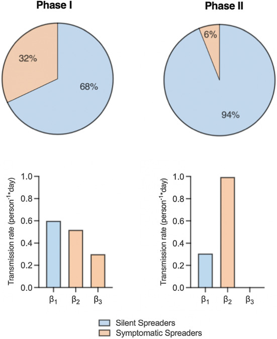
Model-predicted parameterizations of our SEAIR model for Phases I and II of the BC COVID-19 dynamics. Pie charts show the initial proportions of the total population that are SilS versus SymS and the three values for the transmission rates, ${\beta }_1,{\beta }_2$ and ${\beta }_3$. Note, in Phase II ${\beta }_3$ is close to zero

Using the same strategy as we did for Italy, we estimate the Phase I transmission rates (${\beta }_1,{\beta }_2,{\beta }_3$), SymS duration of asymptomatic stage $({\delta }_1^{-1})$, death rate $(\mu )$, recovery rate $(\gamma$), and the SilS fraction (p) with an initial condition of $I_2=1$. To account for continuation between the two phases, the endpoints for Phase I are used as the initial conditions of Phase II and disease-induced deaths from Phase I were removed from the population. Parameters that were assumed to be independent of time were carried over from Phase I to Phase II (${\delta }_1^{-1}$, $\mu$, and $\gamma$ (marked by a single asterisk in Table 3)). Due to the large number of unrecorded cases in BC, we modified the model to minimize deaths in Phase II (Skowronski et al. 2020). Deaths would only result from the severe SymS cases, which are accurately recorded in official data. To account for unrecorded cases, all valid model estimations are greater than or equal to recorded data. The results for fitting Phases I and II in BC are shown in Figs. 4c and 12. There is close agreement between the estimated and actual number of deaths in Phase II, while cases and recoveries are greater than the recorded data due to under-reporting. The number of people in each stage over time during Phase I (13a) and Phase II (13b) can be seen in Fig. 13. Figure 5 summarizes the transmission rates and population fractions in Phases I and II. In both phases, asymptomatic transmission contributes more than symptomatic transmission. Due to the imposed restrictions in Phase II, ${\beta }_3$ nearly reaches zero. In addition, SilS makes up the majority of the population. Interestingly, our model predicts a drastic increase in the SilS proportion when we transition phases. This trend could be associated with under-testing in the population, causing more people to be classified as SilS. It is noteworthy that at this early phase of the pandemic, provincial public health guidelines only recommended testing of individuals showing symptoms associated with COVID-19 infection and testing was not widespread (British Columbia Centre for Disease Control 2021). On average, the number of tests performed daily during Phases I and II capture 0.03% of the population (British Columbia Centre for Disease Control 2021). Analyzing the average daily testing rates for the same date range one year later, we find that the daily tested population has increased to 0.2%. All of our parameter values are recorded in Table 3. For Phase I, we estimate a ${\mathcal{R}}_0=2.75$ using Eq. (1) and parameter values in Table 3. For Phase II, we estimate a ${\mathcal{R}}_{60}=0.94$ at the start of Phase II (day 60) using Eq. (2) and parameter values in Table 3.

Table 3.

Description of the parameter values for Phase I and Phase II of the COVID-19 SEAIR model in BC. Parameters marked by ** were fitted separately in Phases I and II, which were found through methods in Sect. 4.2. Parameters marked by * were fitted in Phase I but assumed to remain the same over time. Parameter $p=p_1(0)=S_1(0)/N(0)$ in Phase I, Eq. (1) or $p=p_1(60)=S_1(60)/N(60)$ in Phase II, Eq. (2)

	Parameter Definition	Phase I	Phase II	Units	Reference
${\overline{\beta }}_1^{\ast \ast }$	SilS mean asymptomatic transmission rate	0.600	0.306	Days${}^{-1}$	–
${\overline{\beta }}_2^{\ast \ast }$	SymS mean asymptomatic transmission rate	0.519	0.995	Days${}^{-1}$	–
${\overline{\beta }}_3^{\ast \ast }$	SymS mean symptomatic transmission rate	0.3	0.000362	Days${}^{-1}$	–
${\alpha }_1^{-1}$	SilS latent period	3.2	3.2	Days	Lauer et al. (2020)
${\alpha }_2^{-1}$	SymS latent period	3.2	3.2	Days	Lauer et al. (2020)
${\delta }_1^{-1\ast }$	SilS duration of asymptomatic stage	2.8	2.8	Days	–
${\delta }_2^{-1}$	SymS duration of asymptomatic stage	2.3	2.3	Days	Bi et al. (2020)
${\mu }^{\ast \ast }$	Disease-induced death rate	0.004	0.00314	Days${}^{-1}$	–
${\gamma }^{\ast }$	Recovery rate	0.075	0.075	Days${}^{-1}$	–
N	Total population size	5110917	5110894	Individuals	[37]
$p^{\ast \ast }$	SilS initial fraction in population	0.6754	0.9379	–	–

Fig. 12.

Log scale scatter plots of data from BC for Phases I and II, along with the model-predicted cumulative number of cases, deaths, and recovered individuals. Deaths are minimized in the Phase II fitting strategy which are expected be a more accurate measure of the disease dynamics than cumulative cases when testing rates are low

Fig. 13.

The ODE solution for each variable is plotted, based on best fit parameters for a Phase I and b Phase II of BC COVID-19 dynamics. (Fits to data are shown in Fig. 4c)

Hybrid Model Numerical Formulation and Comparison

The parameter estimations from our ODE model are used as the baseline for our hybrid stochastic model, which allows us to explore the contributions of demographic and environmental variation to disease dynamics, as in our previous work (Edholm et al. 2018; Shakiba et al. 2021). Figure 7 illustrates the workflow of our hybrid stochastic model, designed to take advantage of the accuracy of the NHP at small population sizes and the efficiency of the SDE at large population sizes.

Fig. 7.

Outline of our hybrid stochastic model’s overall process. We parameterize the model and run the hybrid stochastic model that switches between the NHP and SDE models based on threshold conditions. Model-generated simulations are then used to calculate output measures that capture the probability and severity of COVID-19 outbreak

We previously showed that the SDE is inaccurate at low initial conditions (Shakiba et al. 2021). Therefore, with an initial condition of $I_2(0)=1$, the hybrid model starts by using the NHP. Once the number of infections reaches 100, the hybrid model switches to the SDE until the number of infections drops back below 50, in which case, the hybrid model returns to the NHP. We set the thresholds of 100 and 50 based on repeated errors in the NHP model code when the number of infected individuals increases beyond these points. In particular, we observed errors in the NHP code when the total number of infected individuals reached high levels, as the total sum of all probabilities a(t) $\Delta$ t in Table 1 exceeded one, making the NHP code invalid. The hybrid model’s threshold for switching back from SDE to NHP (a value of 50) is set to be lower than that of switching from NHP to SDE (value of 100) to prevent continuous and unnecessary oscillations between the NHP and SDE models. Other thresholds were explored and did not visibly impact model outcomes. The model exits the loop if cases drop to zero (signifying the end of the pandemic), or if the pandemic lasts beyond our maximum anticipated timeline of 1000 days. After establishing our hybrid model, we compared it to both the NHP and SDE models run separately, using a wide range of initial conditions. The hybrid model code remains error free in cases where the NHP experiences errors, see Fig. 14 in Appendix C.

Fig. 14.

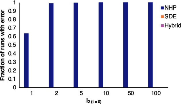
Fraction of runs that output an error for the NHP, SDE, and hybrid stochastic models with number of infections ranging from 1 to 100. The number of initial infected individuals in the population lead to errors in the NHP, but does not effect the SDE or hybrid models

Limitations in the NHP and SDE as standalone models are overcome by combining the two into our hybrid model, which makes use of the advantages of each model. To evaluate the accuracy of the hybrid model, we overlay the sample paths from our model on data and see close alignment between the two (Fig. 6). Using the hybrid stochastic model, we predict the probability and severity of outbreak, which provide valuable insights for public health. Specifically, we estimate the time to outbreak and peak infections, total and peak number of infections, probabilities of outbreak and ICU overload, and the number of death (Fig. 7). By examining how these model-simulated outputs change based on parameters obtained in each phase, we gain valuable insight into how public health policies impact the duration and severity of BC’s COVID-19 pandemic.

Fig. 6.

Sample paths from the hybrid model outputs overlaid on Phase I (a) and II (b) datasets to confirm validity. Each color indicates one sample path

Exploring the Effect of Demographic and Environmental Stochasticity on Phase I and II BC COVID-19 Dynamics

We introduce environmental variability to the hybrid stochastic model through the coefficient of variation (CV) and rate of return (r) (Shakiba et al. 2021). These parameters impact the frequency and amplitude of fluctuations in transmission rates relative to the mean, respectively. The mean transmission rates, which were obtained through parameter fitting in Phases I and II, are expected to changes with public health guidelines imposed on the entire population, including social distancing and masking measures. With relation to disease dynamics, CV impacts the degree to which transmission rates deviate from the mean and can be interpreted as the change in adherence to public health policies associated with time and geographic variability. For example, changes in temperature, humidity, and weather conditions in different seasons or across BC cities may lead to changes in adherence levels. On the contrary, r is analogous to response time and captures how quickly the transmission rate is pulled back to the mean value. For example, r = 0.1 implies an average of 10 days to return to the mean and $r=1$ implies an average return time of one day. This response time is impacted by the strictness by which public health regulations (e.g., mask mandates, social distancing, etc.) are policed and enforced. Examples of transmission rates for changing CV and r values are shown in Fig. 15 in Appendix C. While increasing CV moves ${\beta }_i$ away from the mean, r helps to pull ${\beta }_i$ back to its mean value. As a result, a high r increases the number of times ${\beta }_i$ crosses the mean while a high CV increases the distance of ${\beta }_i$ from the mean at each time point (Fig. 15b). When CV is high and r is low, ${\beta }_i$ swings dramatically, which increases the time required to return to the mean. However, when CV and r are both high, r creates a strong pull that keeps ${\beta }_i$ close to the mean (Fig. 15b).

Fig. 15.

a Plots outlining the change in ${\beta }_1$ over time with various r and CV combinations for one iteration of the hybrid stochastic model. The mean value of ${\beta }_1(t)$ is ${\overline{\beta }}_1=0.306$, indicated by the black dotted line. This value was obtained through SEAIR model fitting. The effects of r and CV on ${\beta }_1$ can be seen in the amplitudes as well as how frequent ${\beta }_1$ crosses the mean. b Bar graphs quantifying the fraction of time points ${\beta }_1$ crosses the mean, and the distance from mean beta at each time point for the combinations of r and CV explored in a, averaged over 100 runs

To identify how environmental variability contributes to trends in pandemic outcomes, we explored various combinations of CV and r (Fig. 8). In Phase I, ${\mathcal{R}}_0$ and ${\beta }_i$ are high due to the absence of public health regulations. After the implementation of policies in Phase II, we obtain lower ${\mathcal{R}}_{60}$ and ${\beta }_i$ from the ODE model. The unequal baselines lead to differences in the probability and severity of an outbreak; therefore, the impacts of CV and r can be expected to be different in the two regimes.

Fig. 8.

Output measures of the hybrid stochastic model averaged over 2500 iterations in Phases I and II, with various combinations of CV and r. Since the population is already in an outbreak during Phase II, the probability of outbreak is 100% and time to outbreak is 0 days for all combinations of CV and r. Therefore, bar graphs for the output measures above are excluded from the figure

The hybrid model predicts the probabilities of outbreak, defined in our model as over 50 cases of COVID-19 within the population, as well as the probability of ICU overload, which is calculated based on BC’s ICU capacity. In BC, there are 313 COVID-designated ICU beds (British Columbia Ministry of Health 2020). It is estimated that 1.32% of COVID-19 cases in BC end up in the ICU BC Centre for Disease Control (2021). We calculate the probability of ICU overload by estimating whether the province reaches ICU capacity and find that these probabilities drop with an increase in CV but slightly rise with an increase in r during Phase I. The reduction in probability of outbreak is greatest with large CV and small r. Interestingly, in all cases, the probability of outbreak is greatest when there is no environmental variability $(r=0=CV)$. In particular, for Phase I, the branching process analytical estimate for probability of outbreak when $r=0=CV$ equals $P_{\mathrm{outbreak}}=0.70$, which is in good agreement with the computational estimate shown in Fig. 8 (Appendix A). In Phase II, the probability of ICU overload increases slightly with an increase in CV, and decreases significantly with an increase in r, which is opposite of the trend observed in Phase I. Importantly, probability of outbreak is not computed for Phase II since the population is already in a state of outbreak at the outset of this phase.

Once an outbreak occurs, the hybrid model also predicts the severity of the outbreak. Severity increases as the number of deaths, number of infections, number of silent infections, and peak number of infections rise. On the other hand, severity is reduced as the time to outbreak and time to peak infection decrease, signifying faster disease dynamics. From Fig. 8, we can see that the number of deaths, number of infections, number of silent infections, and peak number of infections follow a similar trend in Phase I. Increasing CV leads to an increase in these metrics when r is low, but has little impact when r is high. In all cases, increasing r results in a slight decrease in these metrics. In Phase I, the time to outbreak and time to peak infection appear to increase with higher CV for most values of r. However, when r is very low, having a high CV decreases the times to outbreak and peak infection.

In Phase II, there is a common trend in the number of deaths, infections, and silent infections, but these metrics have an opposite trend compared to what we observe in Phase I. In other words, increasing CV leads to a decrease in these metrics when r is low, but has less impact when r is high. On the other hand, the peak number of infections in Phase II continues to follow a similar trend as in Phase I. For all of the above measures, uncertainty decreases with an increase in r during Phase II. Interestingly, the time to peak infections significantly increases when $CV=0.5$ and $r=0.05$ but are nearly the same for all other combinations of CV and r.

Overall, increasing CV decreases the chance of outbreak or ICU overload in Phase I. Due to the higher volatility associated with a high level of transmission, there is a greater chance that fluctuations will effectively bring the transmission rate below the baseline. However, if an outbreak does happen, the outbreak severity (number of deaths, number of infections, time to outbreak) will be worse. These trends are consistent with our previous findings (Shakiba et al. 2021). As r increases, there is stricter enforcement of public health regulations that causes outbreak severity to decrease accordingly.

Exploring the Effect of Demographic and Environmental Stochasticity with Changing Disease Dynamics

Next, we used our stochastic model to push the boundaries of our simulations and explore the impact of variability in transmission rates across different disease scenarios. Specifically, we are interested in how varying the r and CV values will affect our output measures. To create different disease scenarios, we change the mean transmission rates and fraction of silent spreaders to give rise to different ${\mathcal{R}}_0$ values in simulated disease scenarios (Fig. 16 in Appendix C). All other parameter values used for these simulations are taken from Phase I and a single infected individual is used to initiate the disease dynamics to ensure that ${\mathcal{R}}_0$ is the correct measure for our numerical experiments. Once we established the various disease scenarios, we ran numerical simulations varying the r and CV for each scenario and analyzing the output measures. For our analysis, we will refer to the different disease scenarios based on their ${\mathcal{R}}_0$ value, with the results displayed in Figs. 9 and 10. Included in these figures is a comparison to the baseline ${\mathcal{R}}_0$ for Phase I and ${\mathcal{R}}_{60}$ for Phase II.

Fig. 16.

Contour plots outlining the range of ${\mathcal{R}}_0$ resulting from our selected combinations of SilS fractions and transmission rates. Note for Phase II, we use the ${\mathcal{R}}_{60}$ calculated from ${\mathcal{R}}_t$ in Eq. (2)

Fig. 9.

Outputs for the predicted measures of severity (number of deaths, time to outbreak, and probability of ICU overload) from the hybrid stochastic model, averaged over 2500 iterations with carefully chosen combinations of the fraction of silent spreaders and transmission rates to yield ${\mathcal{R}}_0$ values that range from 5.66 to 0.94. ${\mathcal{R}}_0$ values are paired with varying combinations of CV and r. For all combinations, ${\alpha }_1^{-1}$ = 3.2, ${\delta }_1^{-1}$ = 2.8, ${\delta }_2^{-1}$ = 2.3, $\mu$ = 0.004, and $\gamma$ = 0.075. The far right (gray) column includes the results from Fig. 8 for a comparison of results. Note for Phase II, we use the ${\mathcal{R}}_{60}$ calculated from ${\mathcal{R}}_t$ in Eq. (2)

Fig. 10.

Outputs for the number of infections and number of silent infections from the hybrid stochastic model, averaged over 2500 iterations with carefully chosen combinations of the fraction of silent spreaders and transmission rates to yield ${\mathcal{R}}_0$ values that range from 5.66 to 0.94. ${\mathcal{R}}_0$ values are paired with varying combinations of CV and r. For all combinations, ${\alpha }_1^{-1}$ = 3.2, ${\delta }_1^{-1}$ = 2.8, ${\delta }_2^{-1}$ = 2.3, $\mu$ = 0.004, and $\gamma$ = 0.075. Outputs obtained from Phase I and Phase II parameters are included in the far right column. Note for Phase II, we use the ${\mathcal{R}}_{60}$ calculated from ${\mathcal{R}}_t$ in Eq. (2)

From Figs. 9 and 10, we see a similar trend in the number of deaths, number of infections, and number of silent infections for ${\mathcal{R}}_0>1.19$. In the listed output measures, there is a peak when $CV=1.25$ and $r=0.05$, which tapers down with an increase in r or decrease in CV. However, the observed trend no longer holds true when ${\mathcal{R}}_0\le 1.19$. At ${\mathcal{R}}_0=1.19$, the peak shifts to the $CV=0.5$ and $r=0.05$ condition, and all three output measures decrease significantly when ${\mathcal{R}}_0=0.94$. The identified trends also hold true for the peak number of infections (Fig. 17 in Appendix C).

Fig. 17.

Outputs for the peak number of infections and time to peak infections from the hybrid stochastic model, averaged over 2500 iterations with carefully chosen combinations of the fraction of silent spreaders and transmission rates to yield ${\mathcal{R}}_0$ values that range from 5.66 to 0.94. ${\mathcal{R}}_0$ values are paired with varying combinations of CV and r. For all combinations, ${\alpha }_1^{-1}$ = 3.2, ${\delta }_1^{-1}$ = 2.8, ${\delta }_2^{-1}$ = 2.3, $\mu$ = 0.004, and $\gamma$ = 0.075. The far right (gray) column includes the results from Fig. 8 for a comparison of results. Note for Phase II, we use the ${\mathcal{R}}_{60}$ calculated from ${\mathcal{R}}_t$ in Eq. (2)

Contrary to the number of deaths and number of infections, the trends observed for the time to outbreak and probability of ICU overload experience key shifts at other points in the ${\mathcal{R}}_0$ spectrum. From our model outputs, it appears that the peak time to outbreak occurs when $CV=1.25$ and $r=0.05$ for ${\mathcal{R}}_0\ge 5.28$. Interestingly, when ${\mathcal{R}}_0\le 3.38$, the same combination of CV and r yields the lowest time to outbreak. The same trends can be seen for the time to peak infection (Fig. 17 in Appendix C ). When it comes to the probability of ICU overload, we see a dip when $CV=1.25$ and $r=0.05$ for high values of ${\mathcal{R}}_0$, but the probabilities for all combinations of CV and r suddenly drop at the transition between ${\mathcal{R}}_0=1.78$ and ${\mathcal{R}}_0=1.35$. This pattern can also be seen in the probability of outbreak (Fig. 18 in Appendix C). The sudden trend shifts suggest critical ${\mathcal{R}}_0$ values between the few scenarios that we explored, which serve as tipping points that lead to consistent behaviors on either side.

Fig. 18.

Outputs for the probability of outbreak from the hybrid stochastic model, averaged over 2500 iterations with carefully chosen combinations of the fraction of silent spreaders and transmission rates to yield ${\mathcal{R}}_0$ values that range from 5.66 to 0.94. ${\mathcal{R}}_0$ values are paired with varying combinations of CV and r. For all combinations, ${\alpha }_1^{-1}$ = 3.2, ${\delta }_1^{-1}$ = 2.8, ${\delta }_2^{-1}$ = 2.3, $\mu$ = 0.004, and $\gamma$ = 0.075. The far right (gray) column includes the results from Fig. 8 for a comparison of results. Since the population is already in an outbreak during Phase II, no probabilities are shown. Note for Phase II, we use the ${\mathcal{R}}_{60}$ calculated from ${\mathcal{R}}_t$ in Eq. (2)

Discussion

Our new hybrid model has allowed us to explore the impacts of both demographic and environmental stochasticity, captured by CV and r, on the probability and severity of COVID-19 disease outbreaks in BC. From a public health perspective, CV relates to the fluctuating levels of COVID-19 transmission due to changing adherence to public health rules over time as well as environmental factors (such as differences in contacts, sanitation, temperature, and humidity over time as well as and between cities within BC). Parameter r can be interpreted as the response time in adjusting transmission rates back to the mean value, which is impacted by the strictness by which adherence to public health policies is policed within the population (e.g., how frequent the population is monitored, repercussions put in place for lack of adherence, etc.). Our modeling results have revealed trends associated with changing CV and r in both high (Phase I) and low (Phase II) transmission situations. In Phase I, COVID-19 had just arrived in BC and had undergone transmission without public health intervention. In this scenario, an increase in transmission rate variability (high CV) reduces the probability of outbreak as well as ICU overload. This aligns with our previous observations of similar results for Ebola and MERS epidemics, which both displayed high mean transmission rates (Shakiba et al. 2021). However, if an outbreak were to occur, its severity (number of resultant deaths and the speed with which it starts) is increased with CV. Both of these effects can be mitigated with increasing r, likely due to the fact that high degrees of policing mitigate the effects of fluctuating transmission rates by returning them back to baseline. When policing is low, it takes longer to respond with social distancing and to get back to mean transmission rates. As a result, increases in noise (causing larger swings in ${\beta }_i$) speed up transmission. In Phase II, we see an opposite trend, where increases in CV increase the chance of outbreak or ICU overload, given the all-or-none nature of these outcomes. Spikes in transmission rates drive increases in infections, crossing the threshold of ICU capacity. This suggests that low transmission scenarios may have more to lose from fluctuations in ${\beta }_i$, which increases the probability of overwhelming the medical system. On the other hand, policing has little effect on outbreak severity during Phase II. In fact, poor policing may even lead to better outcomes, although the noisiness of key metrics such as number of deaths and infections also increases. In general, our results suggest that for low transmission scenarios in which an outbreak has not yet occurred, policing is effective for reducing the risk of outbreak and ICU overload, and delaying the onset of these outcomes. However, once an outbreak occurs, aggressive policing does not have as dramatic an effect on reducing outbreak severity as it does for high transmission scenarios. In this case, policing offers the advantage of reducing noisiness in outcomes.

Many of the observed trends associated with CV and r continue to hold true across a large range of ${\mathcal{R}}_0$, which we uncovered by exploring of varied disease scenarios. In general, when ${\mathcal{R}}_0$ is high, noise can dramatically reduce the probability of an outbreak, while policing serves to delay the time to outbreak and reduce severity. In low ${\mathcal{R}}_0$ scenarios, however, noise increases the probability of infection. Critical ${\mathcal{R}}_0$ values span across various output measures that act as tipping points associated with a clear shift in behavior. Interestingly, these tipping points are all above an ${\mathcal{R}}_0$ of one, suggesting that maintaining the ${\mathcal{R}}_0$ within certain ranges can visibly change outbreak behaviors, even when ${\mathcal{R}}_0>1$. Unfortunately, there is no definite ${\mathcal{R}}_0$ threshold that will keep the pandemic under control in terms of every output measure. Nonetheless, being aware of the behavioral changes associated with different levels of ${\mathcal{R}}_0$ can allow public health officials to adjust pandemic response strategies related to disparate output measures.

Useful insights about COVID-19 and SilS individuals have been gained through incorporation of demographic and environmental stochasticity, enabled by a hybrid model that offers speed and efficiency. Expansion of the stochastic hybrid framework to additional epidemics will be beneficial to the public health sector. We plan on expanding upon this work by exploring spatiotemporal heterogeneity and building upon our prior results.

Appendix A: Probability of Outbreak

For the case $r=0=CV$, an analytical estimate for the probability of an outbreak, $P_{\mathrm{outbreak}},$ can be obtained using techniques from multitype branching processes (Allen 2017; Allen and Lahodny Jr 2012). In a time-homogeneous Markov chain, where the parameters are constant, the probability of disease extinction $P_{\mathrm{ext}}$ is a fixed point of the offspring probability generating functions (pgfs), where “offspring" refers to infections generated in a small period of time. Then, $P_{\mathrm{outbreak}}=1-P_{\mathrm{ext}}$. An offspring pgf is defined for each of the infection states, $A_1,A_2,I_2$, at the DFE, referred to as type 1, 2, 3, respectively. The generating function is a polynomial function of $u=(u_1,u_2,u_3)$, where the powers to which each of the $u_j$ are raised are the number of type j individuals generated by one individual of type $A_1,$ $A_2$, or $I_2$ in a small period of time. For the CTMC model, defined in Table 1, the offspring pgfs are

$$\begin{array}{cc}\hfill f_1(u)=& {\displaystyle \frac{\frac{{\beta }_1}{N}\left(N_1,u_1^2,+,N_2,u_1,u_2\right)+{\delta }_1}{{\beta }_1+{\delta }_1}}\hfill \\ \hfill f_2(u)=& {\displaystyle \frac{\frac{{\beta }_2}{N}\left(N_1,u_1,u_2,+,N_2,u_2^2\right)+{\delta }_2{u}_3}{{\beta }_2+{\delta }_2}}\hfill \\ \hfill \\ \hfill f_3(u)=& {\displaystyle \frac{\frac{{\beta }_3}{N}\left(N_1,u_1,u_3,+,N_2,u_2,u_3\right)+\gamma +\mu }{{\beta }_3+\gamma +\mu }},\hfill \end{array}$$

where $u_j\in [0,1]$, $j=1,2,3$, $N_i=N_i(0)$, $i=1,2$ and $N=N_1+N_2$. There exists a unique fixed point in ${(0,1)}^3$ when ${\mathcal{R}}_0>1$. This fixed point is calculated for parameter values in Figs. 8 and 18 for $r=0=CV$. The fixed point $x=(x_1,x_2,x_3)$ of $f_j(x)=x_j$, $j=1,2,3$ yields an analytical estimate for the probability of an outbreak when $I_2(0)=1$, i.e., $P_{\mathrm{outbreak}}=1-x_3$.

Appendix B: SDE Model

The SDE model (3) is modified slightly to ensure the transition rates and the sample paths are nonnegative (Allen et al. 2020). The transition rates $a(t_n)$ at time $t_n$, defined in Table 1, are replaced by

$$\begin{array}{c}\hfill \widehat{a}(t_n)=\left\{\begin{array}{cc}a(t_n),\hfill & \mathrm{if}a(t_n)\ge 0,\hfill \\ 0,\hfill & \mathrm{if}a(t_n)<0.\hfill \end{array}\right)\end{array}$$

With this modification, the SDE model has the form $dX(t)=\widehat{F}(X(t),t)dt+\tilde{G}(X(t),t)dW(t)$. To ensure nonnegative sample paths, we also require the following condition hold: ${\left({\tilde{G}}_{\mathit{ij}}\right|}_{X_i=0}=0$Cresson and Sonner (2018). When this condition is not satisfied, the SDE term ${\tilde{G}}_{\mathit{ij}}$ is modified as follows:

$$\begin{array}{c}\hfill {\widehat{G}}_{\mathit{ij}}=\left\{\begin{array}{cc}{\tilde{G}}_{\mathit{ij}},\hfill & \mathrm{if}{X}_i\ge ϵ,\hfill \\ {\tilde{G}}_{\mathit{ij}}\sqrt{X_i/ϵ},\hfill & \mathrm{if}0\le X_i<ϵ,\hfill \end{array}\right)\end{array}$$

for $0<ϵ\le 1$ (Allen et al. 2020). A value $ϵ=0.05$ was chosen after testing the numerical code to ensure smaller values of $ϵ$ gave the same results. The modified SDE model, applied in the numerical simulations, has the form: $dX(t)=\widehat{F}(X(t),t)dt+\widehat{G}(X(t),t)dW(t)$.

Appendix C: Supplementary Figures

See Figs. 11, 12, 13, 14, 15, 16, 17, and 18.

Funding

The Funding was provided by Natural Sciences and Engineering Research Council of Canada (Grant No: RGPIN-2020-04198); American Institute of Mathematics (Grant No: SQuaRE); BioTalent Canada (Grant No: Student Work Placement Program); American Mathematical Society (Grant No: Simons Travel Grant).

Declarations

Conflict of interest

The authors declare that they have no conflict of interest.

References

- Allen LJS (2008) An introduction to stochastic epidemic models. In: Brauer F, van den Driessche P, Wu J (eds) Mathematical epidemiology. Lecture notes in mathematics, vol 1945. Springer, Berlin, Heidelberg
- Allen E. Environmental variability and mean-reverting processes. Discrete Contin Dyn Syst-B. 2016;21(7):2073–2089. doi: 10.3934/dcdsb.2016037. [DOI] [Google Scholar]
- Allen LJS. A primer on stochastic epidemic models: formulation, numerical simulation, and analysis. Infect Dis Model. 2017;2(2):128–142. doi: 10.1016/j.idm.2017.03.001. [DOI] [PMC free article] [PubMed] [Google Scholar]
- Allen LJS, Allen EJ. A comparison of three different stochastic population models with regard to persistence time. Theor Popul Biol. 2003;64(4):439–449. doi: 10.1016/S0040-5809(03)00104-7. [DOI] [PubMed] [Google Scholar]
- Allen LJS, Lahodny GE., Jr Extinction thresholds in deterministic and stochastic epidemic models. J Biol Dyn. 2012;6(2):590–611. doi: 10.1080/17513758.2012.665502. [DOI] [PubMed] [Google Scholar]
- Allen EJ, Allen LJS, Arciniega A, Greenwood PE. Construction of equivalent stochastic differential equation models. Stoch Anal Appl. 2008;26(2):274–297. doi: 10.1080/07362990701857129. [DOI] [Google Scholar]
- Allen EJ, Allen LJS, Smith HS. On real-valued SDE and non-negative SDE population models with demographic variability. J Math Biol. 2020;81:487–515. doi: 10.1007/s00285-020-01516-8. [DOI] [PubMed] [Google Scholar]
- Althouse BM, Wenger EA, Miller JC, Scarpino SV, Allard A, Hébert-Dufresne LH, Hao H. Superspreading events in the transmission dynamics of SARS-CoV-2: opportunities for interventions and control. PLoS Biol. 2020;18(11):e3000897. doi: 10.1371/journal.pbio.3000897. [DOI] [PMC free article] [PubMed] [Google Scholar]
- BC Centre for Disease Control (2021) British Columbia (BC) COVID-19 situation report week 3: January 17 - January 23, 2021. Available at http://www.bccdc.ca/Health-Info-Site/Documents/COVID_sitrep/Week_3_2021_BC_COVID-19_Situation_Report.pdf
- Bi Qifang W, Yongsheng MS, Chenfei Y, Xuan Z, Zhen Z, Xiaojian L, Lan W, Truelove Shaun A, Tong Z, et al. Epidemiology and transmission of COVID-19 in 391 cases and 1286 of their close contacts in Shenzhen, China: a retrospective cohort study. Lancet Infect Dis. 2020;20(8):911–919. doi: 10.1016/S1473-3099(20)30287-5. [DOI] [PMC free article] [PubMed] [Google Scholar]
- British Columbia Centre for Disease Control (2021). COVID-19 statistics. Available at https://bc.thrive.health/covid19app/stats
- British Columbia Ministry of Health (2020) Health sector plan for fall/winter 2020/21 management of COVID-19. Available at https://www.citynews1130.com/wp-content/blogs.dir/sites/9/2020/09/09/COVID-Capacity-Modelling-and-Planning-for-Fall-Winter.pdf
- Buitrago-Garcia DC , Egli-Gany D, Counotte MJ, Hossmann S, Imeri H, Salanti G, Low N (2020) The role of asymptomatic SARS-CoV-2 infections: rapid living systematic review and meta-analysis. MedRxiv [DOI] [PMC free article] [PubMed]
- Burton D, Lenhart S, Edholm CJ, Levy B, Washington ML, Greening BR, White KA, Lungu E, Chimbola O, Kgosimore M, et al. A mathematical model of contact tracing during the 2014–2016 West African Ebola outbreak. Mathematics. 2021;9(6):608. doi: 10.3390/math9060608. [DOI] [Google Scholar]
- Cai Y, Jiao J, Gui Z, Liu Y, Wang W. Environmental variability in a stochastic epidemic model. Appl Math Comput. 2018;329:210–226. [Google Scholar]
- Citymapper (2020) Citymapper mobility index. Available at https://citymapper.com/cmi/vancouver. 15 May 2020
- Cresson J, Sonner S. A note on a derivation method for SDE models: applications in biology and viability criteria. Stoch Anal Appl. 2018;36(2):224–239. doi: 10.1080/07362994.2017.1386571. [DOI] [Google Scholar]
- Diekmann O, Heesterbeek JAP, Metz JAJ. On the definition and the computation of the basic reproduction ratio R0 in models for infectious diseases in heterogeneous populations. J Math Biol. 1990;28(4):365–382. doi: 10.1007/BF00178324. [DOI] [PubMed] [Google Scholar]
- Duncan A, Erban R, Zygalakis K. Hybrid framework for the simulation of stochastic chemical kinetics. J Comput Phys. 2016;326:398–419. doi: 10.1016/j.jcp.2016.08.034. [DOI] [Google Scholar]
- Edholm CJ, Emerenini BO, Murillo AL, Saucedo O, Shakiba N, Wang X, Allen LJS, Peace A. Understanding complex biological systems with mathematics. New York: Springer; 2018. Searching for superspreaders: identifying epidemic patterns associated with superspreading events in stochastic models; pp. 1–29. [Google Scholar]
- Edholm C, Levy B, Abebe A, Marijani T, Le FS, Lenhart S, Yakubu A-A, Nyabadza F. Mathematics of planet earth. New York: Springer; 2019. A risk-structured mathematical model of Buruli ulcer disease in Ghana; pp. 109–128. [Google Scholar]
- Gao Z, Xu Y, Sun C, Wang X, Guo Y, Qiu S, Ma K. A systematic review of asymptomatic infections with COVID-19. J Microbiol Immunol Infect. 2020;54(1):12–16. doi: 10.1016/j.jmii.2020.05.001. [DOI] [PMC free article] [PubMed] [Google Scholar]
- Garske T, Rhodes CJ. The effect of superspreading on epidemic outbreak size distributions. J Theor Biol. 2008;253(2):228–237. doi: 10.1016/j.jtbi.2008.02.038. [DOI] [PubMed] [Google Scholar]
- Gillespie DT. The chemical Langevin equation. J Chem Phys. 2000;113(1):297–306. doi: 10.1063/1.481811. [DOI] [Google Scholar]
- Giordano G, Blanchini F, Bruno R, Colaneri P, Di Filippo A, Di Matteo A, Colaneri M. Modelling the COVID-19 epidemic and implementation of population-wide interventions in Italy. Nat Med. 2020;26(6):855–860. doi: 10.1038/s41591-020-0883-7. [DOI] [PMC free article] [PubMed] [Google Scholar]
- Government of Canada. Statistical data
- Huang C, Wang Y, Li X, Ren L, Zhao J, Yi H, Zhang L, Fan G, Jiuyang X, Xiaoying G, et al. Clinical features of patients infected with 2019 novel coronavirus in Wuhan, China. Lancet. 2020;395(10223):497–506. doi: 10.1016/S0140-6736(20)30183-5. [DOI] [PMC free article] [PubMed] [Google Scholar]
- Hwang KKL, Edholm CJ, Saucedo O, Allen LJS, Shakiba N (2022) A hybrid epidemic model to explore stochasticity in COVID-19 dynamics. Available at https://github.com/cedholm/Hybrid_Model_COVID-19 [DOI] [PMC free article] [PubMed]
- Iacus SM. Simulation and inference for stochastic differential equations: with R examples. New York: Springer; 2009. [Google Scholar]
- James A, Pitchford JW, Plank MJ. An event-based model of superspreading in epidemics. Proc R Soc Lond B Biol Sci. 2007;274(1610):741–747. doi: 10.1098/rspb.2006.0219. [DOI] [PMC free article] [PubMed] [Google Scholar]
- Jones KE, Patel NG, Levy MA, Storeygard A, Balk D, Gittleman JL, Daszak P. Global trends in emerging infectious diseases. Nature. 2008;451(7181):990–993. doi: 10.1038/nature06536. [DOI] [PMC free article] [PubMed] [Google Scholar]
- Kotyk A (2021) Scroll through this timeline of the 1st year of COVID-19 in B.C. Available at https://bc.ctvnews.ca/scroll-through-this-timeline-of-the-1st-year-of-covid-19-in-b-c-1.5284929
- Lauer SA, Grantz KH, Bi Q, Jones FK, Zheng Q, Meredith HR, Azman AS, Reich NG, Lessler J. The incubation period of coronavirus disease 2019 (COVID-19) from publicly reported confirmed cases: estimation and application. Ann Intern Med. 2020;172(9):577–582. doi: 10.7326/M20-0504. [DOI] [PMC free article] [PubMed] [Google Scholar]
- Levy B, Edholm C, Gaoue O, Kaondera-Shava R, Kgosimore M, Lenhart S, Lephodisa B, Lungu E, Marijani T, Nyabadza F. Modeling the role of public health education in Ebola virus disease outbreaks in Sudan. Infect Dis Model. 2017;2(3):323–340. doi: 10.1016/j.idm.2017.06.004. [DOI] [PMC free article] [PubMed] [Google Scholar]
- Lloyd-Smith JO, Schreiber SJ, Ekkehard Kopp P, Getz WM. Superspreading and the effect of individual variation on disease emergence. Nature. 2005;438(7066):355. doi: 10.1038/nature04153. [DOI] [PMC free article] [PubMed] [Google Scholar]
- Marion G, Renshaw E, Gibson G. Stochastic modelling of environmental variation for biological populations. Theor Popul Biol. 2000;57(3):197–217. doi: 10.1006/tpbi.2000.1450. [DOI] [PubMed] [Google Scholar]
- Mizumoto K, Kagaya K, Zarebski A, Chowell G. Estimating the asymptomatic proportion of coronavirus disease 2019 (COVID-19) cases on board the diamond princess cruise ship, Yokohama, Japan, 2020. Eurosurveillance. 2020;25(10):2000180. doi: 10.2807/1560-7917.ES.2020.25.10.2000180. [DOI] [PMC free article] [PubMed] [Google Scholar]
- Nishiura H, Kobayashi T, Miyama T, Suzuki A, Jung S-M, Hayashi K, Kinoshita R, Yang Y, Yuan B, Akhmetzhanov AR, et al. Estimation of the asymptomatic ratio of novel coronavirus infections (COVID-19) Int J Infect Dis. 2020;94:154. doi: 10.1016/j.ijid.2020.03.020. [DOI] [PMC free article] [PubMed] [Google Scholar]
- Rebuli NP, Bean NG, Ross JV. Hybrid Markov chain models of S-I-R disease dynamics. J Math Biol. 2017;75(3):521–541. doi: 10.1007/s00285-016-1085-2. [DOI] [PubMed] [Google Scholar]
- Safta C, Sargsyan K, Debusschere B, Najm HN. Hybrid discrete/continuum algorithms for stochastic reaction networks. J Comput Phys. 2015;281:177–198. doi: 10.1016/j.jcp.2014.10.026. [DOI] [Google Scholar]
- Salis H, Kaznessis Y. Accurate hybrid stochastic simulation of a system of coupled chemical or biochemical reactions. J Chem Phys. 2005;122(5):054103. doi: 10.1063/1.1835951. [DOI] [PubMed] [Google Scholar]
- Sazonov I, Kelbert M, Gravenor MB. A two-stage model for the SIR outbreak: accounting for the discrete and stochastic nature of the epidemic at the initial contamination stage. Math Biosci. 2011;234(2):108–117. doi: 10.1016/j.mbs.2011.09.002. [DOI] [PubMed] [Google Scholar]
- Shakiba N, Edholm CJ, Emerenini BO, Murillo AL, Peace A, Saucedo O, Wang X, Allen LJS. Effects of environmental variability on superspreading transmission events in stochastic epidemic models. Infect Dis Model. 2021;6:560–583. doi: 10.1016/j.idm.2021.03.001. [DOI] [PMC free article] [PubMed] [Google Scholar]
- Skowronski DM , Sekirov I, Sabaiduc S, Zou M, Morshed M, Lawrence D, Smolina K, Ahmed MA, Galanis E, Fraser MN et al (2020) Low SARS-COV-2 sero-prevalence based on anonymized residual sero-survey before and after first wave measures in British Columbia, Canada, March-May 2020. MedRxiv
- Stein RA. Super-spreaders in infectious diseases. Int J Infect Dis. 2011;15(8):e510–e513. doi: 10.1016/j.ijid.2010.06.020. [DOI] [PMC free article] [PubMed] [Google Scholar]
- Truscott JE, Gilligan CA. Response of a deterministic epidemiological system to a stochastically varying environment. Proc Natl Acad Sci. 2003;100(15):9067–9072. doi: 10.1073/pnas.1436273100. [DOI] [PMC free article] [PubMed] [Google Scholar]
- van den Driessche P, Watmough J. Reproduction numbers and sub-threshold endemic equilibria for compartmental models of disease transmission. Math Biosci. 2002;180(1–2):29–48. doi: 10.1016/S0025-5564(02)00108-6. [DOI] [PubMed] [Google Scholar]
- Varughese MM, Fatti LP. Incorporating environmental stochasticity within a biological population model. Theor Popul Biol. 2008;74(1):115–129. doi: 10.1016/j.tpb.2008.05.004. [DOI] [PubMed] [Google Scholar]
- Vinceti M, Filippini T, Rothman KJ, Ferrari F, Goffi A, Maffeis G, Orsini N. Lockdown timing and efficacy in controlling COVID-19 using mobile phone tracking. EClinicalMedicine. 2020;25:100457. doi: 10.1016/j.eclinm.2020.100457. [DOI] [PMC free article] [PubMed] [Google Scholar]
- WHO (2021) WHO Coronavirus (COVID-19) dashboard. Available at https://covid19.who.int/