Modulation of lateral septal and dorsomedial striatal neurons by hippocampal sharp‐wave ripples, theta rhythm, and running speed

Abstract

Single units were recorded in hippocampus, lateral septum (LS), and dorsomedial striatum (DMS) while freely behaving rats (n = 3) ran trials in a T‐maze task and rested in a holding bucket between trials. In LS, 28% (64/226) of recorded neurons were excited and 14% (31/226) were inhibited during sharp wave ripples (SWRs). LS neurons that were excited during SWRs fired preferentially on the downslope of hippocampal theta rhythm and had firing rates that were positively correlated with running speed; LS neurons that were inhibited during SWRs fired preferentially on the upslope of hippocampal theta rhythm and had firing rates that were negatively correlated with running speed. In DMS, only 3.3% (12/366) of recorded neurons were excited and 5.7% (21/366) were inhibited during SWRs. As in LS, DMS neurons that were excited by SWRs tended to have firing rates that were positively modulated by running speed, whereas DMS neurons that were inhibited by SWRs tended to have firing rates that were negatively modulated by running speed. But in contrast with LS, these two DMS subpopulations did not clearly segregate their spikes to different phases of the theta cycle. Based on these results and a review of prior findings, we discuss how concurrent activation of spatial trajectories in hippocampus and motor representations in LS and DMS may contribute to neural computations that support reinforcement learning and value‐based decision making.

1. INTRODUCTION

The rodent hippocampus encodes cognitive maps of spatial environments (O'Keefe & Dostrovsky, 1971; O'Keefe & Nadel, ¹⁹⁷⁸; Redish, ¹⁹⁹⁹), and may also encode predictive representations of future states that aid in model‐based decision making (Mattar & Daw, 2018; Stachenfeld et al., ²⁰¹⁷). Hippocampal networks exhibit distinct patterns of local field potential (LFP) activity during different behaviors (Vanderwolf, 1969), which are thought to be indicative of distinct processing states that play important roles in regulating the flow of information within the hippocampus, and also between the hippocampus and other brain regions (Buzsáki, 2006; Colgin, 2016). When an animal is actively navigating through its environment, the LFP is synchronized by theta oscillations in the 4–12 Hz band, whereas when the animal is at rest, the LFP enters a state of desynchronization punctuated by phasic bursts, a pattern known as large irregular activity (LIA). During LIA, transient synchronization events produce peaks in lower frequency bands (1–50 Hz) of the LFP, known as sharp waves. Sharp waves often co‐occur with bursts of power in higher bands (125–300 Hz) known as ripples. Sharp waves and ripples can occur independently of one another, but they are often observed together in the low and high frequency bands of the LFP (Buzsáki, 2015), and are commonly referred to together as sharp‐wave ripple (SWR) events.

Here, we analyzed responses of neurons in the lateral septum (LS) and dorsomedial striatum (DMS) during SWRs, while freely behaving rats ran trials on a T maze and rested in a bucket between trials. The LS is a major subcortical output target of hippocampal projection neurons (Raisman, 1966). LS sends descending projections to midbrain regions such as the lateral hypothalamic area, substantia nigra, and ventral tegmental area (; Risold & Swanson, ¹⁹⁹⁷), which in turn send diffuse projections to the ventral and dorsal striatum. It has been proposed that this septal output pathway may be an important route via which the hippocampus exerts influence over behaviors that are regulated by the midbrain dopamine system, including motor actions, reward‐seeking, attention, arousal, and decision making (Bender et al., 2015; Gomperts et al., ²⁰¹⁵; Luo et al., ²⁰¹¹; McGlinchey & Aston‐Jones, ²⁰¹⁸; Tingley & Buzsáki, ²⁰¹⁸; Tingley & Buzsáki, ²⁰²⁰; Wirtshafter & Wilson, ²⁰¹⁹). To investigate how hippocampal output influences the activity of septal and striatal neurons, the present study analyzed how hippocampal EEG states were correlated with single‐unit spikes recorded in hippocampus, LS, and DMS.

As reported below, we observed that about half of LS neurons responded during SWRs, and found evidence for two distinct SWR‐responsive subpopulations: one LS population that was excited during SWRs, fired preferentially on the downslope of hippocampal theta rhythm, and exhibited a positively sloped relationship between firing rate and running speed, and another LS population that was inhibited during SWRs, fired preferentially on the upslope of hippocampal theta rhythm, and exhibited a negatively sloped relationship between firing rate and running speed. In DMS, a majority of neurons were nonresponsive during SWRs, but small subpopulations were excited or inhibited during SWRs, and these SWR‐responsive neurons were more likely to fire coherently with hippocampal theta rhythm than DMS neurons that did not respond to SWRs. As in LS, DMS neurons that were inhibited versus excited by SWRs tended to have firing rates that were negatively versus positively modulated by running speed, respectively. But in contrast with LS neurons, these two DMS subpopulations did not clearly segregate their spikes to different phases of the hippocampal theta cycle. After describing these findings in detail, we discuss their possible implications for understanding how the hippocampus modulates subcortical circuits to support behavioral learning and decision making.

2. RESULTS

Single units and SWRs were recorded while rats (n = 3) ran repeated acquisition and reversal trials on a T‐maze (Figure 1a). At the start of each session, the rat was placed in a white plastic bucket located next to the maze for a 5 m period of baseline recording. The rat was then placed on a T‐maze apparatus consisting of four arms extending 90 cm at right angles from a 30 × 30 cm central platform. Throughout each block of trials, three of the arms served as the start, baited, and unbaited arms for the task, while the fourth arm (opposite from the start arm) was blocked. After each trial on the maze, the experimenter returned the rat to the bucket for 2–5 m while the maze was cleaned and baited for the next trial.

FIGURE 1.

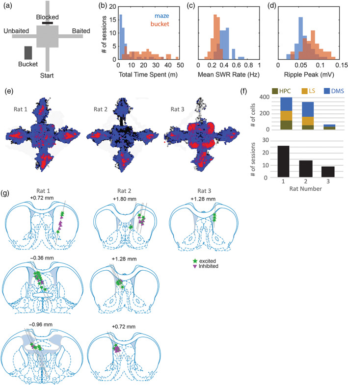
Behavioral and neurophysiological data samples. (a) Maze apparatus and holding bucket. (b) Total time spent sitting still on the maze versus in the bucket during each of 53 recording sessions. (c) Mean SWR rates during stillness on the maze versus in the bucket for each recording session. (d) Peak ripple amplitude during stillness on the maze versus in the bucket for each recording session. (e) Cumulative spatial distributions across recording sessions of all locations visited (black), locations where the rat sat still (blue), and locations where SWR events occurred (red) for each animal. (f) Number of cells recorded in each brain area (top graph) and total number of recording sessions (bottom) for each of the three rats in the study. (g) Septal and striatal recording sites for each rat; symbols indicate recording sites for cells that were excited (stars) versus inhibited (triangles) by SWR events

Over 6–8 days of initial training, rats learned to find food on one arm of the T‐maze. During this initial training period, hippocampal tetrodes were advanced until robust SWRs and theta rhythm were detected on two different tetrodes in the same hemisphere (see Section 4). These two tetrodes were assigned as the ripple and theta recording electrodes, respectively, and neither was advanced further during the remainder experiment. Starting with the next session, the goal and/or start arm was changed each time the rat achieved a criterion of 7/8 correct responses (see Section 4). Rats spent a median of 3.7 m on the maze and 19.9 m in the bucket during each session (Figure 1b). In the bucket and on the maze, SWR events were only measured during periods of stillness when the rat's running speed remained <2 cm/s for 3 s or more (Figure 1e). During these periods of stillness, the mean rate of SWR generation was significantly higher (paired t ₄₈ = 7.97, p = 2.4 × 10⁻¹⁰) on the maze (0.43 Hz) than in the bucket (0.28 Hz; Figure 1c), whereas the mean peak amplitude of SWR events was significantly higher (paired t ₄₈ = 16.7, p = 1.2 × 10⁻²¹) in the bucket (84 mV) than on the maze (63 mV; Figure 1d).

2.1. Cell sample

As summarized in Figure 1f, single units were recorded from the hippocampal CA1 region (n = 216 units from three rats), LS (n = 226 units from two rats), and DMS (n = 366 units from three rats). Hippocampal units were only analyzed in the hemisphere contralateral from the SWR detection site, to prevent confounds in the analysis that might arise from anatomical proximity between the SWR detection and single‐unit recording sites. Hence, single units in all three brain regions (CA1, LS, and DMS) were recorded several millimeters from the SWR detection site. To maximize the number of unique cells recorded throughout the experiment, tetrodes in LS and DMS were advanced by 333 μm after each behavior session, so that different units would be recorded in every session. By contrast, hippocampal tetrodes were advanced by at most 83 μm/day (and usually not at all), so that these tetrodes would remain within the hippocampal region throughout the entire experiment. Consequently, most hippocampal units were recorded more than once over multiple sessions, whereas LS and DMS units were recorded only once (during a single session) before the tetrode was advanced to find new cells. Analyses below include data only from the first session during which a given hippocampal unit was recorded, so that in all three structures (hippocampus, LS, and DMS), single‐unit responses were consistently analyzed using a single session's worth of data from each cell.

Figure 2 shows example data from Rat 1, obtained from a rat in which SWR events were recorded in the right hemisphere of CA1, while hippocampal units were recorded contralaterally in the left hemisphere of CA1 (Figure 2a). Example recordings are also shown for units recorded in left LS (Figure 2b) and right DMS (Figure 2c). Histology indicated that most septal units were recorded in LS, but a few were recorded the septofimbrial region (Figure 1g). Most striatal units were recorded in DMS, and only units localized to DMS (n = 366) were included in analyses presented below. Hippocampal unit data came from in or near the CA1 pyramidal layer (Figure 2a). Single‐unit responses to SWR events were measured only during periods of stillness (running speed <2 cm/s) in the bucket (Figure 2d1–f1) and on the maze (Figure 2d2–f2), whereas coherence of spike trains with hippocampal theta rhythm (Figure 2d3–f3) was measured during periods of active behavior on the maze (running speed >10 cm/s). We adopt the convention that the valley and peak of theta rhythm occur at phases 0° and 180°, respectively.

FIGURE 2.

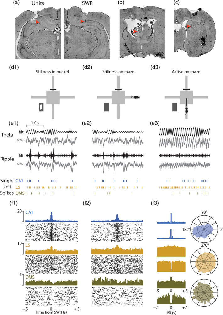
Example data from a single recording session. (a) Red arrows indicate example unit recording site in the left CA1 (left panel) and SWR detection site in right CA1 (right panel). (b) Example unit recording site in left septum. (c) Example unit recording site in right striatum. (d) Schematic diagrams for three different behavior conditions: Stillness in bucket (D1), stillness on maze (D2), and running on maze (D3). (e) Traces show 3 s of raw and filtered LFP data from theta (top row) and ripple (middle row) channels, aligned with examples of single unit spike rasters (bottom row) from a CA1, LS, and DMS; sample data is shown for stillness in bucket (E1), stillness on maze (E2), and running on maze (E3). (f) Example cell PETHs and rastergrams aligned to SWR events that occurred in the bucket (F1) or on the maze (F2). Two different interspike interval (ISI) autocorrelograms (F3, left) are shown for spikes recorded on the maze: One from −0.5 to +5 s with 2 ms bins (top graph in each row) to illustrate theta rhythmicity, and the other from −0.1 to +0.1 s with 1 ms bins (bottom graph in each row) to illustrate spike refractory periods. Polar plots (F3, right) show distributions of each example cell's spike phase relative to hippocampal theta

2.2. SWR‐evoked responses

To test how neurons responded to SWR events, a signed rank test was performed to compare each neuron's SWR‐evoked spike count in a 100 ms region of interest (ROI) spanning ±50 ms from each SWR peak, versus its baseline spike count before and after each corresponding SWR event (see Section 4). A Wilcoxon signed rank test was performed on baseline versus ROI spike counts for each cell, and the resulting p‐value was then converted to a log₁₀ scale to yield a negative number, which was flipped to positive if the ROI firing rate was greater than baseline (and retained as negative otherwise). This yielded a Sharp Wave Response Index (SWRI) for each cell, which was positive for cells that were excited by SWRs, and negative for cells that were inhibited by SWRs. Cells with SWRI > 2 were excited by SWRs with p < .01, and cells with SWRI < −2 were inhibited by SWRs with p < .01 (Figure 3a–c). Each cell's mean firing rate was calculated from speed‐filtered spikes that occurred during periods on the maze and in the bucket when running speed <2 cm/s, the same speed threshold used for SWR detection (see above). This was done so that subsequent analyses could examine how a neuron's SWR responsiveness was related to its mean firing rate during behavioral states similar to those when SWRs were recorded (see below).

FIGURE 3.

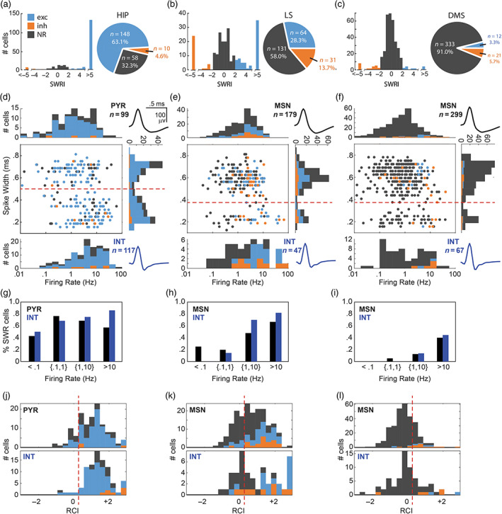
Unit responses to SWR events. Top row: Pie charts show proportions of neurons that were excited (exc), inhibited (inh), or nonresponsive (NR) to SWR events, while bar graphs show distributions of SWRI values in hippocampus (a), LS (b), and DMS (c). Second row: Scatter plots show spike width (y‐axis) versus mean firing rate (x‐axis) with accompanying bar graphs showing distributions of spike width (vertical), principal cell firing rates (horizontal above scatter plot), and interneuron firing rates (horizontal below scatter plot) for neurons in hippocampus (d), LS (e), and DMS (f). Third row: Bar graphs show percentage of SWR responsive cells (excited and inhibited combined) in four firing rate ranges (<0.1 Hz, 0.1–1.0 Hz, 1.0–10 Hz, and >10 Hz) for neurons recorded in hippocampus (g), LS (h), and DMS (i). Bottom row: Bar graphs show Rayleigh coherence index distributions for principal cells (top) and interneurons (bottom) recorded in hippocampus (j), LS (k), and DMS (l)

2.2.1. CA1

As explained above, CA1 neurons were analyzed only in the hemisphere contralateral from SWR detection. Excitatory responses to SWR events were observed in 148/216 (68.5%) of CA1 neurons (Figure 3a), which is consistent with prior reports showing that a large proportion of CA1 units fire during SWRs (Davidson et al., 2009; Foster & Wilson, ²⁰⁰⁶; Kudrimoti et al., ¹⁹⁹⁹; Skaggs & McNaughton, ¹⁹⁹⁶; Wilson & McNaughton, ¹⁹⁹⁴). By contrast, only 10/216 (4.7%) hippocampal neurons were inhibited during SWR events, but at least one SWR‐inhibited neuron was observed in the hippocampus of each rat. The remaining 58/216 (26.9%) of CA1 neurons were not significantly responsive during SWR events. A 3 × 3 chi‐square test indicated that similar proportions of CA1 cells were excited, inhibited, and nonresponsive during SWRs in all three rats, χ ² (4, n = 216) = 2.9, p = .57. Hippocampal neurons that were excited during SWRs usually exhibited their peak spike response within ±5 ms of the SWR onset, with a mean response latency of +4.3 ± 1.4 ms (SWR latency was measured from the time of peak ripple amplitude; see Section 4). The average latency for inhibitory SWR responses was slightly longer (+10.0 ± 7.1 ms), but did not differ significantly from the latency of excitatory responses (t ₁₄₅ = 1.04, p = .3; note the statistical power of this comparison was limited by the small sample of SWR‐inhibited neurons).

Single‐unit waveforms of hippocampal pyramidal cells versus interneurons can be discriminated with reasonable accuracy based on their spike widths and firing rates. Here, we found that CA1 spike widths (measured on the tetrode channel with the largest spike amplitude) were bimodally distributed, so that 99/216 (45.8%) units with spike widths >500 μs were classifiable as putative pyramidal cells, and 117/216 (54.2%) units with spike widths <500 μs were classifiable as putative interneurons (Figure 3d). The proportion CA1 units classified as pyramidal cells versus interneurons was similar in all three rats, χ ² (2, n = 216) = 1.7, p = .44, and a Mann–Whitney U test showed that putative interneurons had significantly higher firing rates than putative pyramidal cells (p = 5.3 × 10⁻⁷), as expected.

A 3 × 2 Chi‐square test indicated that SWR responsiveness (excited, inhibited, not responsive) was not contingent upon cell type (pyramidal vs. interneuron), χ ² (2, n = 216) = 2.6, p = .27. Hence, SWR‐evoked responses in CA1 were similarly prevalent among pyramidal cells and interneurons. Mann–Whitney U tests indicated that firing rates did not differ significantly for SWR responsive versus nonresponsive pyramidal cells (p = .79) or interneurons (p = .93), nor did they differ significantly for SWR‐excited versus inhibited pyramidal cells (p = .70) or interneurons (p = .90). Moreover, there was no significant correlation between log₁₀ firing rates (which were approximately normally distributed) and the absolute value of the SWRI for pyramidal cells (r = .01, p = .93) or interneurons (r = −.02, p = .6).

To further assess whether a neuron's SWR responsiveness depended upon its mean firing rate, we subdivided neurons into four firing rate tiers: very low (<0.1 Hz), low (0.1–1 Hz), medium (1–10 Hz), and high (>10 Hz). SWR‐responsive neurons in CA1 were observed at similar proportions in all four firing rate tiers (Figure 3g); only in the highest tier (where interneurons vastly outnumbered pyramidal cells) did interneurons appear to exhibit a higher proportion of SWR responsiveness than pyramidal cells, but there were so few pyramidal cells in this tier that it was not possible to make reliable comparisons. In summary, a large proportion of CA1 neurons were excited during SWRs, regardless of their cell type (pyramidal vs. interneuron) or mean firing rate.

2.2.2. LS

LS neurons were recorded from two of the three rats in the study (n = 121 units from Rat 1, n = 105 units from Rat 2). A majority of LS neurons (131/226, or 57.9%) were nonresponsive during SWRs, but 64/226 (28.3%) of LS neurons were excited and 31/226 (13.7%) were inhibited during SWR events (Figure 3b). The mean latency for excitatory SWR responses in LS was −4.6 ± 3.1 ms, and for inhibitory SWR responses was +10.0 ± 5.1 ms. Even though SWR‐excited LS neurons had negative mean response latency, this does not mean that LS neurons fired prior to the initiation of hippocampal sharp waves. SWR events are thought to originate in the CA3 subregion (Buzsáki, 2015; Csicsvari et al., ²⁰⁰⁰; Nakashiba et al., ²⁰⁰⁹), from which they are relayed to both CA1 and LS. A small negative response latency in LS implies that SWR events originating in CA3 can be detected a few milliseconds earlier by downstream unit spikes in LS than by the peak of the downstream LFP ripple in CA1. Since ripples are traveling waves (Patel et al., 2013), the measured latency between LS units responses and CA1 ripples should also depend partly upon the location at which SWRs are recorded in CA1, an issue that will be addressed further below.

As in CA1, spike widths were bimodally distributed in LS, suggesting the presence of at least two physiologically distinct types of LS neurons. Much like the striatum, LS contains GABAergic medium spiny projection neurons (MSNs) interspersed with various types of interneurons (Alonso & Frotscher, 1989; Leranth & Frotscher, ¹⁹⁸⁹). In single‐unit recordings, striatal MSNs tend to exhibit larger spike widths than interneurons (Yamin et al., 2013), and in our dataset, LS spike widths were bimodally distributed in such a way that 179/226 (79.2%) units with spike widths >350 μs were classifiable as putative MSNs, and 47/216 (20.8%) units with spike widths <350 μs were classifiable as putative interneurons (Figure 3e). A higher proportion of interneurons were recorded from Rat 1 (33%) than Rat 2 (6.7%), χ ² (1, n = 226) = 23.8, p < .00001, possibly because LS recording sites were more posteriorly located in Rat 1 than Rat 2 (Figure 1g). A Mann–Whitney U test found no significant difference between the firing rates of MSNs versus interneurons (p = .11).

A 3 × 2 Chi‐square test revealed that similar proportions of SWR‐evoked responses (excited, inhibited, and nonresponsive) were observed for MSNs versus interneurons,χ ² (2, n = 226) = 3.2, p = .2. When interneurons were omitted, firing rates of SWR‐responsive MSNs (excited and inhibited combined) were significantly higher than those of nonresponsive MSNs (p = 3.6 × 10⁻⁵). This result was independently replicated when the analysis was restricted only to MSN data from Rat 1 (p = .0015) or Rat 2 (p = .0024). When MSNs were omitted, firing rates of SWR responsive interneurons (excited and inhibited combined) were significantly higher than those of nonresponsive interneurons (p = 5.9 × 10⁻⁶). Consistent with this pattern, there was a significant negative correlation between log₁₀ firing rates and the absolute value of the SWR Responsive Index for both MSNs (r = −.25, p = 5.7e − 4) and interneurons (r = −.58, p = 1.6e − 5). When LS neurons were subdivided into firing rate tiers, only a small proportion (<20%) of SWR responsive neurons were observed in the lower firing rate tiers (<1 Hz), whereas larger proportions of SWR responsive neurons were observed in higher firing rate tiers (>1 Hz; Figure 3h). However, Mann–Whitney U tests found that mean firing rates did not differ for SWR‐excited versus inhibited MSNs (p = .79) or interneurons (p = .63). This pattern of results indicates that LS neurons with higher firing rates were more likely to be SWR responsive (excited or inhibited) than neurons with lower firing rates, and this was similarly true for both MSNs and interneurons.

2.2.3. DMS

DMS neurons were recorded from all three rats in the study. A majority (333/366, or 91%) of DMS neurons were found to be nonresponsive to SWRs (Figure 3c). Only 12/366 (3.3%) of DMS neurons were excited during SWR events (but at least two SWR‐excited neurons were observed in each of the three rats), whereas 21/366 (5.7%) of DMS neurons were inhibited during SWR events (with roughly similar percentages in all three rats: Rat 1: 4.5%, Rat 2: 7.7%, Rat 3: 0%). The mean latency for excitatory SWR responses in DMS was +36.8 ± 10.8 ms, and for inhibitory responses in striatum was +15.0 ± 8.4 ms.

DMS spike widths were bimodally distributed in such a way that cells could be separated into subpopulations of putative MSNs versus interneurons. Accordingly, 299/366 (81.6%) units with spike widths >350 μs were classified as putative MSNs, and 67/366 (18.3%) units with spike widths <350 μs were classified as putative interneurons (Figure 3f). A Mann–Whitney U test found no significant difference between firing rates of MSNs versus interneurons (p = .12). The proportion of interneurons observed in DMS was quite similar for Rat 1 (29%; 45/155) and Rat 3 (32%; 9/28), but considerably fewer interneurons were recorded in Rat 2 (7%; 13/183), possibly because the DMS recording site for Rat 2 was more posterior than in Rats 1 or 3 (Figure 1g). When data from all three rats was pooled together, a 3 × 2 Chi‐square test indicated that similar proportions of SWR‐evoked responses (excited, inhibited, and not responsive) were observed for each cell type (MSN vs. interneuron), χ ² (2, n = 366) = .47, p = .79. There was significant negative correlation between the log₁₀ firing rates and absolute values of the SWRI for MSNs (r = −.27, p = 2.7e − 6). Consistent with this, firing rates of SWR‐responsive MSNs (excited and inhibited combined) were significantly higher than those of nonresponsive MSNs (p = 4.6 × 10⁻⁶). For interneurons, there was also a significant negative correlation between the log₁₀ firing rates and absolute value of the SWRI (r = −.37, p = .002), and again, firing rates of SWR‐responsive interneurons were higher than those of nonresponsive interneurons (p = .0013). When DMS neurons were subdivided into firing rate tiers, almost all of the SWR responsive neurons were found to be in the highest firing rate tier (Figure 3i). However, firing rates did not differ significantly for SWR‐excited versus inhibited MSNs (p = .58) or interneurons (p = .57) in DMS. In summary, this pattern of results indicates that only DMS neurons with the highest firing rates were SWR responsive (excited or inhibited), and this was similarly true for putative MSNs and interneurons.

2.3. Coherence with hippocampal theta rhythm

To quantify the coherence of a neuron's spike train with hippocampal theta rhythm, we measured the phase of theta rhythm at which individual spikes occurred, and then plotted a circular distribution of phases over all spikes generated by the neuron during active movement on the maze (running speed >10 cm/s). A Rayleigh Coherence Index (RCI) was computed from the p‐value of a Rayleigh test for circular nonuniformity performed on each individual cell's spike phase distribution (see Section 4). RCI values were approximately normally distributed (Figure 3j–l), making it possible to perform parametric statistical comparisons of theta coherence between different cell populations. Any cell with RCI > 0.3 had a significantly nonuniform theta phase distribution (see Section 4) and was classified as a “theta coherent” cell.

It is important to note that RCI does not measure how strongly a cell's spike train is modulated by theta rhythm, but instead measures the tendency to fire at a specific phase of the hippocampal LFP. That is, the RCI quantifies periodicity in the cross‐correlation between the spike train and the theta LFP, not periodicity in the auto‐correlation of the spike train with itself, and it is possible to have one without the other (Zeitler et al., 2006). Some neurons that exhibited strong spike coherence with hippocampal theta rhythm (and thus large RCI values) also exhibited strong theta rhythmicity of their own spike trains (e.g., see the SWR‐excited DMS interneuron from Rat #1 in upper right of Figure 4c), while other neurons with large RCI values exhibited little or no theta rhythmicity in their own spike trains, despite being phase locked to the hippocampal LFP (e.g., the SWR‐inhibited LS interneurons from Rat #1 in right panels of Figure 4b). The preferred firing phase of each theta coherent cell was measured as the circular mean of its phase distribution (see below).

FIGURE 4.

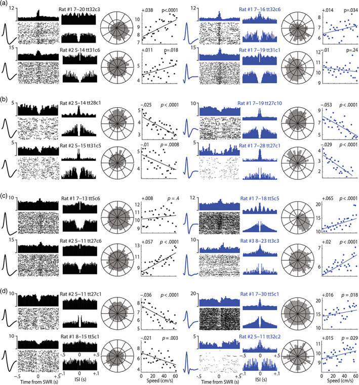
Example cells recorded in LS and DMS. Waveforms and histograms for MSNs are shown in black, and for interneurons in blue. The spike rastergram and peristimulus time histogram shown for each cell was triggered by the first 200 SWR events that occurred during a session (maze and bucket combined). Two ISI autocorrelograms are shown for each cell, one from −0.5 to +0.5 s (top) and the other from −0.1 to +0.1 s (bottom). A circular distribution of spike phases relative to theta rhythm in the hippocampal LFP is shown for each cell. Scatterplots show each cell's mean firing rate (y‐axis) at a given running speed (x‐axis), with regression line showing linear fit to the scatter points; slope of speed modulation (in Hz/cm/s) and p‐value of Pearson correlation are shown at upper left and right, respectively, of each scatterplot. (a) LS neurons excited by SWRs. (b) LS neurons inhibited by SWRs. (c) DMS neurons excited by SWRs. (d) DNS neurons inhibited by SWRs

A three‐way independent ANOVA revealed that mean RCI values were different for neurons recorded in CA1, LS, and DMS (F _2,784 = 1961, p = 4.2e − 70). Post hoc comparisons revealed that mean RCI values were greater in CA1 than LS (t ₄₄₀ = 4.7, p = 2.5e − 6) or DMS (t ₅₇₉ = 19.6, p = 6.2e − 66), and greater in LS than DMS (t ₅₈₉ = 13.4, p = 4.3e − 36). Consistent with this result, a 3 × 2 Chi‐square test revealed that the proportion of theta coherent cells was highly contingent upon brain region, χ ² (1, n = 799) = 237.6, p < .00001; 87.5% (189/216) of CA1 neurons were classified as theta coherent, compared with 65.5% (148/226) of LS neurons and only 23.2% (85/366) of DMS neurons. In summary, CA1 neurons were more theta coherent than LS neurons, which in turn were more theta coherent than DMS neurons.

2.3.1. CA1

CA1 pyramidal cells and interneurons both exhibited robust coherence of their spike trains with theta rhythm (Figure 3j). RCIs were significantly higher for interneurons than pyramidal cells (t ₂₁₄ = 3.1, p = .0024), and consistent with this result, the proportion of interneurons classified as theta coherent (94.5%; 86/91) was significantly higher than the proportion of pyramidal cells (82.4%, 103/125), χ ² (1, n = 216) = 7.1, p < .0079. In all three individual rats, a greater proportion of interneurons than pyramidal cells were theta coherent: Rat 1, 96.6% (56/58) of interneurons versus 88.6% (62/70) of pyramidal cells, Rat 2, 88.2% (15/17) of interneurons versus 84.4% (27/32) of pyramidal cells, Rat 3, 93.8% (15/16) of interneurons versus 60.9% (14/23) of pyramidal cells. These results are in agreement with established findings that hippocampal interneurons—commonly referred to as “theta cells”—are often strongly phase locked to theta rhythm during locomotion.

Theta coherence and SWR responsiveness

Among putative pyramidal cells, a three‐way independent ANOVA revealed that RCIs differed for cells that were excited, inhibited, or nonresponsive during SWR events (F _2,122 = 8.5, p = .0003). Post hoc comparisons indicated that SWR‐excited pyramidal cells were significantly more theta coherent than nonresponsive pyramidal cells (t ₁₂₀ = 4.2, p = 6.2e − 5). Accordingly, a significantly higher proportion of SWR‐excited (88.9%, 73/81) than nonresponsive (65.6%, 27/41) pyramidal cells were theta coherent, χ ² (1, n = 122) = 9.4, p = .002. RCI values of SWR‐inhibited pyramidal cells did not differ significantly from nonresponsive pyramidal cells (t ₄₂ = 1.1, p = .29), but only three SWR‐inhibited pyramidal cells were recorded (all from Rat 1, and all classified as theta‐coherent), so the sample size was not large enough to meaningfully compare theta coherence between SWR responsive versus nonresponsive pyramidal cells. RCI values did not differ for SWR‐inhibited versus SWR‐excited pyramidal cells (t ₈₂ = .11, p = .92).

Among putative interneurons, RCIs also differed for cells that were excited, inhibited, or nonresponsive during SWR events (F _2,88 = 8.3, p = .0005). Post hoc comparisons revealed that, in contrast with pyramidal cells, RCI values of SWR‐excited interneurons were not different from those of nonresponsive interneurons (t ₈₂ = 1.0, p = .32), whereas SWR‐inhibited interneurons were significantly more theta coherent than both SWR‐excited interneurons (t ₇₂ = 4.0, p = 1.5e − 4) and nonresponsive interneurons (t ₂₂ = 3.2, p = .0038). The sample size of SWR‐inhibited interneurons was small (n = 7), but all were theta coherent, and at least one SWR‐inhibited interneuron was recorded in each rat.

In summary, CA1 pyramidal cells and interneurons were both significantly more likely to be theta coherent if they were responsive to SWRs (either excited or inhibited) than if they were nonresponsive to SWRs. It should be emphasized that theta coherence was measured during locomotion, whereas SWR responsiveness was measured during stillness, so these two variables were measured during mutually exclusive behavioral states. It thus appears that CA1 neurons that are strongly phase‐locked to the hippocampal LFP during locomotion in the theta state also tend to be strongly phase locked to the LFP during the quiescence in the SWR state.

Preferred firing phases

Rayleigh tests were performed on distributions of preferred firing phases from SWR‐excited CA1 neurons that were theta coherent (Figure 5a, top row). Preferred phases were found to be nonuniformly distributed in each of the three individual rats (Rat 1: Z ₈₀ = 6.3, p = .0017; Rat 2: Z ₂₈ = 16.6, p = 2.8e −9; Rat 3: Z ₂₈ = 5.2, p = .0047). The population mean of preferred phases differed somewhat in each rat (Rat 1: 188.2°, Rat 2: 224.0° and Rat 3: 221.9°), but was within 45° of the theta peak at 180° in all three rats. The phase of the theta LFP is graded along the septotemporal axis of CA1 (Lubenov & Siapas, 2009; Patel et al., ²⁰¹²), and as noted above, LFPs were recorded in the hemisphere contralateral from CA1 units. Hence, variability in the mean phase of SWR‐excited cells across rats may have arisen from rat‐specific differences in the mean septotemporal offset between LFP and single‐unit recording sites. To compensate for these differences among rats, the preferred phase of each unit was shifted by adding an angle equal to ϕ _r  − 180°, where ϕ _r denotes the mean phase at which the population of SWR‐excited hippocampal neurons fired in rat r. After shifting single‐unit phases from different rats into this common reference frame, phase data was pooled across rats for analysis (“All Rats” column in Figure 5a). Note that if a unit's ϕ‐shifted phase is 180°, then it fires in phase with the mean for SWR‐excited CA1 units recorded in the same rat. Conversely, if the unit's ϕ‐shifted phase is 0°, then it fires in antiphase with the mean for SWR‐excited CA1 units in the same rat.

FIGURE 5.

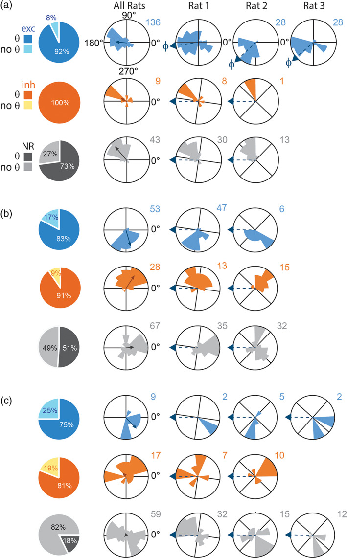
Preferred theta phase and SWR responsiveness. Each row shows data for neurons that were excited (exc), inhibited (inh), or nonresponsive (NR) to SWR events in CA1 (a), LS (b), or DMS (c). Pie charts show proportion of each cell type that spiked coherently (θ) or noncoherently (no θ) with theta rhythm. Leftmost column of polar plots shows circular distributions of preferred firing phases for θ‐coherent cells pooled across all rats. Right columns show polar plots of preferred firing phases in individual rats. In the top row, arrows at rims of polar plots show mean theta phase, ϕ _r , of SWR‐excited hippocampal cells from rat r. Phase data from individual rats was rotated by ϕ _r prior to being pooled in the leftmost polar plot column (see main text)

After pooling across rats, the distribution of ϕ‐shifted phases for theta coherent CA1 neurons that were nonresponsive to SWRs (Figure 5a, bottom row) passed the Rayleigh test (Z ₄₃ = 23.9, p = 5.8e − 13); their mean firing phase was 147.0°, which was significantly different from the 180° mean ϕ‐shifted phase of SWR‐excited CA1 cells (Watson‐Williams test, F _1,178 = 18.3, p = 3.0e − 5). Hence, theta coherent cells that did not respond to SWRs fired an average of 33° earlier in the theta cycle than those that were excited during SWRs. Of the SWR nonresponsive neurons that were theta coherent, 62.8% (27/43) were classified as pyramidal cells and 37.2% (16/43) as interneurons. Pyramidal cells passed the Rayleigh test (Z ₂₇ = 17.5, p = 5.4e − 10) with a mean phase of 145.2°, and interneurons passed the Rayleigh test (Z ₁₆ = 6.7, p = 6.9e − 4) with a mean phase of 150.8°. A Watson–Williams test found no significant difference between the firing phases of nonresponsive pyramidal cells versus interneurons (F _1,42 = .14, p = .71). Hence, firing phases were similar for pyramidal cells and interneurons that did not respond to SWRs.

The distribution of ϕ‐shifted phases for theta coherent CA1 neurons that were inhibited during SWRs (Figure 5a, middle row) did not pass the Rayleigh test (Z ₁₀ = .95, p = .3944), but this test lacked power because the sample size was small (n = 10). Of these SWR‐inhibited neurons, 30% (3/10) were classified as pyramidal cells and 70% (7/10) as interneurons, and neither subpopulation passed the Rayleigh test on its own. A larger sample of SWR‐inhibited cells would be needed to accurately estimate the distribution of their preferred firing phases.

2.3.2. LS

MSNs and interneurons in LS both exhibited coherence of their spike trains with theta rhythm: 66.5% (119/179) of MSNs and 61.7% (29/47) of interneurons were classified as theta coherent (Figure 3k). Mean RCI values were higher for interneurons than MSNs (t ₂₂₄ = 2.1, p = .034), but the proportion of theta coherent cells was not significantly different for MSNs versus interneurons, χ ² (1, n = 226) = .38, p = .54. Hence, while a similar proportion of MSNs and interneurons in LS were theta coherent, the strength of coherence was greater for interneurons than MSNs. Mean firing rates during stillness did not differ for theta coherent versus noncoherent MSNs (t ₁₇₇ = 1.38, p = .17) or interneurons (t ₄₅ = .45, p = .65).

Theta coherence and SWR responsiveness

Among putative MSNs, a three‐way independent ANOVA revealed that RCIs differed for cells that were excited, inhibited, or nonresponsive during SWR events (F _2,176 = 20.6, p = 9.2e − 9). Post hoc comparisons indicated that SWR‐excited MSNs were significantly more theta coherent than nonresponsive MSNs (t ₁₅₅ = 5.0, p = 1.4e − 6). Accordingly, a significantly higher proportion of SWR‐excited (81.3%, 39/48) than nonresponsive (54.1%, 59/109) MSNs were theta coherent, χ ² (1, n = 157) = 10.5, p = .0012. Theta coherence remained more prevalent among SWR‐excited than nonresponsive MSNs when the analysis was repeated on data from individual rats: Rat 1, 85.3% (29/34) of excited versus 78.1% (32/41) of nonresponsive cells, Rat 2, 85.7% (12/14) of excited versus 36.8% (25/68) of nonresponsive cells. RCI values of SWR‐inhibited MSNs were also significantly larger than nonresponsive MSNs (t ₁₂₉ = 5.1, p = 1.3e − 6). Accordingly, a significantly higher proportion of SWR‐inhibited (95.5%, 21/22) than nonresponsive (54.1%, 59/109) MSNs were theta coherent, χ ² (1, n = 131) = 10.5, p = .0003. Theta coherence remained more prevalent among SWR‐inhibited than nonresponsive MSNs when analysis was restricted to data from individual rats: Rat 1, 100% (6/6) of inhibited versus 78.1% (32/41) of nonresponsive cells, Rat 2, 87.5% (12/14) of inhibited versus 36.8% (25/68) of nonresponsive cells. RCI values of SWR‐inhibited MSNs did not differ from those of SWR‐excited MSNs (t ₄₂ = 1.1, p = .29).

Among putative interneurons, RCIs also differed for cells that were excited, inhibited, or nonresponsive during SWR events (F _2,44 = 14.6, p = 3.0e − 6). Similar to MSNs, post hoc comparisons indicated that SWR‐excited interneurons were significantly more theta coherent than nonresponsive interneurons (t ₃₆ = 6.0, p = 6.6e − 7). Accordingly, a significantly higher proportion of SWR‐excited (87.5%, 14/16) than nonresponsive (36.4%, 8/22) interneurons were theta coherent, ${\chi }^2$ (1, n = 38) = 9.9, p = .0017. Theta coherence was more prevalent among SWR‐excited than nonresponsive interneurons in individual rats: Rat 1, 71.4% (10/14) of excited versus 41.2% (7/17) of nonresponsive cells, Rat 2, 100% (2/2) of excited versus 60% (3/5) of nonresponsive cells. RCI values of SWR‐inhibited interneurons were also significantly larger than those of nonresponsive interneurons (t ₂₉ = 3.5, p = .0017). It should be noted that all of the SWR‐inhibited interneurons (n = 9) were recorded from Rat 1 (none were recorded from Rat 2), and of these, 88.9% (8/9) were theta coherent. SWR‐excited versus inhibited interneurons did not differ significantly from one another in theta coherence (t ₂₃ = 1.4, p = .18).

Preferred firing phases

To achieve consistent phase referencing across rats and brain regions, firing phases of LS units were shifted by the rat's mean phase of SWR‐excited CA1 neurons (ϕ _r ) prior to pooling across rats (see Section 2.3.1.2). The distribution of pooled firing phases for all SWR‐excited LS neurons that were theta coherent (Figure 5b, top row) passed the Rayleigh test (Z ₅₃ = 23.6, p = 2.6e − 12) with a mean firing phase of 292.1°. Of these LS neurons, 73.6% (39/53) were classified as MSNs and 26.4% (14/53) as interneurons. MSN phases passed the Rayleigh test (Z ₃₉ = 22.1, p = 4.6e − 12) with a mean phase of 296.0°. Interneurons had a similar mean phase of 273.6°, and also passed the Rayleigh test (Z ₁₄ = 2.9, p = .0506). A Watson–Williams test found no significant difference between the mean firing phases of SWR‐excited MSNs versus interneurons (F _1,52 = 1.42, p = .24). Circular V‐tests found that the mean firing phase for SWR‐excited theta coherent cells (MSNs and interneurons combined) was indistinguishable from the center of the downslope of theta cycle at 270° (V ₅₃ = 35.1, p = 4.8e − 12), but distinct from the 180° peak of theta (V ₅₃ = 4.3, p = .1991), and from the 0° valley of theta (V ₅₃ = ‐4.3, p = .8009). Hence, theta coherent LS neurons that were excited during SWRs showed a significant preference for firing near the center of the downslope of the theta cycle.

The distribution of pooled phases for SWR‐inhibited LS neurons that were theta coherent (Figure 5b, middle row) also passed the Rayleigh test (Z ₂₈ = 11.5, p = 3.0e − 6), with a mean firing phase of 85.1°. Of these neurons, 75% (21/28) were classified as MSNs and 25% (7/28) as interneurons. MSN phases passed the Rayleigh test (Z ₂₁ = 9.9, p = 1.5e − 5) with a mean phase of 66.9°, and interneuron phases also passed (Z ₇ = 5.5, p = .0014) with mean phase of 131.6°. A Watson–Williams test revealed that mean firing phases differed significantly for SWR‐inhibited MSNs versus interneurons (F _1,27 = 10.9, p = .0028). However, while the mean phases of MSNs versus interneurons were distinguishable from one another, circular V‐tests indicated that mean firing phases of MSNs (V ₂₁ = 13.2, p = 2.2e − 5) and interneurons (V ₇ = 4.6, p = .0066) were not distinguishable from the center of the upslope of the theta cycle at 90°. Taken together, these results suggest that in LS, SWR‐inhibited cells that were theta coherent preferred to fire nearly in antiphase with SWR‐excited cells, by spiking near the center of the upslope of the theta cycle, although MSNs fired a bit earlier and interneurons fired a bit later than the center of the upslope.

The distribution of pooled phases for LS neurons that were nonresponsive to SWRs (Figure 5b, bottom row) also passed the Rayleigh test (Z ₆₇ = 8.4, p = 1.8e − 4), with a mean firing phase of 372.2°. Of these neurons, 88.1% (59/67) were classified as MSNs and 11.9% (8/67) as interneurons. MSNs passed the Rayleigh test (Z ₅₉ = 8.1, p = 2.4e − 4) with a mean phase of 19.3° that was not distinguishable from the valley of hippocampal theta at 0° (V ₅₉ = 20.7, p = 7.1e − 5), but was distinguishable from the center of the upslope (V ₅₉ = 7.2, p = .0917) and of the downslope (V ₅₉ = −7.2, p = .9083). Interneurons did not pass the Rayleigh test (Z ₁₄ = 2.6, p = .0731), suggesting that their preferred phases were not unimodal. These results suggest that in LS, theta coherent MSNs that did not respond to SWRs tended to fire near the valley of hippocampal theta.

2.3.3. DMS

The striatum receives considerably less input from the hippocampus than LS, and accordingly, putative MSNs and interneurons exhibited less theta coherence in DMS than in LS: 21.7% (65/299) of MSNs and 29.9% (20/67) of interneurons were classified as theta coherent in DMS (Figure 3l). Mean RCI values trended higher for interneurons than MSNs in DMS (t ₃₆₄ = 1.8, p = .071). An independent t‐test compared log₁₀ firing rates during stillness for DMS neurons that were classified as theta coherent versus those that were not. This analysis included all MSNs recorded in DMS, regardless of whether they were excited, inhibited, or nonresponsive during SWR events. Firing rates did not differ for theta coherent versus noncoherent MSNs (t ₂₉₆ = .33, p = .74) or interneurons (t ₆₅ = .26, p = .8), indicating that across the entire populations of DMS neurons, theta coherence was similarly prevalent across the range of observed firing rates.

Theta coherence and SWR responsiveness

Among MSNs, a three‐way independent ANOVA revealed that RCIs differed for cells that were excited, inhibited, or nonresponsive during SWR events (F _2,297 = 33.8, p = 6.0e − 14). Post hoc comparisons indicated that SWR‐excited MSNs had significantly larger RCIs than nonresponsive MSNs (t ₂₈₀ = 4.0, p = 8.7e − 5). Accordingly, across all three rats, a significantly larger proportion of SWR‐excited (70.0%, 7/10) than nonresponsive (16.5%, 45/272) MSNs were classified as theta coherent, ${\chi }^2$ (1, n = 282) = 18.3, p = 1.9e − 5. The total sample size of SWR‐excited DMS cells was small (n = 10), but at least one such cell was observed in each rat, and the proportion of theta‐coherent cells was higher for SWR‐excited than nonresponsive MSNs in all three rats: Rat 1, 50% (1/2) of excited versus 17.1% (18/105) of nonresponsive cells, Rat 2, 71.4% (5/7) of excited versus 18.8% (28/149) of nonresponsive cells, Rat 3, 100% (1/1) of excited versus 22.2% (4/18) of nonresponsive cells. RCIs of SWR‐inhibited MSNs were also significantly larger than those of nonresponsive MSNs (t ₂₈₆ = 7.5, p = 1.1e − 12). SWR‐inhibited MSNs were only recorded from Rat 1 and Rat 2, and in both rats, a greater proportion of theta‐coherent SWR‐inhibited than nonresponsive MSNs was observed: Rat 1, 100% (3/3) of inhibited versus 17.1% (18/105) of nonresponsive cells, Rat 2, 76.9% (10/13) of inhibited versus 18.8% (28/149) of nonresponsive cells. RCI values of SWR‐excited versus inhibited MSNs did not differ significantly (t ₂₄ = 1.3, p = .22).

Among interneurons, a three‐way independent ANOVA revealed that RCIs differed for cells that were excited, inhibited, or nonresponsive during SWR events (F _2,64 = 10.1, p = .0002). Post hoc comparisons indicated that SWR‐excited interneurons had significantly larger RCIs than nonresponsive interneurons (t ₆₀ = 4.1, p = 1.4e − 4). Only two SWR‐excited DMS interneurons were recorded (one from Rat 1, the other from Rat 3), but both (100%) were theta coherent, which was a higher proportion than the 23.3% (14/60) of nonresponsive interneurons were classified as theta coherent (binomial test, p = .0529). RCIs of SWR‐inhibited interneurons were also significantly larger than those of nonresponsive interneurons (t ₆₃ = 2.6, p = .0131). Accordingly, a significantly larger proportion of SWR‐inhibited (80.0%, 4/5) than nonresponsive (23.3%, 14/60) interneurons were classified as theta coherent, ${\chi }^2$ (1, n = 65) = 7.4, p = .0065. SWR‐inhibited DMS interneurons were recorded from two of the three rats, and were significantly more likely to be theta coherent than nonresponsive interneurons in both rats: Rat 1, 75% (3/4) of inhibited versus 12.5% (5/40) of nonresponsive cells, Rat 2, 100% (1/1) of inhibited versus 16.7% (2/12) of nonresponsive cells. RCI values of SWR‐excited versus inhibited interneurons did not differ significantly (t ₅ = 1.15, p = .3).

Preferred firing phases

To achieve consistent phase referencing across rats and brain regions, firing phases of DMS units were shifted by the rat's mean phase of SWR‐excited CA1 neurons (ϕ _r ) prior to pooling across rats (see Section 2.3.1.2). The distribution of pooled phases for SWR‐excited DMS neurons that were theta coherent (Figure 5c, top row) passed the Rayleigh test (Z ₁₂ = 6.8, p = 4.7e − 4), with a mean firing phase of 316.8°. Of these neurons, 58.3% (7/12) were classified as MSNs and 41.7% (5/12) as interneurons. MSN phases passed the Rayleigh test on their own (Z ₇ = 3.2, p = .0356) with a mean firing phase of 314.0°, and while interneurons had a similar mean firing phase of 322.4°, they did not pass the Rayleigh test (Z ₅ = 1.3, p = .31), possibly owing to their small sample size. Taken together, these results suggest that SWR‐excited neurons in DMS that were theta coherent preferred to fire just prior to the valley of hippocampal theta.

The phase distribution for SWR‐inhibited DMS neurons that were theta coherent (Figure 5c, middle row) did not pass the Rayleigh test (Z ₂₀ = 1.3, p = .28). Of these neurons, 65% (13/20) were classified as MSNs and 35% (7/20) as interneurons. Neither of these two subpopulations had phase distributions that passed the Rayleigh test (MSNs: Z ₁₃ = .68, p = .52; interneurons: Z ₇ = 1.2, p = .31). Hence, we found no evidence for a consistent phase preference among SWR‐inhibited neurons in DMS that were theta coherent.

The phase distribution for theta coherent neurons that were nonresponsive to SWRs (Figure 5c, bottom row) also did not pass the Rayleigh test (Z ₆₈ = .83, p = .43). Of these neurons, 79.4% (54/68) were classified as MSNs and 21.6% (14/68) as interneurons. MSN phases did not pass the Rayleigh test (MSNs: Z ₅₄ = .52, p = .6), so there was no evidence for a consistent phase preference among SWR‐inhibited MSNs in DMS that were theta coherent. However, a Rayleigh test on interneuron phase preferences yielded a trend toward nonuniformity (Z ₁₄ = 2.6, p = .0731), with a mean phase preference of 167.2°. Hence, some theta coherent DMS interneurons that do not respond during SWRs may fire near the peak of the theta cycle, approximately in antiphase with SWR‐excited MSNs in DMS that are theta coherent.

2.4. Running speed sensitivity

To analyze modulation of neural firing rates by running speed, we performed a linear regression analysis upon plots of firing rate versus running speed for each recorded cell (see Section 4). Neurons were only included in the speed analysis if their firing rates were sampled across a sufficiently wide range of running speeds (see Section 4). The slope of the regression line (in units of Hz/cm/s) was taken as a measure of the sign and depth of speed modulation. Cells with positive speed modulation slopes exhibited a positive correlation of their firing rates with running speed, and shall henceforth be referred to as positive speed (S+) cells. Cells with negative speed modulation slopes had firing rates that were negatively correlated with running speed, and shall henceforth be referred to as negative speed (S−) cells.

2.4.1. CA1

Of all recorded CA1 neurons, 39.8% (86/216) met criteria for inclusion in analysis of speed modulation, and of these, 66/86 (76.7%) exhibited a significant linear correlation (p < .05) of their firing rates with running speed (Figure 6a). Half of these speed‐modulated CA1 neurons were pyramidal cells (33/66), and the other half was interneurons (33/66). A large majority (95.5%, 63/66) of speed‐modulated CA1 cells were S+ cells, whereas only 4.5% (3/65) of speed‐modulated CA1 cells (one pyramidal cell and two interneurons) were S‐ cells. Among CA1 cells that met criteria for speed analysis, 75.4%, (43/57) of the SWR‐responsive (either excited or inhibited) cells were speed modulated, whereas 79.3% (23/29) of SWR nonresponsive cells were speed modulated. Hence, modulation by running speed was not contingent upon SWR responsiveness, ${\chi }^2$ (1, n = 86) = .16, p = .69. In summary, ~75% of CA1 cells that were eligible for speed analysis were S+ cells (regardless of whether they were pyramidal cells or interneurons, and regardless of whether they responded to SWRs), and less than 5% were S− cells.

FIGURE 6.

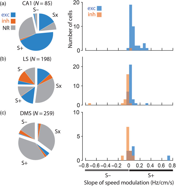
Speed modulation and SWR responsiveness. Pie charts show proportions of all neurons in each brain region that were eligible for speed analysis that were positively (S+), negatively (S−), or not significantly (Sx) modulated by running speed. Within each speed classification, shading of wedges indicates proportions of cells that were excited (exc), inhibited (inh), or nonresponsive (NR) to SWR events. Histograms show the distribution of speed slopes for SWR‐excited (blue) and SWR‐inhibited (orange) cells that were significantly modulated by running speed. (a) CA1; (b) LS; (c) DMS

2.4.2. LS

Of the 226 neurons recorded in LS, 198 (87.6%) met criterion for inclusion in the analysis of speed modulation, and of these 94/198 (47.5%) exhibited a significant linear correlation (p < .05) of their firing rates with running speed. About 80% (158/198) of these speed‐modulated LS neurons were MSNs, and the remaining 20% (40/198) were interneurons, which was similar to the overall proportion of MSNs and interneurons in the entire LS population. About half of eligible MSNs (46.2%, 73/158) and half of eligible interneurons (52.5%, 21/40) were significantly modulated by running speed; hence, modulation by running speed was not contingent upon cell type, ${\chi }^2$ (1, n = 198) = .51, p = .48. Of the LS neurons that were speed modulated, 45/95 (47.4%) were S+ cells and 49/95 (52%) were S− cells (Figure 6b, left). Hence, speed‐modulated neurons in LS were split nearly in half between S+ and S− cells, and this was true of both MSNs (45% positively modulated, 55% negatively modulated) and interneurons (57% positively modulated, 43% negatively modulated). It was also true of both individual rats (Rat #1: 25 S+ and 25 S− cells; Rat #2: 20 S+ and 24 S− cells).

A significantly larger proportion of SWR responsive LS neurons (58.5%, 55/94 neurons that were excited or inhibited during SWRs) than nonresponsive neurons (34.6%, 36/104) were modulated by running speed, ${\chi }^2$ (1, n = 198) = 11.4, p = .0008. A large majority (96.3%, 26/27) of SWR‐responsive S+ cells in LS were excited (rather than inhibited) by SWRs, and 88.4% (23/26) of these were also theta coherent. Conversely, a majority (75%, 21/28) of SWR‐responsive S− cell in LS were inhibited by SWRs, and 90.5% (19/21) of these were also theta coherent. A Chi‐square test indicated that among SWR‐responsive LS neurons that were speed modulated, the sign of the SWR response was highly contingent upon the sign of speed modulation, ${\chi }^2$ (1, n = 55) = 29.1, p < .00001. That is, LS cells that were excited by SWRs tended to also be S+ cells, and LS cells that were inhibited by SWRs tended to also be S− cells. This was further confirmed by the observation that among speed‐modulated LS cells that were excited during SWRs, the mean slope of speed modulation was significantly greater than zero (0.028 ± 0.011 Hz/cm/s; signed rank test, p = .006), whereas the mean slope of speed modulation for SWR‐inhibited cells was significantly less than zero (mean −0.06 ± 0.033 Hz/cm/s; signed rank test, p = .0002). A Wilcoxon rank‐sum test confirmed that among speed‐modulated LS neurons, slopes for SWR‐excited cells were significantly different from SWR‐inhibited cells (p = 4.6e − 6). To test whether this result depended upon two outlying slopes with large values (Figure 6b, right), a t‐test was run after removing these outliers (the slope distributions became normal when outliers were removed, permitting the use of parametric statistics). The slope distributions differed significantly even when outliers were removed from the analysis (t ₅₁ = 5.18, p = 3.8e − 6).

These results indicate that among LS neurons that were both SWR responsive and speed modulated, S+ cells were usually excited by SWRs, whereas S− cells were usually inhibited by SWRs. A possible confound for this analysis could be that, because SWRs were only recorded during stillness, statistical power to detect inhibition during SWRs might be greater for S− cells, and statistical power to detect excitation during SWRs might be greater for S+ cells. This concern arises because S− cells are defined as those that fire at a higher rate during stillness than movement, so it may be easier to detect SWR‐induced inhibition of S− cells against their higher background firing rates during stillness. Conversely, S+ cells are defined as those that fire at a higher rate during movement than stillness, so it may be easier to detect SWR‐induced excitation against their lower background firing rates during stillness. However, the median firing rate during stillness (estimated here by the y‐intercept of the speed slope fit line) did not differ (rank sum test Z = 0.682, p = .5) for SWR‐responsive S+ cells (median 4.4 Hz) versus S− cells (median 3.8 Hz), nor did it differ (rank sum test Z = 1.33, p = .18) for speed modulated cells that were excited (median 4.6 Hz) versus inhibited (median 3.3 Hz) during SWRs. Hence, variation in background firing rates during stillness is not likely to explain the strong contingency we observed between the sign of SWR responsiveness and the sign of the speed modulation slope.

This contingency between the signs of SWR responses and speed slopes remained significant when the analysis was restricted only to MSNs, or only to interneurons. Among SWR‐responsive MSNs that were classified as S+ cells, 94.4% (17/18) were excited by SWRs and only one was inhibited; among SWR‐responsive MSNs that were classified as S− cells, 74.4% (15/21) were inhibited by SWRs and 25.6% (6/21) were excited, ${\chi }^2$ (1, n = 39) = 17.4, p3.1e − 5. Among SWR‐responsive interneurons that were classified as S+ cells, 100% (9/9) were excited by SWRs and none were inhibited; among SWR‐responsive MSNs that were classified as S− cells, 85.7% (6/7) were inhibited by SWRs and only one was excited. Chi‐square analysis on interneurons was not possible, because zero S+ interneurons were inhibited by SWRs. However, given that 62.5% (10/16) of all speed‐modulated LS interneurons were excited by SWRs, and 37.5% (6/16) were inhibited, binomial tests indicated that it was significant to observe nine SWR‐excited neurons out of nine S+ cells (p = .0145), and six SWR‐inhibited neurons out of seven S− cells (p = .0132).

The contingency between the signs of SWR responses and speed slopes also remained significant when the analysis was restricted only data from Rat 1 or Rat 2. Among SWR‐responsive S+ neurons from Rat 2, 87.5% (6/7) were excited by SWRs and only one was inhibited; among SWR‐responsive S− neurons from Rat 2, 91.7% (11/12) were inhibited by SWRs and 8.3% (1/12) were excited, ${\chi }^2$ (1, n = 19) = 11.4, p = 7.4e − 4. Among SWR‐responsive S+ neurons from Rat 1, 100% (20/20) were excited by SWRs and none were inhibited; among SWR‐responsive S− neurons from Rat 1, 62.5% (10/16) were inhibited by SWRs and 37.5% (6/16) were excited. Chi‐square analysis of neurons from Rat 1 was not possible because zero S+ cells were inhibited by SWRs. However, given that 72.2% (26/36) of all speed‐modulated LS neurons from Rat 1 were excited by SWRs, and 27.8% (10/36) were inhibited, binomial tests indicated that it was significant to observe 20 SWR‐excited neurons out of 20 S+ cells (p = .0014), and 6 SWR‐inhibited neurons out of 7 S− cells (p = .0039).

In summary, we found LS neurons that responded to SWRs were more likely to be speed modulated than cells that did not respond to SWRs. Wirtshafter and Wilson (2019) conversely reported no relationship between SWR responsiveness and speed modulation of LS neurons, but in that study, only excitatory (and not inhibitory) responses of LS neurons were considered. To compare our current data against these prior finings, we replicated the prior study's approach by re‐classifying SWR‐inhibited LS cells as nonresponsive; after doing this, only 35.8% (34/94) of SWR‐excited LS neurons were modulated by running speed, which does not differ significantly from the 45.6% (57/125) of nonresponsive neurons (now including SWR‐inhibited neurons) that were modulated by running speed, ${\chi }^2$ (1, n = 198) = .018, p = .89. Hence, if only excitatory responses to SWRs are considered, as in Wirtshafter and Wilson (2019), then we replicate their finding of no relationship between SWR responsiveness and speed modulation in LS. Note that most speed‐modulated LS neurons that were excited during SWRs were S+ cells, and most speed‐modulated LS neurons that were inhibited during SWRs were S− cells. This result has potentially important implications for the role of the hippocampal–LS pathway in motivated behavior (see Section 3).

2.4.3. DMS

Of the 366 neurons recorded in DMS, 247 (67.5%) met criterion for inclusion in the analysis of speed modulation. We found that 156/247 (63.2%) of these neurons exhibited a significant linear correlation (p < .05) of their firing rates with running speed. About 80% (158/198) of these speed‐modulated LS neurons were MSNs, and the remaining 20% (40/198) were interneurons, which was similar to the overall proportion of MSNs and interneurons in the entire LS population.

Two thirds of eligible MSNs (66.7%, 136/204) and about half of eligible interneurons (46.5%, 20/43) in DMS were found to be modulated by running speed; based on these proportions, a significantly larger percentage of MSNs than interneurons were modulated by running speed, ${\chi }^2$ (1, n = 247) = 6.2, p = .0128. Of all DMS neurons that were speed modulated, 110/156 (70.5%) were positively and 46/156 (29.5%) were negatively correlated with running speed (Figure 6c, left). Hence, DMS neurons were more likely to be positively than negatively modulated by running speed, and this was true of both MSNs (72.8% positively modulated, 27.2% negatively modulated) and interneurons (55% positively modulated, 45% negatively modulated). The proportion of positively versus negatively modulated cells did not differ significantly for MSNs versus interneurons, ${\chi }^2$ (1, n = 156) = 2.7, p = .1032, but did differ across rats, ${\chi }^2$ (2, n = 156) = 15.4, p = 4.5e − 4 (Rat #1: 25 positive and 25 negative speed cells; Rat #2: 66 positive and 18 negative speed cells; Rat #2: 19 positive and 3 negative speed cells). Similar proportions of SWR responsive DMS neurons (70.4%, 19/27 neurons excited or inhibited during SWRs) and nonresponsive neurons (62.3%, 137/220) were modulated by running speed, ${\chi }^2$ (1, n = 247) = .68, p = .4104.

A majority (66.7%, 6/9) of SWR‐responsive DMS cells with significant positive speed modulation slopes were excited by SWRs, and 100% (6/6) of these cells were theta coherent. A majority (80%, 8/10) of SWR‐responsive DMS cells with significant negative speed modulation slopes were inhibited by SWRs, and 75% (6/8) were theta coherent. A Chi‐square test on these proportions indicated that among SWR‐responsive DMS neurons that were speed modulated, the sign of the SWR response was contingent upon the sign of speed modulation, ${\chi }^2$ (1, n = 19) = 4.2, p = .0397. Hence, DMS cells that were excited by SWRs tended to be positively modulated by running speed, and DMS cells that were inhibited by SWRs tended to be negatively modulated by running speed. Accordingly, for speed‐modulated cells that were excited during SWRs, the mean slope of speed modulation was greater than zero (0.112 ± 0.088 Hz/cm/s), but not by a significant margin (signed rank test, p = .0781), whereas the mean slope for SWR‐inhibited cells was less than zero (−0.017 ± 0.013 Hz/cm/s), but also not by a significant margin (signed rank test, p = .1748). A Wilcoxon rank‐sum test found that among speed‐modulated DMS neurons, slopes for SWR‐excited cells differed significantly from SWR‐inhibited cells (p = .0203). Hence, even though slopes of speed modulation did not differ significantly from zero for SWR‐excited or inhibited cells (probably because the tests were underpowered by small sample sizes), they did differ significantly from one another, supporting the conclusion that their slopes were of opposing sign.

In summary, DMS neurons that responded to SWRs were just as likely to be speed modulated as cells that did not respond to SWRs, in contrast with LS, where speed modulation was more prevalent among SWR‐responsive neurons (see above). Positively sloped speed cells were more prevalent than negatively sloped speed cells in DMS, in contrast with LS, where positive and negative slopes were observed in equal proportions. Most speed‐modulated DMS neurons that were excited during SWRs had positive speed slopes, and most speed‐modulated DMS neurons that were inhibited during SWRs had negative speed slopes, similar to what was observed in LS. However, there was a rather small sample of DMS neurons with significant SWR responsiveness and significant speed modulation (n = 19), and for this reason, it was not possible to further subdivide the sample to test whether the contingency between the signs of SWR responses and speed slopes remained significant when the analysis was restricted only to specific types of neurons (MSNs vs. interneurons), or to data from individual rats.

2.5. Responses to reward

To analyze neural responses to reward delivery, we computed peristimulus histograms triggered by the rat's arrivals at the end of whichever maze arm had been chosen on a given trial (see Section 4). Two histograms were computed for each cell: one triggered by rewarded arrivals, and the other by unrewarded arrivals (Figure 7). A neuron was classified as reward responsive if rewarded versus nonrewarded trials differed significantly (p < .01 for Mann–Whiney U) in their postarrival but not prearrival firing rates. In all three brain structures, a proportion of neurons were classified as R+ cells that responded more during rewarded than nonrewarded arrivals: 16.2% (35/216) in CA1, 10.6% (24/226) in LS, and 9.3% (34/366) in DMS. A similar proportion of neurons in each region were classified as R− cells that responded more during nonrewarded than rewarded arrivals: 8.8% (19/216) in CA1, 11.5% (26/226) in LS, and 8.2% (30/366) in DMS. A 3 × 3 Chi‐square test found no contingency between reward responsiveness (R+, R−, nonresponse to reward) and brain region (CA1, LS, and DMS), ${\chi }^2$ (4, n = 808) = 8.6, p = .07. Hence, similar distributions of reward responsive neurons were observed in all three structures.

FIGURE 7.

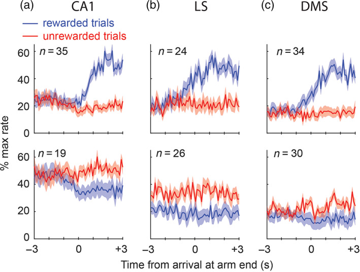
Reward responses. Top and bottom rows of graphs show population‐averaged responses of R+ and R− cells, respectively, in CA1 (a), LS (b), and DMS (c). All significantly responsive cells are included in the population average, regardless of SWR responsiveness. Responses are plotted as a percentage of each cell's peak firing rate in the response window, and shading indicates standard error for each 100 ms time bin

2.5.1. CA1

A 3 × 2 Chi‐square test found no contingency between sharp wave responsiveness (excited, inhibited, or nonresponsive to SWR) and reward responsiveness (responsive vs. nonresponsive) of CA1 neurons, ${\chi }^2$ (2, n = 216) = .85, p = .65. Hence, there was no clear relationship between the responsiveness of CA1 neurons to SWRs and their responsiveness to reward. Of the 35 CA1 neurons classified as R+ cells, 18 (51%) were pyramidal cells and 17 (49%) were interneurons. Of the 19 CA1 neurons classified as R− cells, 4 (21%) were pyramidal cells and 15 (79%) were interneurons. Of the 162 CA1 neurons that did not respond to reward, 77 (48%) were pyramidal cells and 85 (52%) were interneurons. A 3 × 2 Chi‐square test found a trend toward contingency between reward responsiveness (R+, R−, nonresponse to reward) and cell type (pyramidal vs. interneuron) in CA1, ${\chi }^2$ (2, n = 216) = 5.3, p = .07, mainly driven by the fact that R− cells were more likely to be interneurons than pyramidal cells. The population averaged response for R− cells in CA1 (Figure 7a) shows that these cells were mostly inhibited during trials when reward was encountered (rather than excited during trials when no reward was encountered), and had a higher normalized baseline (prearrival) firing rate than R+ cells. Hence, R− cells in CA1 tended to be interneurons with high firing rates that were inhibited during encounters with reward. By contrast, R+ cells were equally like to be pyramidal cells or interneurons, and robustly increased their firing rates when reward was encountered.

2.5.2. LS

A 3 × 2 Chi‐square test found no contingency between sharp wave responsiveness and reward responsiveness of LS neurons, ${\chi }^2$ (2, n = 226) = 1.02, p = .6. Hence, in LS, there was no clear relationship between responsiveness to SWRs and responsiveness to reward. By contrast, Wirtshafter and Wilson (2019) reported that in LS, SWR responsive neurons were more likely to be modulated by reward than SWR nonresponsive neurons. But as noted above (see Section 2.3.2), in that study, only excitatory (and not inhibitory) responses of LS neurons were measured. To test whether this discrepancy might account for our failure to replicate a relationship between SWR responsiveness and reward responsiveness in LS, we repeated the analysis with SWR‐inhibited cells reclassified as SWR nonresponsive. However, a 2 × 2 Chi‐square test again indicated that there was no contingency between SWR responsiveness (excited vs. nonexcited) and reward responsiveness, ${\chi }^2$ (1, n = 226) = .17, p = .68.

Of the 24 LS neurons classified as R+ cells, 16 (67%) were MSNs and 8 (33%) were interneurons. Of the 26 LS neurons classified as R− cells, 24 (92%) were MSNs and 2 (8%) were interneurons. Of the 176 LS neurons that did not respond to reward, 139 (79%) were MSNs and 37 (21%) were interneurons. A 3 × 2 Chi‐square test found a trend toward contingency between reward responsiveness and cell type in LS, ${\chi }^2$ (2, n = 226) = 4.9, p = .08, mainly driven by the fact that R− cells were more likely to be interneurons than MSNs. Some R− cells in LS were inhibited during trials when reward was encountered, whereas others were excited during trials when no reward was encountered; these two effects cancel out in the population averaged response for R− neurons, which is why pre‐ and postarrival firing rates look similar for rewarded and nonrewarded trials (Figure 7b). R+ cells robustly increased their firing rates when reward was encountered, and the proportion of MSNs versus interneurons among R+ cells was similar to that for all neurons recorded in LS.

2.5.3. DMS

A 3 × 2 Chi‐square test found no contingency between sharp wave responsiveness and reward responsiveness of DMS neurons, ${\chi }^2$ (2, n = 366) = .62, p = .73. Hence, in DMS, there was no clear relationship between responsiveness to SWRs and responsiveness to reward. Of the 34 DMS neurons classified as R+ cells, 20 (59%) were MSNs and 14 (41%) were interneurons. Of the 30 DMS neurons classified as R− cells, 26 (87%) were MSNs and 4 (13%) were interneurons. Of the 302 DMS neurons that did not respond to reward, 253 (84%) were MSNs and 49 (16%) were interneurons. A 3 × 2 Chi‐square test found a significant contingency between reward responsiveness and cell type in DMS, ${\chi }^2$ (2, n = 226) = 13.3, p = .0013, mainly driven by the fact that R− cells were more likely to be interneurons than MSNs. R− cells in DMS tended to have low firing rates; some R− cells were inhibited during trials when reward was encountered, whereas others were excited during trials when no reward was encountered, and these two effects partly cancel out in the population averaged response for R− neurons (Figure 7c). In summary, R− cells in DMS were mostly MSNs, whereas R+ cells were more evenly divided between MSNs and interneurons. R+ cells robustly increased their firing rates when reward was encountered, and the proportion of MSNs versus interneurons among R+ cells was similar to that for all neurons recorded in DMS.

3. DISCUSSION

A growing body of evidence suggests that hippocampal projections to LS may be an important route via which the hippocampus relays information to the midbrain and striatum to exert influence over behaviors such as reward‐seeking, motor actions, reinforcement learning, and decision making (Bender et al., 2015; Gomperts et al., ²⁰¹⁵; Luo et al., ²⁰¹¹; McGlinchey & Aston‐Jones, ²⁰¹⁸; Tingley & Buzsáki, ²⁰¹⁸; Wirtshafter & Wilson, ²⁰¹⁹). Prior studies have demonstrated that septal neurons can encode an animal's position in their firing rates (Takamura et al., 2006) as well as their spike phases (Tingley & Buzsáki, 2018). Septal projections to the midbrain may thus relay information from the hippocampus to dopaminergic and hypothalamic circuits that attach motivational value to locations and states, and then on to striatal circuits that rely upon hippocampal information for model‐based reinforcement learning and decision making processes (Mattar & Daw, 2018; Stachenfeld et al., ²⁰¹⁷; van der Meer & Redish, ²⁰¹⁰).

3.1. Hippocampal processing states

The theta and SWR states of the hippocampal EEG are likely to play important roles in regulating the flow of information from hippocampus through LS to the midbrain and striatum. To interpret the findings we have reported here, and discuss their potential significance, it is helpful to review some background on what is known about these two distinct processing states.

3.1.1. Theta state

During the theta state, as an animal locomotes through its environment, hippocampal place cells fire selectively at preferred spatial locations (O'Keefe & Dostrovsky, 1973). Place cells have long been hypothesized to encode cognitive maps of familiar spatial environments (O'Keefe & Nadel, ¹⁹⁷⁸; Redish, ¹⁹⁹⁹), and may also encode predictive representations of future states that aid in decision making (Mattar & Daw, 2018; Stachenfeld et al., ²⁰¹⁷). As an animal passes through a place cell's preferred firing location (or place field), place cells burst rhythmically at a slightly higher frequency than the LFP theta frequency, causing spikes to exhibit phase precession against the LFP (O'Keefe & Recce, ¹⁹⁹³). At the population level, phase precession segregates place cell spikes in time so that cells with place fields that lie ahead of the animal's current location fire at late phases of LFP theta, whereas cells with place fields behind the animal's current location fire early phases of LFP theta (Dragoi & Buzsáki, 2006; Skaggs & McNaughton, ¹⁹⁹⁶; Wikenheiser & Redish, ²⁰¹⁵). Similar phase coding of spatial locations has been shown to occur in LS (Monaco et al., 2019; Tingley & Buzsáki, ²⁰¹⁸). Recent evidence suggests that the downslope of the theta cycle may be dominated by forward sequences of hippocampal place cell activity that extend ahead of the animal toward the direction in which it is traveling, whereas the upslope of the theta cycle may be dominated by reverse sequences that extend behind the animal, backward toward the direction it is coming from (Kay et al., 2020; Wang et al., ²⁰²⁰). Here, we observed that LS contains S+ and S− cells that fire during the downslope and upslope of hippocampal theta, respectively. We shall propose below (Section 3.2.2) that these LS neurons may play a role in selecting motor actions based upon predictions that are generated during forward and reverse theta sequences, and thereby aid in decisions about whether to change course or continue navigating along the current trajectory.

3.1.2. SWR state

When an animal is at rest, the hippocampal LFP switches from the theta state to the LIA state, during which SWRs are accompanied by brief population bursts of place cell activity, referred to as compressed replay events, that can be decoded as “imagined” spatial trajectories through an environment (Davidson et al., 2009; Diba & Buzsáki, ²⁰⁰⁷; Foster & Wilson, ²⁰⁰⁶; Karlsson & Frank, ²⁰⁰⁹; Lee & Wilson, ²⁰⁰²; Skaggs & McNaughton, ¹⁹⁹⁶). While an animal is running on a maze, replay events occur during pauses in motor activity and tend to encode trajectories that start or end at the animal's current location (Diba & Buzsáki, 2007; Jackson et al., ²⁰⁰⁶; Johnson & Redish, ²⁰⁰⁷; Karlsson & Frank, ²⁰⁰⁹; Pfeiffer & Foster, ²⁰¹³; Wu et al., ²⁰¹⁷). While an animal is resting in a different environment after a maze session, replay events may encode trajectories from various start and end points within a recently experienced maze environment (Buzsák, 1998; Wilson & McNaughton, ¹⁹⁹⁴).

Compressed replay events that occur during SWRs have been hypothesized to play three distinct but related roles in reinforcement learning. First, it has been proposed that during navigation, forward replay of alternative future trajectories supports deliberation over the best future path for the animal to take from its current location (Johnson & Redish, 2007; Mattar & Daw, ²⁰¹⁸; Pfeiffer & Foster, ²⁰¹³; Wu et al., ²⁰¹⁷; Yu & Frank, ²⁰¹⁵). Second, it has been proposed that when reward outcomes are obtained, compressed replay of prior trajectories that have been traversed in the recent past may help to solve the “credit assignment” problem in reinforcement learning, which is the problem of assigning credit or blame for outcomes to decisions that were made in the remote past, before the outcome was obtained (Ambrose et al., 2016; Foster & Wilson, ²⁰⁰⁶; Singer & Frank, ²⁰⁰⁹). Third, it has been proposed that during sleep, compressed replay during SWRs may be necessary for consolidating short‐term memories of recent experiences to long‐term storage (Buzsák, 1998; Ego‐Stengel & Wilson, ²⁰¹⁰; Girardeau & Zugaro, ²⁰¹¹; Wilson & McNaughton, ¹⁹⁹⁴). The septal output pathway from the hippocampus could play an important role in all three of these hypothesized functions for SWR events. Supporting this, SWR‐evoked responses have been shown to occur in subpopulations of septal neurons (Tingley & Buzsáki, 2020), including septal neurons that respond to rewards (Wirtshafter & Wilson, 2019). Reward‐responsive midbrain dopamine neurons tend to fire synchronously with SWRs during wakeful stillness on a maze (but not during sleep), as might be expected if the animal were assessing the values of potential action plans during SWRs that occur on the maze (Gomperts et al., 2015).

3.2. Hippocampal modulation of LS neurons

Evidence suggests that SWR events typically originate in the CA3 region of the hippocampus, from which they are monosynaptically transmitted to CA1 via Schaffer collaterals (Buzsáki, 2015; Csicsvari et al., ²⁰⁰⁰; Nakashiba et al., ²⁰⁰⁹). Consequently, a large proportion of hippocampal CA1 neurons are excited during SWRs, as reported here and in prior studies (Davidson et al., 2009; Foster & Wilson, ²⁰⁰⁶; Kudrimoti et al., ¹⁹⁹⁹; Skaggs & McNaughton, ¹⁹⁹⁶; Wilson & McNaughton, ¹⁹⁹⁴). CA1 and CA3 both send monosynaptic projections to LS (Risold & Swanson, 1997), so it is not surprising that LS contains neurons that respond during SWRs, as reported here and elsewhere (Tingley & Buzsáki, 2020; Wirtshafter & Wilson, ²⁰¹⁹).

3.2.1. S+ and S− neurons in LS

Wirtshafter and Wilson (2019) reported that SWR‐responsive LS neurons were more likely than nonresponsive neurons to fire coherently with hippocampal theta rhythm during periods of locomotion, and that the firing rates of some SWR‐responsive LS neurons were positively or negatively modulated by the rat's running speed. Both of these prior results were replicated in the current study. But in contrast with Wirtshafter and Wilson's (2019) finding that SWR responsiveness was not related to speed modulation in the LS population, we found that SWR‐responsive LS neurons were more likely to be modulated by running speed than SWR nonresponsive neurons. This discrepancy may have arisen because Wirtshafter and Wilson (2019) only considered LS neurons that were excited during SWRs, and not those that were inhibited. Accordingly, when we classified only SWR‐excited (but not SWR‐inhibited) LS neurons as SWR responsive, we also found no relationship between SWR responsiveness and speed modulation. Only by considering inhibitory as well as excitatory responses of LS neurons to SWRs were we were able to observe that SWR‐responsive LS cells were more likely to be speed modulated than SWR nonresponsive LS cells. Moreover, we also observed an additional novel relationship: SWR‐excited LS neurons tended to show positively sloped modulation of their firing rates by running speed (and most were thus classified as S+ cells), whereas SWR‐inhibited LS neurons tended to show negatively sloped modulation of their firing rates by running speed (and most were thus classified as S− cells).

During the theta state, SWR‐excited S+ cells preferred to fire during the downslope of the theta cycle, whereas SWR‐inhibited S− cells tended to fire during the upslope of the theta cycle. A possible mechanistic explanation for the existence of these two opponent cell populations could be that S+ and S− cells reciprocally inhibit one another, as might be expected if S+ cells were GABAergic MSNs and S− cells were GABAergic interneurons (or vice versa) that reciprocally project onto one another. However, S+ and S− cells did not divide neatly along the boundary separating MSNs from interneurons. An alternative possibility is that LS contains distinct two distinct neural subcircuits that are engaged during behavioral activation (e.g., during high running speed) versus inhibition (e.g., during low running speed), and that each subcircuit is composed from its own distinct subpopulations of both MSNs and interneurons. For example, S+ cells might predominate among MSNs within the activation subcircuit and among interneurons within the inhibition subcircuit, while S− cells would conversely predominate among MSNs within the inhibition subcircuit and interneurons within the activation subcircuit (or vice‐versa). Such an arrangement would be consistent with our observations that S+ and S− cells were both found in similar proportions among MSNs as well as interneurons within LS.

Wirtshafter and Wilson (2019) reported that SWR‐responsive LS neurons were more likely than nonresponsive neurons to be modulated by rewards and reward predictive cues, and they interpreted this as evidence that reward responsive LS neurons were preferentially connected with the hippocampus. Here, we replicated the finding that a subset of LS neurons was modulated by reward (Figure 7), but in contrast with Wirtshafter and Wilson (2019), we found no relationship between the responsiveness of LS neurons to SWRs and rewards.

3.2.2. Go‐stop error signal hypothesis

As explained above, we found that the valence of an LS neuron's SWR response (excitation versus inhibition) predicted the sign of its speed sensitivity as well as its preferred firing phase during theta rhythm (Figure 5b). SWR‐excited S+ cells in LS fired most during the downslope of the theta cycle, whereas SWR‐inhibited S− cells in LS fired most during the upslope of the theta cycle. As noted above, prior studies (Dragoi & Buzsáki, 2006; Skaggs & McNaughton, ¹⁹⁹⁶; Wang et al., ²⁰²⁰; Wikenheiser & Redish, ²⁰¹⁵) have shown that phase precession causes place cells encoding locations ahead of the animal to fire on the downslope of theta (which should be concurrent with S+ cell spikes), whereas place cells encoding locations behind the animal fire on the upslope of theta (which should be concurrent with S− cell spikes).

Theta‐frequency alternation between hippocampal representations of forward versus rearward locations (Kay et al., 2020; Wang et al., ²⁰²⁰) could be mechanism for repeatedly generating temporal difference (TD) prediction error signals to compare the expected values of two mutually exclusive action plans: behavioral activation (continued running) versus inhibition (slowing or stopping). Such a prediction error signal would need to be computed repeatedly and frequently by a moving animal, since the relative values of these two action plans could change suddenly as a function of the animal's changing location in the environment. By definition, a TD error signal measures the time derivative of expected value, $V_t-V_{t-1}$, where $V_t$ is the value of a currently active representation and $V_{t-1}$ is the value of a previously active representation (Sutton & Barto, 1998). Hence, theta frequency alternation between representations of forward versus rearward locations could generate a “go‐stop” TD error signal that oscillates at the theta frequency between $V_F-V_R$ (the value of forward minus rearward locations) and $V_R-V_F$ (the value of rearward minus forward locations). A larger go–stop error signal on one phase of theta would indicate a greater value for running than stopping (and thereby activate running), whereas a larger go–stop error signal on the opposing phase of theta would indicate a greater value for stopping than running (and thereby inhibit running). Such a go–stop error signal could be computed from hippocampal outputs that are relayed to the midbrain via LS, since LS is known to project to midbrain targets containing neurons that generate prediction error signals (Montague et al., 1996; Schultz, ¹⁹⁹⁸). Consistent with this hypothesis, it has been shown that disruption of theta rhythm in the pathway from hippocampus to LS, or from LS to midbrain, disrupts behavioral regulation of running speed in freely behaving mice (Bender et al., 2015).

If opposing phases of the theta cycle are responsible for encoding the predicted outcomes of running versus stopping, then this might help to explain our present finding that LS contains two populations of neurons that fire on opposing phases of theta: S+ neurons that fired on the downslope of theta and were positively correlated with running speed, versus S− neurons that fired on the upslope of theta and were negatively correlated with running speed. We also observed that S+ neurons were excited during SWRs, whereas S− neurons were inhibited during SWRs. This makes sense under the assumption that SWRs are similar to “single‐shot downslopes” of the theta cycle. During the theta state, future trajectories can be subdivided into two major categories: those traversable by behavioral activation (continued running toward forward locations, represented on the theta downslope) versus those traversable by behavioral inhibition (discontinued running to backtrack toward rearward locations, represented on the theta upslope). But during the SWR state, when the animal is sitting still, behavioral activation is required to reach all locations except for the current location. The category of locations reachable by behavioral inhibition thus collapses onto the current location, and all other trajectories fall into the “behavioral activation” category, represented by the theta upslope during running. It might thus be expected that the activity of S+ and S− neurons during SWRs should be similar to their activity during the theta upslope (rather than downslope), as we observed here.

3.3. Hippocampal modulation of DMS neurons

Prior studies have shown that ventral striatal neurons exhibit phasic responses during hippocampal SWRs (Lansink et al., 2009; Sjulson et al., ²⁰¹⁸; Sosa et al., ²⁰²⁰). Here we observed SWR‐evoked responses in the dorsal striatum, specifically in DMS. However, <10% of recorded DMS neurons were excited or inhibited during SWRs.

3.3.1. SWR‐evoked responses in DMS

As in LS, DMS neurons showed a significant contingency between SWR responsiveness and theta coherence. Only about one fourth of DMS neurons were theta coherent, and <10% of DMS neurons were SWR responsive, but a majority (about 80%) of SWR‐responsive DMS neurons were also classified as theta coherent, suggesting that a subpopulation of hippocampally influenced DMS neurons are modulated by both hippocampal theta rhythm during locomotion and by SWRs during stillness. SWR‐evoked responses were similarly prevalent among MSNs and interneurons in DMS, so hippocampal signals did not appear to preferentially influence one cell type over the other. DMS neurons that were excited by SWRs tended to have firing rates that were positively modulated by running speed, whereas DMS neurons that were inhibited by SWRs tended to have firing rates that were negatively modulated by running speed, as we observed in LS. But in contrast with LS, these two DMS subpopulations did not clearly segregate their spikes to different phases of the hippocampal theta cycle. Our observation of speed‐modulated DMS neurons is consistent with previous single‐unit recording studies reporting that firing rates of striatal neurons in rodents are correlated with the animal's running speed (Rueda‐Orozco & Robbe, 2015).

It should be noted that SWR‐evoked responses were most prevalent among DMS neurons with high mean firing rates during stillness, whereas SWR‐evoked responses were almost nonexistent among DMS cells with low mean firing rates (Figure 3i). Indeed, about 40% of DMS neurons with firing rates >10 Hz were responsive to SWRs. One possible explanation for this could be that a high firing rate is necessary condition for achieving the statistical power needed to detect weak hippocampal influences upon DMS neurons. If so, then DMS neurons with lower firing rates might also be weakly influenced by hippocampal activity, but much longer recording times would be required to achieve the statistical power needed to detect such weak influences.

This statistical power issue is relevant not only for data analysis, but also for neural signaling within the brain itself. Neural firing rates tend to be log normally distributed within a population (Buzsáki & Mizuseki, 2014), such that low rate cells are exponentially more common than high rate cells by an order of magnitude that scales with the rate difference. One functional reason for this might be to skew the distribution of neural response sensitivities so that the majority of cells (those with low firing rates) are primarily sensitive to strong influences from primary input sources, whereas a minority of cells (those with high firing rates) are able to leverage their high spike counts to detect weaker influences from nonprimary input sources. If so, DMS neurons with high firing rates might function as “sensitive ears” for detecting the relatively weak influence of nonprimary input to DMS such as inputs from the hippocampus.

3.3.2. Action selection and habit learning

Projection cells from the striatum are GABAergic MSNs, which can be broadly subdivided into two main classes expressing D1 versus D2‐type dopamine receptors. Classical models of the basal ganglia posit that D1 MSNs are the origin of a “direct” striatonigral motor output pathway which excites motor behavior, whereas D2 MSNs are the origin of an “indirect” striatopallidal motor output pathway which inhibits motor behavior. However, neural recording and imaging studies have consistently failed to find evidence that D1 and D2 MSNs behave simply as motor‐on and motor‐off cells, as classical models would seem to predict. Instead, both types of MSNs seem to fire together during initiation and execution of voluntary motor behaviors (Cui et al., 2013; Isomura et al., ²⁰¹³). Combined with other evidence, these findings have led to speculation that D1 MSNs may help to drive the execution of selected actions, while D2 MSNs may simultaneously inhibit the execution of competing nonselected actions (Tecuapetla et al., 2016). We were unable to distinguish between D1 and D2 MSNs in the current study, and this might help to explain our failure to observe any consistent theta firing phase for SWR‐excited versus SWR‐inhibited DMS neurons. SWRs are hypothesized to provide a mechanism for animals to deliberate over which actions to select versus suppress (Kay et al., 2020; Mattar & Daw, ²⁰¹⁸; Yu & Frank, ²⁰¹⁵), which may be regarded as tantamount to sorting out which actions should be excited by the D1 population and which should be suppressed by the D2 population. It would thus be worthwhile in future studies to investigate whether excitatory versus inhibitory responses during SWRs are differentially distributed among D1 versus D2 subtypes of MSNs. It might be found that SWR‐excited D1 MSNs and SWR‐inhibited D2 MSNs are both positively correlated with running speed, and both fire together during the same phase of theta to promote continued running when forward locations have higher expected outcome value than rearward locations. On the opposing phase of theta, SWR‐excited D2 MSNs and SWR‐inhibited D1 MSNs (both negatively correlated with running speed) might fire together to promote cessation of running when rearward locations have higher expected outcome value than forward locations. Under such an arrangement, neither SWR‐excited nor SWR‐inhibited MSNs would fire consistently at the same phase of theta (as we observed), because D1 and D2 neurons would exhibit opposing relationships between the valence of their SWR response and the sign of their speed modulation slope. It should be noted that we recorded SWR events during stillness, when overt motor actions were not being performed. Hence, the SWR‐responsive striatal cells we observed might be MSNs that are involved in persistently inhibiting motor behavior, and thereby preventing actual motor actions from being performed during “virtual” navigation.

Another possible role for SWR‐evoked responses in DMS arises from prior evidence that acquisition of maze learning tasks is impaired by disruption of SWRs during both waking and sleeping states (Girardeau et al., 2009; Jadhav et al., ²⁰¹²). This has been interpreted as evidence that offline SWRs are involved in consolidation of episodic memories that are necessary for task performance. The cortex is commonly regarded as a primary storage target for such episodic memory consolidation (Frankland et al., 2001; Squire & Alvarez, ¹⁹⁹⁵), but some striatal regions may be targeted as well. Repeated performance of instrumental tasks (including maze navigation) is thought to induce a transition from model‐based (or goal‐directed) action selection during early repetitions of the task, to model‐free (or habit‐driven) action selection during later repetitions of the task (Mattar & Daw, 2018; Packard & McGaugh, ¹⁹⁹⁶). Evidence suggests that the hippocampus and prefrontal cortex interact with DMS to govern model‐based decision making, whereas the dorsolateral striatum is more involved in governing model‐free action selection (Balleine et al., 2007; Geerts et al., ²⁰²⁰; Thorn et al., ²⁰¹⁰; Yin & Knowlton, ²⁰⁰⁴). If hippocampus and DMS are partners in model‐based learning and decision making, then SWRs may be involved in consolidating associations between specific place representations activated during replay and specific patterns of action selection that are required to achieve correct performance in instrumental tasks. This possibility could be further investigated by future experiments in which striatal unit activity is selectively disrupted during SWRs.

3.4. Summary and conclusions

SWRs are frequently accompanied by compressed replay of spatial trajectories within hippocampal place cell populations (Davidson et al., 2009; Diba & Buzsáki, ²⁰⁰⁷; Foster & Wilson, ²⁰⁰⁶; Karlsson & Frank, ²⁰⁰⁹; Lee & Wilson, ²⁰⁰²; Skaggs & McNaughton, ¹⁹⁹⁶), and similar replay trajectories are generated during theta rhythm (Dragoi & Buzsáki, 2006; Kay et al., ²⁰²⁰; Skaggs & McNaughton, ¹⁹⁹⁶; Wang et al., ²⁰²⁰; Wikenheiser & Redish, ²⁰¹⁵). Findings presented here suggest that replay of spatial trajectories during SWR events and theta oscillations may be accompanied by activation of motor representations in LS and DMS which encode actions that would be necessary to follow replayed trajectories. Hence, when mental representations of a particular trajectory become active within hippocampal place cell populations—either during an SWR event or during a theta sequence driven by phase precession—a corresponding representation of the motor action necessary to follow that trajectory may be concurrently activated within LS and DMS. This concurrent activation of hippocampal state representations and subcortical action representations might support neural computations that are essential for reinforcement learning and value‐based decision making.

Reinforcement learning theory (Sutton & Barto, 1998) suggests that value‐based decision policies can be optimized by attaching values not just to representations of states (such as locations in an environment) or actions (such as performing a specific motor behavior), but also to state‐action pairs (such as performing a specific action at a specific location). SWRs might therefore support learning and decision making by activating representations of spatial trajectories and motor actions at the same time. For example, deliberation over alternative future trajectories during SWRs might not only involve activating hippocampal representations of spatial locations that lie along those trajectories (Johnson & Redish, 2007; Pfeiffer & Foster, ²⁰¹³; Yu & Frank, ²⁰¹⁵), but could additionally require activating representations of motor actions that must be performed at each location to successfully navigate along that trajectory. Similarly, when assigning credit or blame for outcomes of recent behavioral choices (Ambrose et al., 2016; Foster & Wilson, ²⁰⁰⁶; Singer & Frank, ²⁰⁰⁹), re‐activation of recently traversed trajectories during SWRs may require concurrent re‐activation of the motor actions that were performed at each location along the trajectory. Memory consolidation processes that require re‐activation of recent experience during sleep (Buzsák, 1998; Ego‐Stengel & Wilson, ²⁰¹⁰; Girardeau & Zugaro, ²⁰¹¹; Wilson & McNaughton, ¹⁹⁹⁴) might necessitate concurrent reactivation of recently navigated spatial trajectories as well as motor actions performed along those trajectories, so that memories of decision policies can be consolidated by attaching values not just to states or to actions, but to state‐action pairs that have previously yielded positive outcomes during waking experience. Further studies are warranted to investigate how motor representations are activated concurrently with hippocampal replay of spatial trajectories during navigation and rest.

4. METHODS

All animal research protocols were reviewed and approved in advance by the UCLA Animal Research Committee, and conducted in accordance with United States federal guidelines. The data and analysis code that support the findings of this study are openly available at https://github.com/tadblair/tadblair/tree/Howe-and-Blair%2C-2021.

4.1. Subjects and behavior

4.1.1. Subjects

Long–Evans rats (Charles River Laboratories, Hollister, California) were housed in a temperature and humidity‐controlled vivarium with a 12–12 reverse light–dark cycle, and fed ad lib until they attained a weight of ~550 g, after which they were reduced to 85% of their ad lib weight by limited daily feeding. The three rats used in the study were selected from a larger cohort of six rats that were all trained to perform a figure eight maze task prior to surgery. The three rats that were selected for surgery were the first three rats to reach a performance criterion (1 reward per minute over 20 min) on the figure eight maze.

4.1.2. Behavior apparatus

After recovery from surgery, rats were trained on a T‐maze task. The three‐arm T‐maze was formed by blocking one of the arms on a four‐arm plus maze apparatus. Throughout each block of trials, a barrier was placed at the entrance to one of the four arms, while the three remaining arms were assigned as the start, baited, and unbaited arms for the T‐maze task. The maze was 218 cm wide with a 30 cm square platform in the center (see Figure 1), located in a 3 × 3 m room with matte black walls and ceiling. Four 70‐cm high posters with distinctive high‐contrast black‐and‐white designs hung on the wall at the end of each arm to provide orienting landmark cues. The room was dimly lit by a 15 W light bulb aimed at the ceiling of the room. The reward was a ~1 g piece of fresh banana. To make sure the rat was not guided by the strong odor of the banana, a dish containing a small amount of banana was always placed underneath the nonbaited arm, inaccessible to the rat. Rats spent intertrial intervals in a holding bucket, from which they were not able to observe experimenters placing reward for the next trial.

4.1.3. T‐maze task

Rats were trained to run repeated acquisition and reversal trials on a T‐maze (Figure 1). At the start of each session, recording cables were connected and the rat was placed for 5 m in a white plastic bucket located next to the maze (the bucket always remained stationary in the same location, even as the start and goal arms were switched during different trial blocks) for a period of baseline recording. The rat was then placed by the experimenter at the designated start location for the current trial block, where it could immediately begin exploring the maze. The rat was free to run on the maze until it reached the end of either the baited or unbaited arm, at which point the experimenter placed the bucket behind the animal so that it the only available exit from the arm was to walk into the bucket. The rats usually climbed into and out of the bucket voluntarily, minimizing handling stress. The experimenter then placed the bucket in its assigned location on the floor beside the maze for a period of 1–3 m while the maze was cleaned and baited for the next trial. We cleaned the maze after each trial with 70% ethanol, and baited the reward arm for the next trial. When the rat completed 7/8 correct choice trials in a row, the baited and unbaited arms were swapped, and the rat began a reversal learning phase from the same start position. When the reversal criterion of 7/8 correct choice trials was reached, the barrier on the plus maze was moved to a different arm, so that the start, baited, and unbaited arms of the T‐maze were reassigned. Another round of acquisition and reversal trials then began with the new maze configuration. This sequence of acquisition, reversal, and maze reconfiguration blocks continued throughout the entire duration of the recording experiment.

4.1.4. Video tracking

The rat's position was sampled at 30 Hz and tracked at a resolution of 2.2 pixels/cm by an overhead color video camera (JVC TK‐C1480) outfitted with Tamron 2.8–12 mm cctv CS aspherical lenses. The video signal was relayed to a position tracking system built into the electrophysiological data acquisition system (Neuralynx, Bozeman, Montana). A custom offline algorithm compensated for lens distortion prior to analyzing the two‐dimensional position data.

4.2. Surgery, electrophysiology, and histology

4.2.1. Surgery

Under deep isoflurane anesthesia, each rat was surgically implanted with a skull‐mounted microdrive containing an array of 36 independently moveable probes. The 36 probes were grouped into four clusters, each consisting of nine probes (eight tetrodes plus one reference) arranged in a diamond‐shaped pattern where individual probes were spaced 400 μm from their nearest neighbors. Hence, the entire microdrive contained a total of 32 tetrodes and 4 reference wires. Of the 32 tetrodes, 16 were targeted at the dorsal hippocampus (8 per hemisphere), 6 were targeted at the lateral LS (3 per hemisphere), and 10 were targeted at the striatum (5 per hemisphere). In Rats 2 and 3, bilateral skull holes (each ~2 mm in diameter) were centered at ±3.2 ML and AP +1.1 (right) for dmStr/LS probe clusters, and at ±3.4 ML and AP −4.5 for CA1 probe clusters. In Rat 1, skull holes were centered at ±2.6 ML and AP +1.3 for dmStr/Nacc probe clusters, and at ±2.0 ML and AP −2.8 for CA1 probe clusters. All coordinates are relative to Bregma. Rats recovered from surgery for at least 10 days before experiments began.

4.2.2. Placement of LFP electrodes

After recovery from surgery, recordings were obtained while rats ran on the T‐maze. On the first and second recording day, rats freely explored the maze for 15 min with no food rewards to acclimate to the environment. On the third day, rats began the initial acquisition phase of learning on the dual choice T‐maze. During this initial training period, hippocampal tetrodes were advanced slowly into the CA1 layer of the hippocampus, until robust SWRs were detectable in the LFP on some of the tetrode wires, and robust 6–8 Hz theta rhythm was detectable on other tetrode wires. Data was not recorded from septal or striatal tetrodes during this initial training period (nor were the tetrodes advanced in these regions). When a hippocampal tetrode with robust SWRs was identified, and another tetrode wire with robust theta was found in the same hemisphere, these two tetrodes were chosen as the ripple and theta recording electrodes, respectively. Neither of these two tetrodes was advanced further during the remainder of the experiment. Starting with the next session, the goal and/or start arm was changed each time the rat achieved a criterion of 7/8 correct responses.

4.2.3. Recording sessions and tetrode advancement

Throughout each maze session, a 128 channel DigitalLynx SX data acquisition system (Neuralynx, Bozeman, MT) was used to record LFP signals and single units at a sampling rate of 32 kHz per channel. LFP channels were high pass filtered above 1 Hz, and single‐unit channels were bandpass filtered between 600 and 6000 Hz. Recording sessions varied in duration from 45 min to 2 h. At the end of a recording session, the rat occupied the bucket for 5 min before disconnection from the recording system. Tetrodes in LS and striatum were advanced by 333 μm after each session, so that different units would be recorded from these tetrodes in every session. By contrast, hippocampal tetrodes were advanced by at most 83 μm/day (and usually not at all), so that these tetrodes would remain within the hippocampal region throughout the entire experiment. Rats remained in the experiment area and rested in their home cages for at least 1 h before being returned to the vivarium for weighing and feeding.

4.2.4. Histology

One day prior to euthanasia, the rat was deeply anesthetized with isoflurane and marking lesions were made on one tetrode wire per probe cluster by passing a 50 μA current through a lesion maker (Grass Instruments, West Warwick, Rhode Island) for 10 s at each polarity. Twenty‐four hours after marking lesions were made, the rat was perfused transcardially with formalin and the fixed brain was carefully separated from the tetrode bundles, which were still positioned at their final advancement locations (we measured each probe's linear excursion from the guide cannula to corroborate the advancement logs kept during the experiment). Brains were fixed in a solution of 30% sucrose formalin, sectioned at a thickness of 40 μm, and mounted on slides for imaging on a semi‐automated digital light microscope (Keyence, Osaka, Japan). Slice images were referenced by overlaying them onto plates from the rat atlas of Paxinos and Watson (2004). Based upon marking lesions and track positions, the trajectory of each probe through the tissue was reconstructed by serial examination of all slices. The position of each tetrode on each recording day was estimated from the reconstructed trajectories.

4.3. Data analysis

4.3.1. Spike sorting

Manual spike sorting was performed offline using SpikeSort 3D (Neuralynx, Bozeman, Montana). Cluster cutting was primarily performed based on the peak and valley amplitudes of spikes across all tetrode channels. In some cases, spike energy and PCA components 1, 2, and 3 were analyzed to achieve better separation. Clusters containing interspike intervals <1 ms were removed from analysis for lack of a refractory period.

4.3.2. LFP filtering and analysis

Three tetrode channels were identified in each rat for the purpose LFP filtering and analysis: an SWR probe channel, a noise probe channel, and a theta probe channel.

SWR probe channel

The SWR probe channel for each animal was selected on the basis of exhibit large amplitude SWR events in the LIA state, and minimal noise from chewing, bruxing, and other sources. SWR events were detected as threshold crossings of the ripple band envelope which occurred when the rat was sitting still (movement speed <2 cm/s). An 8th order IIR filter was applied to extract signals in the 180–250 Hz band from LFP channel data sampled at 32 KHz. The envelope of the ripple band was taken as the absolute value of the Hilbert transform of the bandpass filtered signal. SWR events were detected as upward crossings of the ripple envelope amplitude past a threshold equal to 4 SDs above the mean envelope amplitude. The mean, standard deviation, and SWR threshold were calculated separately for data collected on the maze versus in the bucket, because SWR amplitudes differed for these two conditions (see Section 2). A lockout period of 100 ms was imposed after each SWR event, so that the next SWR event could not be detected until the lockout period had expired.

Noise probe channel

The noise probe channel for each animal was selected on the basis of exhibiting large amplitude artifacts from chewing, bruxing, and other sources. LFP signals recorded on the noise channel were filtered exactly as on the SWR probe channel, and putative SWR events were detecting on the noise channel using the same criteria as the SWR probe channel (section “SWR probe channel”). If an SWR event that was detected on the SWR probe was simultaneously detected (within ±50 ms) on the noise probe, then it was rejected as an artifact. Hence, only SWR events detected on the SWR probe but not the noise probe were counted as valid SWR events.

Theta probe channel

The theta probe channel was selected on the basis of exhibiting large amplitude theta oscillations during locomotion, minimal artifact from chewing and bruxing, and relatively small amplitude SWR events during LIA. On the assigned theta LFP probe for each animal, a bidirectional 8th order IIR filter was applied (using MATLAB's “filtfilt” command) to extract signals in the 4–12 Hz theta band from LFP channel data sampled at 32 kHz. Theta phase was derived using MATLAB's ‘angle’ command from the Hilbert transform of the bandpass filtered signal.

4.3.3. Response latency

To measure the latency between SWR events and a neuron's spike responses, we computed a peristimulus histogram of spike responses (10 ms bins, spanning ±0.5 s) triggered at the peak of each SWR event's ripple band LFP envelope. Two iterations of smoothing with a 50 ms (5 bin) boxcar window were performed, and the peak of the smoothed histogram was taken as the time of the peak unit response.

4.3.4. SWR‐evoked responses and SWRI

To quantify a neuron's responsiveness to SWR events, we counted the number of spikes that the neuron fired within a ±50 ms window surrounding each SWR event's ripple peak, and divided by the width of the time window (100 ms) to compute the unit's spike rate (in Hz) during each individual SWR event. To measure the neuron's baseline firing rate, we summed the number of spikes fired within two baseline windows on either side of the SWR event (−500 to −300 ms, and +300 to +500 ms), and divided by the summed width of the two windows (400 ms) to compute a baseline spike rate (in Hz) for each individual SWR event. A neuron was considered to be responsive during SWRs if a Wilcoxon signed‐rank test found the spike rate during the 100 ms SWR window to be significantly different from the spike rate during the 400 ms baseline window, with degrees of freedom determined by the number of SWR events. A SWRI was computed for each cell using the formula $\text{SWRI}=\mathrm{sign}\left(\overline{B-R}\right)\times \log 10\left(p\right)$, where p is the p‐value for the signed rank test, $\overline{B-R}$ is the mean firing rate difference over trials between the baseline and response time windows, and sign(x) equals −1 for negative x and +1 for positive x. Cells with SWRI ≥ 2 were classified as excited by SWRs (p < .01), cells with SWRI ≤ −2 were classified as inhibited by SWRs (p < .01), and cells with −2 > SWRI < 2 were classified as nonresponsive to SWRs.

4.3.5. Speed analysis

To analyze modulation of neural firing rates by running speed, position data from the video tracker (sampled at 30 Hz) was smoothed by convolution with a boxcar window seven samples wide. Speed at each sample time t was then estimated at seven different lag times: L = 33, 66, 99, 122, 155, 168, and 201 ms. The median of these seven estimates was then taken as the measure of speed at time t. The following formula estimated speed at sample time t using lag L:

$$S_t=\frac{R}{P}\sqrt{{\left(x_{t+L/2}-x_{t-L/2}\right)}^2+{\left(y_{t+L/2}-y_{t-L/2}\right)}^2},$$

where $S_t$ is the estimated speed, $R=1000/L$ is the lag frequency in Hz, $P=2.2$ cm/pixel is the tracking resolution, and ($x_t,y_t$) is the interpolated position in pixels at time t. Linear interpolation of the speed time series (sampled at 30 Hz) was used to estimate the rat's running speed at each spike time (sampled at 32 kHz). A cell's firing rate at each running speed was computed by binning spike‐triggered speed measurements in the range 0–60 cm/s using bins 2 cm/s wide, and then dividing the total number of spikes in each speed bin by the total time spent running at that speed. Linear regression then calculated the slope and intercept of the best linear fit to points on the speed curve. Bins containing <10 spikes or <2 s of occupancy time were omitted, and at least four valid bins were required for inclusion in the regression analysis.

4.3.6. RCI measure of theta coherence

Theta coherence was quantified by computing a RCI for each cell using the formula RCI = log₁₀ (−log₁₀ p), where p denotes the p‐value of a Rayleigh test for circular nonuniformity on the cell's distribution of spike phases relative to the hippocampal theta LFP. It can be verified that log₁₀ (−log₁₀ .01) = 0.3, and for this reason, any cell with RCI > 0.3 had a significantly nonuniform theta phase distribution at the level of p = .01. Hence, any cell with RCI > 0.3 was classified as a “theta coherent” cell. The RCI was given a ceiling value of 3.0 (10 times the significance threshold), compressing the right‐hand tail of the RCI distribution prior to plotting and correlation analysis.

4.3.7. Reward responses

Peristimulus histograms were triggered by the rat's arrivals at the end of the chosen maze arm on each trial. Histograms were plotted in 6 s time window (−3 to +3 s from arrival; 100 ms bins), and two histograms were computed for each cell: one triggered by rewarded arrivals, and the other by unrewarded arrivals. For each arrival event, bins within the 6 s histogram window were subdivided into two categories: prearrival bins (running speed ≥20 cm/s) and postarrival bins (running speed <20 cm/s). The mean prearrival firing rate for each trigger event was computed as R = 100S/N, where N is the total number of prearrival bins and S is the total spike count in those bins for the trigger event. The mean postarrival firing rate a computed in the same manner. For each cell, two Mann–Whitney U tests compared rewarded versus nonrewarded postarrival firing rates, and rewarded versus nonrewarded prearrival firing rates (with degrees of freedom determined by combined total number of rewarded and nonrewarded arrivals). A neuron was classified as reward responsive if rewarded versus nonrewarded trials differed significantly (p < .01) in their postarrival but not prearrival firing rates. Velocity profiles were similar during rewarded and nonrewarded arrivals, so this method of detecting reward responsiveness controlled for the confound that some neurons may have simply responded to the cessation of movement at the end of the maze. However, depending upon the rat's reversal performance on a given day, rewarded versus nonrewarded arrivals may not have been evenly distributed between the two choice arms offered on that day. Hence, it cannot be completely ruled out that some neurons classified as reward responsive may have been selective for cessation of movement on a specific maze arm.

4.3.8. Spike widths

As noted above, the DigitalLynx SX data acquisition system (Neuralynx, Bozeman, Montana) acquired single unit data at a sampling rate of 32 kHz per channel. Single‐unit spike waveforms were sampled within a 1 ms time window (32 samples) triggered by crossings of thresholds that were set to optimally separate signal from noise on each channel. Single‐unit channels were bandpass filtered between 600 and 6000 Hz, and the low cutoff of this range set an upper bound on the maximum measurable spike width. To measure the spike width of each cell, all of the cell's triggered 32‐sample waveforms from a session were averaged together. The cell's spike width was then computed from the averaged waveform as V–M, where V is the time point of the first local minimum after the peak of the spike, and M is the time point where the averaged waveform crosses the halfway point between the amplitude of the spike peak and the amplitude of the first local minimum that precedes the peak.

Howe, A. G. , & Blair, H. T. (2022). Modulation of lateral septal and dorsomedial striatal neurons by hippocampal sharp‐wave ripples, theta rhythm, and running speed. Hippocampus, 32(3), 153–178. 10.1002/hipo.23398

DATA AVAILABILITY STATEMENT

The data that support the findings of this study are openly available at https://github.com/tadblair/tadblair/tree/Howe-and-Blair%2C-2021.

REFERENCES

- Alonso, J. R. , & Frotscher, M. (1989). Hippocampo‐septal fibers terminate on identified spiny neurons in the lateral septum: A combined Golgi/electron‐microscopic and degeneration study in the rat. Cell and Tissue Research, 258(2), 243–246. 10.1007/BF00239444 [DOI] [PubMed] [Google Scholar]
- Ambrose, R. E. , Pfeiffer, B. E. , & Foster, D. J. (2016). Reverse replay of hippocampal place cells is uniquely modulated by changing reward. Neuron, 91(5), 1124–1136. 10.1016/j.neuron.2016.07.047 [DOI] [PMC free article] [PubMed] [Google Scholar]
- Balleine, B. W. , Delgado, M. R. , & Hikosaka, O. (2007). The role of the dorsal striatum in reward and decision‐making. Journal of Neuroscience, 27(31), 8161–8165. 10.1523/JNEUROSCI.1554-07.2007 [DOI] [PMC free article] [PubMed] [Google Scholar]
- Bender, F. , Gorbati, M. , Cadavieco, M. C. , Denisova, N. , Gao, X. , Holman, C. , Korotkova, T. , & Ponomarenko, A. (2015). Theta oscillations regulate the speed of locomotion via a hippocampus to lateral septum pathway. Nature Communications, 6, 8521. 10.1038/ncomms9521 [DOI] [PMC free article] [PubMed] [Google Scholar]
- Buzsák, G. (1998). Memory consolidation during sleep: A neurophysiological perspective. Journal of Sleep Research, 7(S1), 17–23. 10.1046/j.1365-2869.7.s1.3.x [DOI] [PubMed] [Google Scholar]
- Buzsáki, G. (2006). Rhythms of the brain. Oxford University Press. [Google Scholar]
- Buzsáki, G. (2015). Hippocampal sharp wave‐ripple: A cognitive biomarker for episodic memory and planning. Hippocampus, 25(10), 1073–1188. 10.1002/hipo.22488 [DOI] [PMC free article] [PubMed] [Google Scholar]
- Buzsáki, G. , & Mizuseki, K. (2014). The log‐dynamic brain: How skewed distributions affect network operations. Nature Reviews. Neuroscience, 15(4), 264–278. 10.1038/nrn3687 [DOI] [PMC free article] [PubMed] [Google Scholar]
- Csicsvari, J. , Hirase, H. , Mamiya, A. , & Buzsáki, G. (2000). Ensemble patterns of hippocampal CA3‐CA1 neurons during sharp wave‐associated population events. Neuron, 28(2), 585–594. 10.1016/S0896-6273(00)00135-5 [DOI] [PubMed] [Google Scholar]
- Colgin, L. L. (2016). Rhythms of the hippocampal network. Nature Reviews Neuroscience, 17(4), 239–249. 10.1038/nrn.2016.21 [DOI] [PMC free article] [PubMed] [Google Scholar]
- Cui, G. , Jun, S. B. , Jin, X. , Pham, M. D. , Vogel, S. S. , Lovinger, D. M. , & Costa, R. M. (2013). Concurrent activation of striatal direct and indirect pathways during action initiation. Nature, 494(7436), 238–242. 10.1038/nature11846 [DOI] [PMC free article] [PubMed] [Google Scholar]
- Davidson, T. J. , Kloosterman, F. , & Wilson, M. A. (2009). Hippocampal replay of extended experience. Neuron, 63(4), 497–507. 10.1016/j.neuron.2009.07.027 [DOI] [PMC free article] [PubMed] [Google Scholar]
- Diba, K. , & Buzsáki, G. (2007). Forward and reverse hippocampal place‐cell sequences during ripples. Nature Neuroscience, 10(10), 1241–1242. 10.1038/nn1961 [DOI] [PMC free article] [PubMed] [Google Scholar]
- Dragoi, G. , & Buzsáki, G. (2006). Temporal encoding of place sequences by hippocampal cell assemblies. Neuron, 50(1), 145–157. 10.1016/j.neuron.2006.02.023 [DOI] [PubMed] [Google Scholar]
- Ego‐Stengel, V. , & Wilson, M. A. (2010). Disruption of ripple‐associated hippocampal activity during rest impairs spatial learning in the rat. Hippocampus, 20(1), 1–10. 10.1002/hipo.20707 [DOI] [PMC free article] [PubMed] [Google Scholar]
- Foster, D. J. , & Wilson, M. A. (2006). Reverse replay of behavioural sequences in hippocampal place cells during the awake state. Nature, 440(7084), 680–683. 10.1038/nature04587 [DOI] [PubMed] [Google Scholar]
- Frankland, P. W. , O'Brien, C. , Ohno, M. , Kirkwood, A. , & Silva, A. J. (2001). Alpha‐CaMKII‐dependent plasticity in the cortex is required for permanent memory. Nature, 411(6835), 309–313. 10.1038/35077089 [DOI] [PubMed] [Google Scholar]
- Geerts, J. P. , Chersi, F. , Stachenfeld, K. L. , & Burgess, N. (2020). A general model of hippocampal and dorsal striatal learning and decision making. Proceedings of the National Academy of Sciences of the United States of America, 117(49), 31427–31437. 10.1073/pnas.2007981117 [DOI] [PMC free article] [PubMed] [Google Scholar]
- Girardeau, G. , Benchenane, K. , Wiener, S. I. , Buzsáki, G. , & Zugaro, M. B. (2009). Selective suppression of hippocampal ripples impairs spatial memory. Nature Neuroscience, 12(10), 1222–1223. 10.1038/nn.2384 [DOI] [PubMed] [Google Scholar]
- Girardeau, G. , & Zugaro, M. (2011). Hippocampal ripples and memory consolidation. Current Opinion in Neurobiology. 21(3), 452–459. 10.1016/j.conb.2011.02.005 [DOI] [PubMed] [Google Scholar]
- Gomperts, S. N. , Kloosterman, F. , & Wilson, M. A. (2015). VTA neurons coordinate with the hippocampal reactivation of spatial experience. eLife, 4, e05360. 10.7554/elife.05360 [DOI] [PMC free article] [PubMed] [Google Scholar]
- Isomura, Y. , Takekawa, T. , Harukuni, R. , Handa, T. , Aizawa, H. , Takada, M. , & Fukai, T. (2013). Reward‐modulated motor information in identified striatum neurons. Journal of Neuroscience, 33(25), 10209–10220. 10.1523/JNEUROSCI.0381-13.2013 [DOI] [PMC free article] [PubMed] [Google Scholar]
- Jackson, J. C. , Johnson, A. , & Redish, A. D. (2006). Hippocampal sharp waves and reactivation during awake states depend on repeated sequential experience. Journal of Neuroscience, 26(48), 12415–12426. 10.1523/JNEUROSCI.4118-06.2006 [DOI] [PMC free article] [PubMed] [Google Scholar]
- Jadhav, S. P. , Kemere, C. , German, P. W. , & Frank, L. M. (2012). Awake hippocampal sharp‐wave ripples support spatial memory. Science, 336(6087), 1454–1458. 10.1126/science.1217230 [DOI] [PMC free article] [PubMed] [Google Scholar]
- Johnson, A. , & Redish, A. D. (2007). Neural ensembles in CA3 transiently encode paths forward of the animal at a decision point. Journal of Neuroscience, 27(45), 12176–12189. 10.1523/JNEUROSCI.3761-07.2007 [DOI] [PMC free article] [PubMed] [Google Scholar]
- Karlsson, M. P. , & Frank, L. M. (2009). Awake replay of remote experiences in the hippocampus. Nature Neuroscience, 12(7), 913–918. 10.1038/nn.2344 [DOI] [PMC free article] [PubMed] [Google Scholar]
- Kay, K. , Chung, J. E. , Sosa, M. , Schor, J. S. , Karlsson, M. P. , Larkin, M. C. , … Frank, L. M. (2020). Constant sub‐second cycling between representations of possible futures in the hippocampus. Cell, 180(3), 552–567. 10.1016/j.cell.2020.01.014 [DOI] [PMC free article] [PubMed] [Google Scholar]
- Kudrimoti, H. S. , Barnes, C. A. , & McNaughton, B. L. (1999). Reactivation of hippocampal cell assemblies: Effects of behavioral state, experience, and EEG dynamics. Journal of Neuroscience, 19(10), 4090–4101. 10.1523/jneurosci.19-10-04090.1999 [DOI] [PMC free article] [PubMed] [Google Scholar]
- Lansink, C. S. , Goltstein, P. M. , Lankelma, J. V. , McNaughton, B. L. , & Pennartz, C. M. A. (2009). Hippocampus leads ventral striatum in replay of place‐reward information. PLoS Biology, 7(8), e1000173. 10.1371/journal.pbio.1000173 [DOI] [PMC free article] [PubMed] [Google Scholar]
- Lee, A. K. , & Wilson, M. A. (2002). Memory of sequential experience in the hippocampus during slow wave sleep. Neuron, 36(6), 1183–1194. 10.1016/S0896-6273(02)01096-6 [DOI] [PubMed] [Google Scholar]
- Leranth, C. , & Frotscher, M. (1989). Organization of the septal region in the rat brain: Cholinergic‐GABAergic interconnections and the termination of hippocampo‐septal fibers. The Journal of Comparative Neurology, 289(2), 304–314. 10.1002/cne.902890210 [DOI] [PubMed] [Google Scholar]
- Lubenov, E. V. , & Siapas, A. G. (2009). Hippocampal theta oscillations are travelling waves. Nature, 459(7246), 534–539. 10.1038/nature08010 [DOI] [PubMed] [Google Scholar]
- Luo, A. H. , Tahsili‐Fahadan, P. , Wise, R. A. , Lupica, C. R. , & Aston‐Jones, G. (2011). Linking context with reward: A functional circuit from hippocampal CA3 to ventral tegmental area. Science, 333(6040), 353–357. 10.1126/science.1204622 [DOI] [PMC free article] [PubMed] [Google Scholar]
- Mattar, M. G. , & Daw, N. D. (2018). Prioritized memory access explains planning and hippocampal replay. Nature Neuroscience, 21(11), 1609–1617. 10.1038/s41593-018-0232-z [DOI] [PMC free article] [PubMed] [Google Scholar]
- McGlinchey, E. M. , & Aston‐Jones, G. (2018). Dorsal hippocampus drives context‐induced cocaine seeking via inputs to lateral septum. Neuropsychopharmacology, 43(5), 987–1000. 10.1038/npp.2017.144 [DOI] [PMC free article] [PubMed] [Google Scholar]
- Monaco, J. D. , de Guzman, R. M. , Blair, H. T. , & Zhang, K. (2019). Spatial synchronization codes from coupled rate‐phase neurons. PLoS Computational Biology, 15(1), e1006741. 10.1371/journal.pcbi.1006741 [DOI] [PMC free article] [PubMed] [Google Scholar]
- Montague, P. R. , Dayan, P. , & Sejnowski, T. J. (1996). A framework for mesencephalic dopamine systems based on predictive Hebbian learning. Journal of Neuroscience, 16, 1936–1947. 10.1523/jneurosci.16-05-01936.1996 [DOI] [PMC free article] [PubMed] [Google Scholar]
- Nakashiba, T. , Buhl, D. L. , McHugh, T. J. , & Tonegawa, S. (2009). Hippocampal CA3 output is crucial for ripple‐associated reactivation and consolidation of memory. Neuron, 62(6), 781–787. 10.1016/j.neuron.2009.05.013 [DOI] [PMC free article] [PubMed] [Google Scholar]
- O’Keefe, J. , & Dostrovsky, J. (1971). The Hippocampus as a spatial map. Preliminary evidence from unit activity in the freely‐moving rat. Brain Research, 34(1), 171–175. 10.1016/0006-8993(71)90358-1 [DOI] [PubMed] [Google Scholar]
- O'Keefe, J. , & Nadel, L. (1978). The hippocampus as a cognitive map. Oxford University Press. [Google Scholar]
- O'Keefe, J. , & Recce, M. L. (1993). Phase relationship between hippocampal place units and the EEG theta rhythm. Hippocampus, 3(3), 317–330. 10.1002/hipo.450030307 [DOI] [PubMed] [Google Scholar]
- Packard, M. G. , & McGaugh, J. L. (1996). Inactivation of hippocampus or caudate nucleus with lidocaine differentially affects expression of place and response learning. Neurobiology of Learning and Memory, 65(1), 65–72. 10.1006/nlme.1996.0007 [DOI] [PubMed] [Google Scholar]
- Patel, J. , Fujisawa, S. , Berényi, A. , Royer, S. , & Buzsáki, G. (2012). Traveling theta waves along the entire septotemporal axis of the hippocampus. Neuron, 75(3), 410–417. 10.1016/j.neuron.2012.07.015 [DOI] [PMC free article] [PubMed] [Google Scholar]
- Patel, J. , Schomburg, E. W. , Berényi, A. , Fujisawa, S. , & Buzsáki, G. (2013). Local generation and propagation of ripples along the septotemporal axis of the hippocampus. Journal of Neuroscience, 33(43), 17029–17041. 10.1523/JNEUROSCI.2036-13.2013 [DOI] [PMC free article] [PubMed] [Google Scholar]
- Paxinos, G. , & Watson, C. (2004). The Rat Brain in Stereotaxic Coordinates. Burlington: Elsevier Academic Press. [Google Scholar]
- Pfeiffer, B. E. , & Foster, D. J. (2013). Hippocampal place‐cell sequences depict future paths to remembered goals. Nature, 497(7447), 74–79. 10.1038/nature12112 [DOI] [PMC free article] [PubMed] [Google Scholar]
- Raisman, G. (1966). The connexions of the septum. Brain, 89(2), 317–348. 10.1093/brain/89.2.317 [DOI] [PubMed] [Google Scholar]
- Redish, A. D. (1999). Beyond the cognitive map: From place cells to episodic memory. The MIT Press. [Google Scholar]
- Risold, P. Y. , & Swanson, L. W. (1997, September 19). Connections of the rat lateral septal complex. Brain Research Reviews. 24(2‐3), 115–195. 10.1016/S0165-0173(97)00009-X [DOI] [PubMed] [Google Scholar]
- Rueda‐Orozco, P. E. , & Robbe, D. (2015). The striatum multiplexes contextual and kinematic information to constrain motor habits execution. Nature Neuroscience, 18(3), 453–462. 10.1038/nn.3924 [DOI] [PMC free article] [PubMed] [Google Scholar]
- Schultz, W. (1998). Predictive reward signal of dopamine neurons. Journal of Neurophysiology, 80, 1–27. 10.1152/jn.1998.80.1.1 [DOI] [PubMed] [Google Scholar]
- Singer, A. C. , & Frank, L. M. (2009). Rewarded outcomes enhance reactivation of experience in the hippocampus. Neuron, 64, 910–921. 10.1016/j.neuron.2009.11.016 [DOI] [PMC free article] [PubMed] [Google Scholar]
- Sjulson, L. , Peyrache, A. , Cumpelik, A. , Cassataro, D. , & Buzsáki, G. (2018). Cocaine place conditioning strengthens location‐specific hippocampal coupling to the nucleus accumbens. Neuron, 98(5), 926–934. 10.1016/j.neuron.2018.04.015 [DOI] [PMC free article] [PubMed] [Google Scholar]
- Skaggs, W. E. , & McNaughton, B. L. (1996). Replay of neuronal firing sequences in rat hippocampus during sleep following spatial experience. Science, 271(5257), 1870–1873. 10.1126/science.271.5257.1870 [DOI] [PubMed] [Google Scholar]
- Sosa, M. , Joo, H. R. , & Frank, L. M. (2020). Dorsal and ventral hippocampal sharp‐wave ripples activate distinct nucleus accumbens networks. Neuron, 105(4), 725–741. 10.1016/j.neuron.2019.11.022 [DOI] [PMC free article] [PubMed] [Google Scholar]
- Squire, L. R. , & Alvarez, P. (1995). Retrograde amnesia and memory consolidation: A neurobiological perspective. Current Opinion in Neurobiology, 5, 169–177. 10.1016/0959-4388(95)80023-9 [DOI] [PubMed] [Google Scholar]
- Stachenfeld, K. L. , Botvinick, M. M. , & Gershman, S. J. (2017). The hippocampus as a predictive map. Nature Neuroscience, 20(11), 1643–1653. 10.1038/nn.4650 [DOI] [PubMed] [Google Scholar]
- Sutton, R. S. , & Barto, A. G. (1998). Reinforcement learning: An introduction. MIT Press. [Google Scholar]
- Takamura, Y. , Tamura, R. , Zhou, T. L. , Kobayashi, T. , Tran, A. H. , Eifuku, S. , & Ono, T. (2006). Spatial firing properties of lateral septal neurons. Hippocampus, 16(8), 635–644. 10.1002/hipo.20196 [DOI] [PubMed] [Google Scholar]
- Tecuapetla, F. , Jin, X. , Lima, S. Q. , & Costa, R. M. (2016). Complementary contributions of striatal projection pathways to action initiation and execution. Cell, 166(3), 703–715. 10.1016/j.cell.2016.06.032 [DOI] [PubMed] [Google Scholar]
- Thorn, C. A. , Atallah, H. , Howe, M. , & Graybiel, A. M. (2010). Differential dynamics of activity changes in dorsolateral and dorsomedial striatal loops during learning. Neuron, 66(5), 781–795. 10.1016/j.neuron.2010.04.036 [DOI] [PMC free article] [PubMed] [Google Scholar]
- Tingley, D. , & Buzsáki, G. (2018). Transformation of a spatial map across the hippocampal‐lateral septal circuit. Neuron, 98(6), 1229–1242. 10.1016/j.neuron.2018.04.028 [DOI] [PMC free article] [PubMed] [Google Scholar]
- Tingley, D. , & Buzsáki, G. (2020). Routing of hippocampal ripples to subcortical structures via the lateral septum. Neuron, 105(1), 138–149. 10.1016/j.neuron.2019.10.012 [DOI] [PMC free article] [PubMed] [Google Scholar]
- van der Meer, M. A. A. , & Redish, A. D. (2010). Expectancies in decision making, reinforcement learning, and ventral striatum. Frontiers in Neuroscience, 4, 6. 10.3389/neuro.01.006.2010 [DOI] [PMC free article] [PubMed] [Google Scholar]
- Vanderwolf, C. H. (1969). Hippocampal electrical activity and voluntary movement in the rat. Electroencephalography and Clinical Neurophysiology, 26(4), 407–418. 10.1016/0013-4694(69)90092-3 [DOI] [PubMed] [Google Scholar]
- Wang, M. , Foster, D. J. , & Pfeiffer, B. E. (2020). Alternating sequences of future and past behavior encoded within hippocampal theta oscillations. Science (New York, N.Y.), 370(6513), 247–250. 10.1126/science.abb4151 [DOI] [PMC free article] [PubMed] [Google Scholar]
- Wikenheiser, A. M. , & Redish, A. D. (2015). Hippocampal theta sequences reflect current goals. Nature Neuroscience, 18(2), 289–294. 10.1038/nn.3909 [DOI] [PMC free article] [PubMed] [Google Scholar]
- Wilson, M. A. , & McNaughton, B. L. (1994). Reactivation of hippocampal ensemble memories during sleep. Science, 265(5172), 676–679. 10.1126/science.8036517 [DOI] [PubMed] [Google Scholar]
- Wirtshafter, H. S. , & Wilson, M. A. (2019). Locomotor and hippocampal processing converge in the lateral septum. Current Biology, 29(19), 3177–3192. 10.1016/j.cub.2019.07.089 [DOI] [PubMed] [Google Scholar]
- Wu, C. T. , Haggerty, D. , Kemere, C. , & Ji, D. (2017). Hippocampal awake replay in fear memory retrieval. Nature Neuroscience, 20(4), 571–580. 10.1038/nn.4507 [DOI] [PMC free article] [PubMed] [Google Scholar]
- Yamin, H. G. , Stern, E. A. , & Cohen, D. (2013). Parallel processing of environmental recognition and locomotion in the mouse striatum. Journal of Neuroscience, 33(2), 473–484. 10.1523/JNEUROSCI.4474-12.2013 [DOI] [PMC free article] [PubMed] [Google Scholar]
- Yin, H. H. , & Knowlton, B. J. (2004). Contributions of striatal subregions to place and response learning. Learning & Memory (Cold Spring Harbor, N.Y.), 11(4), 459–463. 10.1101/lm.81004 [DOI] [PMC free article] [PubMed] [Google Scholar]
- Yu, J. Y. , & Frank, L. M. (2015). Hippocampal‐cortical interaction in decision making. In Abel T. (Ed.), Neurobiology of learning and memory (Vol. 117, pp. 34–41). Academic Press Inc.. 10.1016/j.nlm.2014.02.002 [DOI] [PMC free article] [PubMed] [Google Scholar]
- Zeitler, M. , Fries, P. , & Gielen, S. (2006). Assessing neuronal coherence with single‐unit, multi‐unit, and local field potentials. Neural Computation, 18(9), 2256–2281. 10.1162/neco.2006.18.9.2256 [DOI] [PubMed] [Google Scholar]
Associated Data
This section collects any data citations, data availability statements, or supplementary materials included in this article.