Noise reduction profile: A new method for evaluation of noise reduction techniques in CT

Abstract

Purpose

Noise power spectrum (NPS) is a commonly used performance metric to evaluate noise‐reduction techniques (NRT) in imaging systems. The images reconstructed with and without an NRT can be compared via their NPS to better understand the NRT's effects on image noise. However, when comparing NPSs, simple visual assessments or a comparison of NPS peaks or medians are often used. These assessments make it difficult to objectively evaluate the effect of noise reduction across all spatial frequencies. In this work, we propose a new noise reduction profile (NRP) to facilitate a more complete and objective evaluation of NPSs for a range of NRTs used specifically in computed tomography (CT).

Methods and materials

The homogeneous section of the ACR or Catphan phantoms was scanned on different CT scanners equipped with the following NRTs: AIDR3D, AiCE, ASiR, ASiR‐V, TrueFidelity, iDose, SAFIRE, and ADMIRE. The images were then reconstructed with all strengths of each NRT in reference to the baseline filtered back projection (FBP) images. One set of the baseline FBP images was also processed with PixelShine, an NRT based on artificial intelligence. The NPSs of the images before and after noise reduction were calculated in both the xy‐plane and along the z‐direction. The difference in the logarithmic scale between each NPS (baseline FBP and NRT) was then calculated and deemed the NRP. Furthermore, the relationship between the NRP and NPS peak positions was mathematically analyzed.

Results

Each NRT has its own unique NRP. By comparing the NPS and NRP for each NRT, it was found that NRP is related to the peak shift of NPS. Additionally, under the assumption that the NPS has one peak and is differentiable, a relationship was mathematically derived between the slope of the NRP at the peak position of the NPS before noise reduction and the shift of the NPS peak position after noise reduction.

Conclusions

A new metric, NRP, was proposed based on NPS to objectively evaluate and compare methods for noise reduction in CT. The NRP can be used to compare the effects of various NRTs on image noise in both the xy‐plane and z‐direction. It also enables unbiased assessment of the detailed noise reduction properties of each NRT over all relevant spatial frequencies.

1. INTRODUCTION

Since the first commercially available iterative reconstruction methods appeared in the late 2000s, ¹ a range of noise‐reduction techniques (NRT) has been introduced. Examples include statistical and model‐based iterative reconstructions, as well as deep learning reconstructions. ² , ³ , ⁴ , ⁵ Recently, a post‐processing denoising technique based on deep learning that takes reconstructed images as input has also become available. ⁶ Unlike filtered back projection (FBP) reconstruction, which is a linear process, these NRTs are nonlinear processes and can therefore generate output images with unique characteristics and appearance. ⁵ , ⁷ , ⁸ With the increasing demand for lower computed tomography (CT) doses in recent years, the evaluation of NRTs has become progressively relevant and studied. ⁵ , ⁹ , ¹⁰

The detailed evaluation of image noise is essential to the assessment of any NRT. In the evaluation of image noise, it is important to assess both the magnitude (amount) and texture (apperance) of noise. For example, Figure 1a,b are two CT images with a standard deviation (SD) of 15.3 and 46.3 Hounsfield units (HU), respectively. The two images maintain a similar image texture but were obtained at two different radiation exposures. Figure 1c is an image derived from (b) after Gaussian filtering. Both (a) and (c) have the same SD of 15.3 HU, but very distinct image characteristics due to different texture. This example clearly indicates the importance of texture evaluation when comparing images obtained from different reconstructions and NRTs.

FIGURE 1.

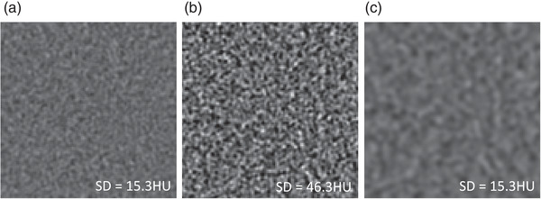
(a) Higher radiation exposure image, (b) lower radiation exposure image, and (c) Gaussian filtering of (b) to match the SD of (a). From the SD alone, it is not possible to distinguish the images of higher and lower radiation exposure images

Noise power spectrum (NPS) can be used to measure both the magnitude and texture of noise and is commonly adopted for evaluation of NRTs. ¹¹ , ¹² , ¹³ The square root of the area under the NPS curve (AUC) shows the noise magnitude, and the shape of the curve represents the noise texture over all spatial frequencies.

When evaluating an NRT using NPS, it is important to evaluate not only the NPS of the denoised images reconstructed with the NRT, but also the NPS of the baseline FBP images without noise reduction. These two NPS curves are compared and the changes in the AUC and NPS‐curve shapes are evaluated for the NRT. However, the comparison of the two NPS curves is normally performed either visually ² , ¹⁴ , ¹⁵ , ¹⁶ or by comparing only the peak or median frequencies. ⁴ , ¹¹ , ¹⁷ , ¹⁸ A visual comparison of the curves cannot on its own provide an objective assessment of noise reduction at each frequency. Similarly, comparing only the peak or median frequency does not capture the full information of NPS because it is only a single value metric.

It is especially challenging to compare NRTs using NPS when the NRTs are from different CT scanners. Each unique CT scanner operating under specific image acquisition conditions will produce baseline FBP images that are also unique. As a result, the optimal starting point for assessment of any NRT is evaluation of the NPS of the denoised image against the NPS of the baseline FBP image. The difficulty with this method then arises when these relative evaluations cannot be compared objectively across the range of NRTs of interest.

For example, Figure 2a,b shows the xy‐plane and z‐direction NPSs of FBP and denoised images obtained from CT scanner #1 with NRT A and CT scanner #2 with NRT B, respectively. As expected, the NPSs of the two baseline FBPs (in blue) are not equivalent because they are derived from two different CT scanners. Therefore, when the objective is to fairly evaluate NRT A relative to NRT B, their respective NPSs from denoised images cannot be compared directly. Instead, the relative differences between each unique set of: (1) baseline FBP NPS and (2) NRT NPS must be compared. But even in this scenario, an objective comparison is still difficult to make using NPS.

FIGURE 2.

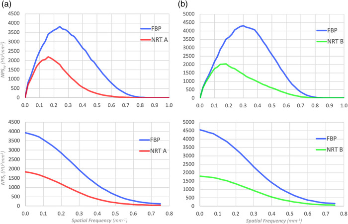
(a) and (b) are two examples of the xy‐plane and z‐directional NPSs of the FBP and NRT images from two different CT scanners. Since the NPSs of the FBP images (blue) are different, it is not possible to simply compare NPSs of NRT A (red) and B (green) to draw conclusion

Figure 3 shows the NPS curves in Figure 2 plotted on a log scale. The difficulty remains in determining whether the two NPS curves are approximately parallel. This determination becomes challenging when the NPS maintains a large curvature. There is no criterion to objectively capture the difference between the two NPS curves in Figure 3.

FIGURE 3.

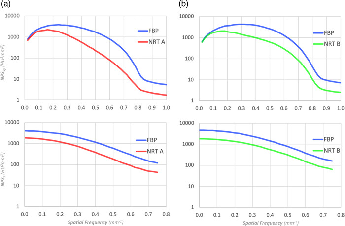
Log scale representation of NPS shown in (a) and (b) of Figure 2. Even with the log scale, it is difficult to objectively recognize the subtle differences between (a) and (b)

To remedy this shortcoming, we recently proposed central frequency ratio (CFR) and noise magnitude ratio (NMR) as metrics for comparing NRTs. ¹⁹ This method has the advantage that an NRT with multiple different settings of noise reduction can be represented by a single performance curve between CFR and NMR, making it possible to compare several NRTs on the same basis. A preferred NRT is the one that maintains CFR while increasing reducing noise, or NMR. However, even with this method, the complexity of NPS is reduced to a single value such as the center of gravity of the NPS over spatial frequency (CFR), thus making it difficult to capture the completeness of the NPS.

In order to further improve the evaluation and comparison of NRTs, it is desirable to objectively visualize the complete degree of noise reduction of each NRT. The primary aim of this work is to propose the new metric of noise reduction profile (NRP) to objectively evaluate NRTs of various CT vendors shown in Table 1.

TABLE 1.

Noise‐reduction techniques for comparison

Manufacturer	Abbreviation	Base Algorithm	Input Data
Canon	AIDR3D	Statistical Iterative Reconstruction	Image and projection
	AiCE	Deep Learning Reconstruction	Projection
GE	ASiR	Statistical Iterative Reconstruction	Image and projection
	ASiR‐V	Hybrid of Statistical and Model‐based Iterative Reconstruction	Image and projection
	TrueFidelity	Deep Learning Reconstruction	Projection
Philips	iDose	Statistical Iterative Reconstruction	Image and projection
Siemens	SAFIRE	Statistical Iterative Reconstruction	Image and projection
	ADMIRE	Model Based Iterative Reconstruction	Image and projection
AlgoMedica	PixelShine	Deep Learning‐based Noise Reduction	Image

A range of NRTs were evaluated, with brief descriptions of each as follows:

• AIDR3D ⁸ , ²⁰ is one of the iterative reconstruction methods offered by Canon Medical Systems (Otawara, Tochigi, Japan), now in its fourth generation. AIDR3D reduces noise by repeating the analysis and processing of data in raw and image data spaces. AiCE ² is Canon's latest reconstruction method using deep learning.

• ASiR ²¹ , ²² is the first generation of statistical iterative reconstructions from GE Healthcare (Waukesha, Wisconsin, USA). ASiR‐V ²³ is the third generation of iterative reconstruction, with improved noise and object modeling compared to ASiR, and a modeling process that incorpoates some of the physical models used in the second generation VEO. ²³ TrueFidelity is a new, state‐of‐the‐art denoising reconstruction based on deep learning.

• iDose ²⁴ , ²⁵ is a fourth‐generation hybrid iterative reconstruction algorithm introduced by Philips Healthcare (Eindhoven, Netherlands). The iterative reconstruction is performed in both the raw and image data spaces.

• SAFIRE ²⁶ is the second generation of iterative reconstructions from Siemens Healthineers (Forchheim, Germany) and is classified as a statistical iterative reconstruction. ADMIRE ²⁷ is the third generation. It utilizes a statistical model of both raw and image data as well as a system model of forward projection, putting it in the category of model‐based iterative reconstructions. ²⁸

• PixelShine ⁶ , ¹⁹ , ²⁹ is a deep learning‐based noise‐reduction from AlgoMedica (Sunnyvale, California, USA). It takes reconstructed CT images as input and operates independently of the vendor, CT model, acquisition conditions, or reconstruction used.

2. MATERIALS AND METHODS

The homogeneous module of the ACR CT phantom (model 464, Gammex‐RMI, Middleton, Wisconsin, USA) or Catphan 500 phantom (The Phantom Laboratory, Salem, New York) was scanned on various CT scanners and reconstructed using FBP and various NRTs. Details of the CT models, reconstruction methods, as well as acquisition and reconstruction conditions are shown in Table 2. The FBP images were baseline images and those reconstructed using the NRTs of ADMIRE, AIDR3D, AiCE, ASiR, ASiR‐V, SAFIRE, TrueFidelity, and iDose were denoised images. For PixelShine, the FBP image at 25 mA was used as baseline, and was processed with all strengths of PixelShine as denoised images. All acquisitions were performed twice to eliminate image background in the NPS calculation.

TABLE 2.

Details of the CT models, reconstruction techniques, as well as acquisition and reconstruction parameters used in this study

Evaluated Algorithms	ADMIRE	AIDR3D/AiCE	ASiR/ASiR‐V	PixelShine	SAFIRE	TrueFidelity	iDose
Phantom	ACR	Catphan	ACR	ACR	ACR	ACR	ACR
Scanner
Vendor	Siemens	Canon	GE	GE	Siemens	GE	Philips
Scanner Model	SOMATOM Force	Aquilion ONE	Revolution HD	Revolution HD	Biograph 64	Revolution CT	iCT 256
Acquisition Conditions
Scan Mode	Helical	Helical	Helical	Helical	Helical	Helical	Helical
Revolution Time	1 s	1 s	0.8 s	0.8 s	1 s	1 s	0.4 s
Total Collimation Width	57.6 mm	40 mm	40 mm	40 mm	19.2 mm	40 mm	40 mm
Single Collimation Width	0.6 mm	0.5 mm	0.625 mm	0.625 mm	1.2 mm	0.625 mm	0.625 mm
Spiral Pitch Factor	1	0.813	0.984	0.984	1	0.984	0.39
Table Feed Per Rotation	57.6 mm/rot	32.5 mm/rot	39.375 mm/rot	39.375 mm/rot	19.2 mm/rot	39.375 mm/rot	24.96 mm/rot
KVP	120 kVp	120 kVp	120 kVp	120 kVp	120 kVp	120 kVp	120 kVp
X Ray Tube Current	23 mA	30 mA	25 mA	25 mA	20 mA	20 mA	24 mA
Effective mAs	20.3 mAs	36.9 mAs	20.3 mAs	20.3 mAs	24.6 mAs	20 mAs	23 mAs
Filter Type	FLAT	LARGE	MEDIUM FILTER	MEDIUM FILTER	FLAT	HEAD FILTER	UB
Data Collection Diameter	500 mm	500 mm	320 mm	320 mm	500 mm	320 mm	500 mm
CTDIvol (Body 32)	1.4 mGy	1.9 mGy	1.5 mGy	1.5 mGy	1.3 mGy	1.1 mGy	1.5 mGy
Reconstruction ‐ Baseline Images
Reconstruction Algorithm	FBP	FBP	FBP	FBP	FBP	FBP	FBP
Convolution Kernel	Hr40s	FC13	STANDARD	STANDARD	H40s	STANDARD	UB
Reconstruction Diameter	250 mm	250 mm	250 mm	250 mm	250 mm	250 mm	250 mm
Thickness	2.0 mm	2.0 mm	2.5 mm	2.5 mm	2.0 mm	2.0 mm	2.5 mm
Matrix Size	512 x 512	512 x 512	512 x 512	512 x 512	512 x 512	512 x 512	512 x 512
Reconstruction ‐ Denoised Images
Reconstruction Algorithm	ADMIRE	AIDR3D/AiCE	ASiR/ASiR‐V	–	SAFIRE	TrueFidelity	iDose
Convolution Kernel	Hr40s	FC13/BodySharp	STANDARD	–	J40s	STANDARD	UB
Reconstruction Diameter	250 mm	250 mm	250 mm	–	250 mm	250 mm	250 mm
Thickness	2.0 mm	2.0 mm	2.5 mm	–	2.0 mm	2.0 mm	2.5 mm
Matrix Size	512 x 512	512 x 512	512 x 512	–	512 x 512	512 x 512	512 x 512

2.1. Calculation of NPS

We used the method of Friedman et al. ³⁰ to calculate NPS. As shown in Figure 4, 12 square cuboids of 128 pixels $\times$ 128 pixels $\times$ 21 slices were extracted from the difference of the phantom images acquired consecutively (twice) to remove the background of the image, and 3D Fast Fourier Transform was applied to each of them. The ensemble mean of the squares of the corresponding voxel values was then calculated and divided by two for the 3D NPS. As shown in Figure 5, the rotational mean of the 3D NPS in the z‐axis direction was calculated and its radial profile was defined as NPS_xy and its z‐axis profile as NPS_z .

FIGURE 4.

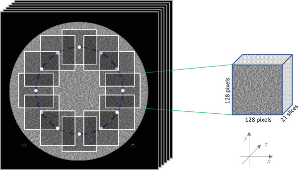
Extracted 12 square cuboids from the phantom images

FIGURE 5.

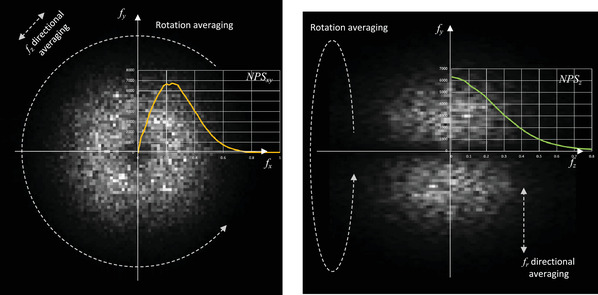
Calculation of NPS_xy and NPS_z from 3D NPS

2.2. Definition of Noise Reduction Profile

Let $NP{S}_{xy,NRT}(f)$ be the NPS in the xy‐plane of a denoised image by an NRT, and let $NP{S}_{xy,FBP}(f)$ be the NPS of an FBP image, where f is the spatial frequency. Then $NR{P}_{xy}(f)$ is the noise reduction profile of the NRT, and is defined as

$$\begin{array}{ccc}\hfill NR{P}_{xy}(f)& =& \log \left(NP{S}_{xy,FBP}(f)\right)-\log \left(NP{S}_{xy,NRT}(f)\right)\hfill \\ & =& \log \left(\frac{NP{S}_{xy,FBP}(f)}{NP{S}_{xy,NRT}(f)}\right),\hfill \end{array}$$ (1)

a logarithmic scale of the noise‐reduction rate per spatial frequency f.

Similarly, for the z‐axis direction, $NR{P}_z(f)$ is defined as

$$\begin{array}{ccc}\hfill NR{P}_z(f)& =& \log \left(NP{S}_{z,FBP}(f)\right)-\log \left(NP{S}_{z,NRT}(f)\right)\hfill \\ & =& \log \left(\frac{NP{S}_{z,FBP}(f)}{NP{S}_{z,NRT}(f)}\right),\hfill \end{array}$$ (2)

where $NP{S}_{z,NRT}(f)$ and $NP{S}_{z,FBP}(f)$ are the z‐axis NPS of the denoised and FBP images, respectively.

2.3. Physical meaning of NRP

NRP of an NRT is the log scale of the noise reduction ratio at each spatial frequency. The log scale is to reduce the dynamic range when comparing different DRTs. When calculating NRP, it is critical to use the same kernel for the reconstructions with and without NRT to prevent factors other than noise reduction from appearing in the NRP. Reconstruction kernel selection affects the shape of NPS because each kernel is a filter, which is in general a linear operator. For instance, a soft kernel (or low‐pass filter) shifts the NPS curve toward a lower frequency, while a lung filter (or high‐pass filter) shifts the NPS curve toward a higher frequency. Therefore, if different kernels are selected to reconstruct denoised and FBP images, both the difference in noise components due to NRT and the frequency processing due to the usage of different kernels will be included in the NRP. In this scenario, the noise reduction characteristics of the NRT cannot be calculated correctly. To our knowledge, Canon's AiCE and FIRST, GE's VEO, and Siemens’ SAFIRE do not provide the same kernels of FBP in their corresponding NRTs. Hence, when calculating NRP for these NRTs, the most similar kernels should be selected for the reconstruction of the denoised and FBP images. For some vendors, it is straightforward to find similar kernels for NRT and FBP. For example, in Siemens, if two kernels are with the same number, then they are of similar kernel. If the similar kernels are not explicit, the best way to find out for sure is to contact the vendor.

3. RESULTS

Figures 6 and 7 show the xy plane and z‐axis NRP curves of the NRTs in Table 1. For reference, the corresponding NPS curves are also shown in Figure 6. In NRP and NPS, graphs with the same intensity at each NRT are shown in the same color. The NRP curves in both figures are (a) ADMIRE, (b) AIDR3D, (c) ASiR, (d) ASiR‐V, (e) AiCE, (f) PixelShine, (g) SAFIRE, (h) TrueFidelity, and (i) iDose. For each NRT, NRP curves for all the strengths of noise reduction are plotted together in a single graph. These graphs clearly show that each NRT has its own uniquely shaped NRP curves, which were not readily discernable in the NPS curves.

FIGURE 6.

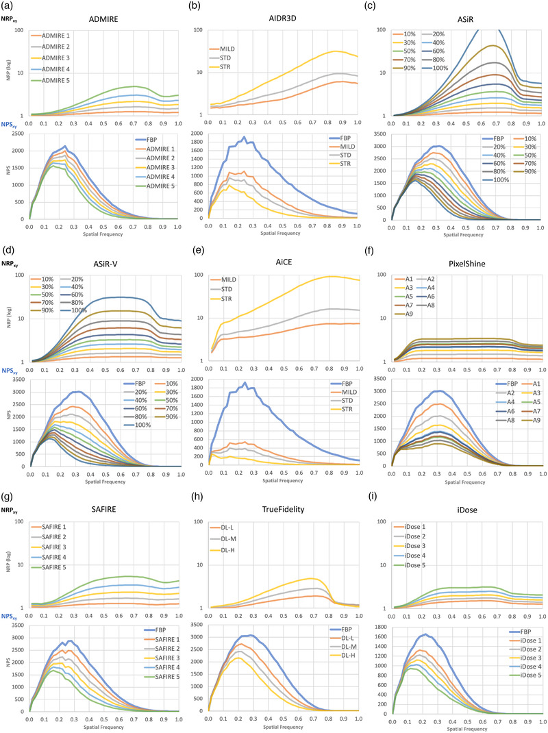
NRP (top) and NPS (bottom) for each NRT in the xy‐plane; (a) ADMIRE, (b) AIDR3D, (c) ASiR, (d) ASiR‐V, (e) AiCE, (f) PixelShine, (g) SAFIRE, (h) TrueFidelity, and (i) iDose

FIGURE 7.

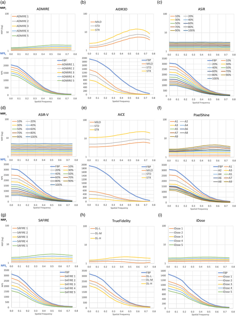
NRP (top) and NPS (bottom) for each NRT in the z direction; (a) ADMIRE, (b) AIDR3D, (c) ASiR, (d) ASiR‐V, (e) AiCE, (f) PixelShine, (g) SAFIRE, (h) TrueFidelity, and (i) iDose

Figure 6a shows the NRP and NPS of ADMIRE in the xy‐plane, and Figure 7a shows the NRP of ADMIRE in the z‐direction. The NRP of ADMIRE rises slowly and has a gentle peak around 0.7. The slope of the increasing NRP becomes larger as the strength of ADMIRE increases. Observing the corresponding NPS, the NPS peak shifts to the lower frequency side with the increasing strength of ADMIRE. As for the z‐direction, the curve is slightly curved, but almost constant.

The peaks of the NRPs of AIDR3D are around the spatial frequency of 0.85 mm^–1 in Figure 6b, and the noise reduction rate is almost proportional to the increase of spatial frequency up to 0.85 mm^–1. The slope of the rising NRP of AIDR3D varies slightly depending on the strength of AIDR3D, but the slope is relatively large even at the weakest strength. In the z‐direction (Figure 7b), the NRPs are bell‐shaped curves around the spatial frequency of 0.6 mm^–1, exhibiting a larger change over the spatial frequencies than the other NRTs, whose NRPs in the z‐direction are almost constant.

Figures 6c and 7c show the NRPs of ASiR. The difference in noise reduction rate between low and high frequencies at the strongest intensity in the xy‐direction is the largest compared to the other NRTs. After 0.8 mm^–1 where the NPS is close to zero, it drops sharply. On the other hand, the NRP in the z‐direction is constant for all frequencies.

Figures 6d and 7d show the NRP of ASiR‐V in the xy and z directions. The NRP in the xy plane increases from 0 to 0.4 mm⁻¹ and then becomes almost constant between 0.4 and 0.8 mm⁻¹. As in ASiR, there is a large difference in the noise reduction rate between the low and high frequency regions at strong strength, but the noise reduction rate at the high frequency side of the NRP is smaller than that of ASiR. In the z direction, the NRP is flat, as in ASiR.

As shown in Figure 6e, the NRPs of AiCE increase rapidly between 0 and 0.1 mm⁻¹ and then gradually increase towards 0.8 to 1.0 mm⁻¹. For the STRONG setting, there is a large difference in the noise reduction rate between the low and high frequency regions. However, for the MILD setting, the NRP is almost constant after 0.1 mm⁻¹. On the other hand, as shown in Figure 7e, the z‐axis NRPs are not flat, but has a slight curve.

As shown in Figure 6f, the NRPs of PixelShine increase between 0 and 0.15 mm^–1, and then remain constant up to 0.8 mm^–1. After 0.8 mm^–1 where the NPS is close to zero, they decrease slightly . On the other hand, as shown in Figure 7f, the z‐axis NRP is flat for the strengths of A1–A5, whereas the gentle bell‐shaped curves with peaks around 0.6 mm^–1 are observed above A6.

The NRP in the xy‐plane of SAFIRE in Figure 6g is similar to that of ADMIRE in (a). The slope of the tangent line of the NRP around 0.25 mm⁻¹ is larger for SAFIRE than for ADMIRE. On the other hand, the z‐direction NRP of SAFIRE in Figure 7g has a larger curve shape than that of ADMIRE.

The xy‐plane NRPs for TrueFidelity show curves with peaks around 0.7 mm^–1 and steep declines above 0.7 mm^–1 where the NPS is close to zero, as shown in Figure 6h. The slopes of the curves become steeper as the strength increases, although even at the strength H (high), the difference between the low and high frequency ranges is smaller than those of ASiR and ASiR‐V. On the other hand, the NRPs in the z‐direction show relatively flat curves with different peak positions depending on the strength (Figure 7h).

Next, as shown in Figure 6i, the NRPs in the xy‐plane of iDose slowly increase between 0 and 0.3 mm^–1, flatten up to about 0.7 mm^–1, and then decrease slightly above 0.7 mm^–1 where the NPS is close to zero. As shown in Figure 7i, the NRPs in the z‐direction are almost flat with a slight curvature.

4. DISCUSSIONS

In order to understand the NRPs obtained in Figures 6 and 7, we examined the NRPs of three simple noise reduction approaches of scanning at a high radiation dose, smoothing in the xy‐plane with a two‐dimensional Gaussian filter and smoothing in the z‐axis (table direction) with a one‐dimensional Gaussian filter. These are all linear noise reduction methods, different from the nonlinear NRTs in Table 1. It is useful to interpret the behavior of the nonlinear methods in comparison to those of the linear methods, which are more readily and easily understood.

In the method of noise reduction by increasing radiation dose, images were acquired at 25 mA as a baseline, and then at 50, 75, 100, and 150 mA (all considered denoised images). All images were reconstructed with FBP. The NPS and NRP are in Figure 8a. There is no shift of the frequencies for the peaks of the NPS in the xy‐plane. It is difficult to determine if a shift has occurred because there is no peak for the NPS in the z‐axis direction. The NRP on the xy‐plane is constant in the range of 0–0.8 mm^–1, and decreases slightly after 0.8 mm^–1 where the NPS is almost zero. The NRP in the z‐axis direction was also constant in the entire range of spatial frequencies.

FIGURE 8.

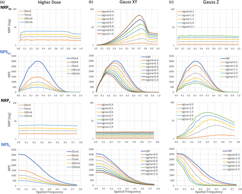
From top, NRP and NPS in the xy‐plane and the z‐direction, respectively, when noise is reduced by (a) scanning with higher radiation doses, (b) applying a two‐dimensional Gaussian filter in the xy‐plane, and (c) applying a one‐dimensional Gaussian filter in the z‐axis. The NRPs are constant in both the xy and z directions when the images are captured with higher radiation doses

In noise reduction by two‐dimensional Gaussian filtering in the xy‐plane (GaussXY), a Gaussian filter with σ = 0.4 to 1.0 pixels was applied to a baseline 25 mA FBP image for a denoised image. The noise texture is smoothed only in the xy plane, and it is smoothed more by a large σ. There is no impact to the z‐direction. Figure 8b shows the NPS and NRP in the xy‐plane and z‐direction, and the NPS peak shifts to the left with σ only in the xy‐plane. Again it is difficult to determine the NPS in the z‐axis direction because there is no peak. The NRP in the xy‐plane increases between 0 and 0.7 mm^–1, reaches a peak between 0.7 and 0.75 mm^–1, and then decreases after 0.75 mm^–1 where the NPS is close to zero. Furthermore, between 0 and 0.7 mm^–1, the slope of NRP increases as σ increases. In contrast, the NRP in the z‐direction is constant over all frequencies.

Gaussian filtering along the z‐axis (GaussZ) with σ = 0.5 to 2.5 slices was applied to the baseline 25 mA FBP image for a denoised image. This is equivalent to denoising by image reconstruction of thicker slices, which reduces noise in the xy‐plane. Figure 8c shows the NPS and NRP in the xy‐plane and z‐direction. In the NPS, there is no shift of the peaks in the xy‐plane, but in the z‐axis, the entire NPS curve is shifted to a lower frequency. The NRP in the xy‐plane is constant for all frequencies. In the z‐direction, The NRP in the z‐direction has a peak around the spatial frequency of 0.4–0.6 mm^–1, and the slope from 0 to the peak becomes larger as σ increases.

4.1. Relationship between NRP and NPS

From Figures 6 and 8, there is a direct relationship between the shape of the NRP curve and the shift of the NPS peak position. Here we derive the relationship for the case where only one peak exists in the NPS of the xy plane.

Let $NP{S}_{FBP}(f)$ be the NPS of the image without noise reduction, and be a function with one peak at $f=a(a>0)$, differentiable for $f>0$, monotonically increasing for $f<a$, and monotonically decreasing for $f>a$. Similarly, let $NP{S}_{NRT}(f)$ be the NPS of the image after noise reduction, with one peak at $f=b(b>0)$, differentiable for $f>0$, monotonically increasing for $f<b$, and monotonically decreasing for $f>b$. From these conditions,

$$NP{S}_{FBP}^{\prime }(a)=0,\mathrm{and}NP{S}_{NRT}^{\prime }(b)=0.$$

Here, from Equation (1), $NRP(f)$ can be expressed as

$$\begin{array}{ccc}\hfill NRP(f)& =& \log \left(\frac{NP{S}_{FBP}(f)}{NP{S}_{NRT}(f)}\right)\hfill \\ & =& \log \left(h(f)\right).\hfill \end{array}$$

Then,

$$\begin{array}{c}\hfill NP{S}_{FBP}(f)=h(f)NP{S}_{NRT}(f).\end{array}$$

From the Product Rule of calculus,

$$\begin{array}{ccc}\hfill NP{S}_{FBP}^{\prime }\left(a\right)& =& h^{\prime }\left(a\right)NP{S}_{NRT}\left(a\right)+h\left(a\right)NP{S}_{NRT}^{\prime }\left(a\right)=0\hfill \\ \hfill NP{S}_{NRT}^{\prime }\left(a\right)& =& -\frac{NP{S}_{NRT}\left(a\right)}{h\left(a\right)}{h}^{\prime }\left(a\right).\hfill \end{array}$$

Here, $NP{S}_{NRT}(f)>0$ and $h(f)>0$, there are three possible values for $NP{S}_{NRT}^{\prime }(a)$.

1. When $h^{\prime }(a)>0$, $NP{S}_{NRT}^{{}^{\prime }}(a)<0$. The slope of the tangent line of $NP{S}_{NRT}(f)$ at $f=a$ is negative, and $NP{S}_{NRT}(f)$ has a decreasing trend at $f=a$. Here, $NP{S}_{NRT}(f)$ has one peak at $f=b(b>0)$. It is differentiable for $f>0$, monotonically increasing for $f<b$ and monotonically decreasing for $f>b$. This leads to $a>b$.

• Therefore, when $h^{\prime }(a)>0$, the peak position of $NP{S}_{NRT}(f)$, $f=b$, is shifted to the lower frequency side than the peak position of $NP{S}_{FBP}(f)$, $f=a$.

• b.When $h^{\prime }(a)=0$, $NP{S}_{NRT}^{\prime }(a)=0$. In this case, $a=b$. When $h^{\prime }(a)=0$, the peak position of $NP{S}_{NRT}(f)$ is the same as the peak position of $NP{S}_{FBP}(f)$.
• c.When $h^{\prime }(a)<0$, $NP{S}_{NRT}^{\prime }(a)>0$. The peak position $f=b$ of $NP{S}_{NRT}(f)$ is shifted to the high frequency side than the peak position $f=a$ of $NP{S}_{FBP}(f)$.

Here, because $NRP(f)=\log (h(f))$,

$$NR{P}^{{}^{\prime }}(f)=\frac{h^{\prime }(f)}{h(f)}.$$

Since $h(f)>0$, the sign of $NR{P}^{\prime }(f)$ always matches that of $h^{\prime }(f)$.

In summary, at the peak position $f=a$ of $NP{S}_{FBP}(f)$,

• when $NR{P}^{{}^{\prime }}(a)$>０, the peak position of $NP{S}_{NRT}(f)$ is shifted to the lower frequency side than the peak position of $NP{S}_{FBP}(f)$;

• when $NR{P}^{{}^{\prime }}(a)=0$, the peak position of $NP{S}_{NRT}(f)$ matches the peak position of $NP{S}_{FBP}(f)$;

• when $NR{P}^{{}^{\prime }}(a)<0$, the peak position of $NP{S}_{NRT}(f)$ is shifted to the higher frequency side than the peak position of $NP{S}_{FBP}(f)$.

The mathematically derived relationship can be confirmed in Figure 6, where the blue color curve in the NPS represents $NP{S}_{FBP}(f)$. From the slope of NRP at the peak position of the NPS, we found that the slope of NRP is close to zero for AiCE MILD and PixelShine at all strengths. The peak positions of these NPSs are not shifted from the ones of the FBP NPSs. For the other NRTs, the slope of the NRP at the peak position of the NPS of FBP is positive, and the peak position of the NPS is shifted to the lower frequency side.

Although the slopes of the NRPs at the peak positions of the NPSs before noise reduction are zero for AiCE MILD and PixelShine, they are clearly different from the higher dose imaging in Figure 8, where the NRPs are constant over the entire spatial frequencies. Therefore, we investigated the central frequencies before and after noise reduction by scanning at higher radiation doses for AiCE MILD, and PixelShine. The results are shown in Table 3. The central frequency does not shift at higher radiation dose levels. However, the central frequencies shift with AiCE MILD and PixelShine even though there is no change in the peak position of NPS. It is possible that if the NRPs are not completely constant, a shift in the central frequency of the NPS may occur even if there is no shift of the peak position in NPS. The proof is shown in the Appendix.

TABLE 3.

Center frequencies (mm⁻¹) of baseline and denoised images. The central frequency does not shift at higher radiation dose levels. However, the central frequencies shift with AiCE MILD and PixelShine even though there is no change at the peak position of NPS

Higher Dose		AiCE		PixelShine
	Central frequency		Central frequency		Central frequency
Baseline	0.329	Baseline	0.356	Baseline	0.329
50 mA	0.329	MILD	0.317	A1	0.326
75 mA	0.326			A2	0.323
100 mA	0.329			A3	0.319
150 mA	0.324			A4	0.316
				A5	0.312
				A6	0.315
				A7	0.312
				A8	0.309
				A9	0.305

4.2. Comparison by NRP

Calculating NRP facilitates the comparison of NRTs, even when their FBP images are different. For example, Figure 9 shows the NRP curves for the two NRTs shown in (a) and (b) of Figure 2. Each NRT can be represented by a single curve, and the NRP as a function of spatial frequency becomes apparent at a glance. In addition, even subtle differences become noticeable, as can be seen from the z‐axis NRPs.

FIGURE 9.

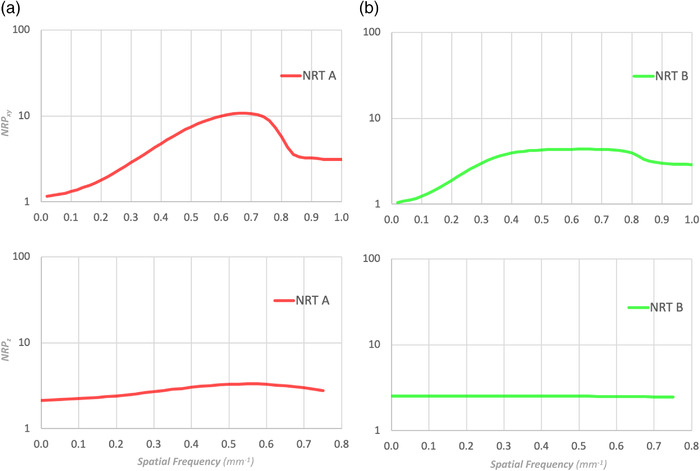
The xy‐plane and z‐axis NRP of the NRTs in Figure 2: (a) NRT A and (b) NRT B. The two NRPs can be compared even when the NPS of the FBP images are different

It is important to understand that there are theoretical limitations to using NPS for evaluating and comparing NRTs. The definition of NPS assumes linearity of the system and stationarity of the noise, which may be invalidated in situations where nonlinear algorithms are used for image reconstruction and denoising. It is still possible, however, that the NPS can serve as one of qualitative metrics to assess the quality of CT systems using nonlinear reconstruction techniques.

In addition, it should be noted that all of the NRTs shown in Table 1 are nonlinear, so the noise reduction properties may depend on parameters such as radiation dose, convolution kernel, and FOV. When attempting to make direct comparisons, it is important to pay attention to these parameters.

Finally, when computing the NRP, it is important to use the same kernel with and without NRT. Canon's AiCE and FIRST and Siemens' SAFIRE do not use the same kernel as FBP. The most similar kernel should be selected to reconstruct the denoised and FBP images when calculating the NRP.

5. CONCLUSIONS

We proposed a new metric, the noise reduction profile (NRP), for evaluating and comparing NRTs in CT imaging. We calculated the NRP curves for most of the commercially available NRTs and demonstrated that each NRT has its own unique NRP. Furthermore, the relationship between the shape of the NRP and the shifts in NPS due to application of NRTs was mathematically clarified. The NRP facilitates objective comparison of the detailed noise reduction properties of each NRT over all relevant spatial frequencies.

CONFLICT OF INTEREST

Dr. Akira Hasegawa is an employee of AlgoMedica, Inc. and Dr. Tinsu Pan is a consultant for Bracco Diagnostic, Inc.

RELATIONSHIP BETWEEN NRP AND NPS CENTRAL FREQUENCY SHIFT

Let $NP{S}_{FBP}(f)$ be the NPS of the image before noise reduction, and let $NP{S}_{FBP}(f)>0$ and differentiable for $f>0$. Similarly, let $NP{S}_{NRT}(f)$ be the NPS of the image after noise reduction by a NRT, and let $NP{S}_{NRT}(f)>0$ and differentiable for $f>0$.

From Equation (1), $NRP(f)$ can be expressed as

$$\begin{array}{ccc}\hfill NRP(f)& =& \log \left(\frac{NP{S}_{FBP}(f)}{NP{S}_{NRT}(f)}\right)\hfill \\ & =& \log \left(h(f)\right).\hfill \end{array}$$

Then,

$$\begin{array}{c}NP{S}_{FBP}(f)=h(f)·NP{S}_{NRT}(f).\end{array}$$ (A1)

Let the area under $NP{S}_{FBP}(f)$ be $S_{FBP}$ and the area under $NP{S}_{NRT}(f)$ be $S_{NRT}$. Then the central frequency of $NP{S}_{FBP}(f)$, $C{F}_{FBP}$ is

$$C{F}_{FBP}=\frac{1}{S_{FBP}}\underset{0}{\overset{1}{\int }}f·NP{S}_{FBP}(f)df.$$

From Equation (A1),

$$C{F}_{FBP}=\frac{1}{S_{FBP}}\underset{0}{\overset{1}{\int }}f·h(f)·NP{S}_{NRT}(f)df.$$

Here, by describing

$$\begin{array}{c}\hfill G(f)=\underset{}{\stackrel{}{\int }}f·\mathrm{NP}{S}_{\mathrm{NRT}}(f)\mathrm{df},\end{array}$$ (A2)

and using Integration by parts, we get

$$\begin{array}{ccc}\hfill C{F}_{FBP}& =& \frac{1}{S_{FBP}}\left\{{\left[G(f)·h(f)\right]}_0^1-{\int }_0^{1}G(f)·h^{\prime }(f)df\right\}\hfill \\ & =& \frac{1}{S_{FBP}}\{G\left(1\right)·h\left(1\right)-G\left(0\right)·h\left(0\right)\hfill \\ & & -\underset{0}{\overset{1}{\int }}G(f)·h^{\prime }(f)df\}.\hfill \end{array}$$ (A3)

Now, from Equation (A2),

$$\underset{0}{\overset{1}{\int }}f·NP{S}_{NRT}(f)df=G\left(1\right)-G\left(0\right),$$

and then,

$$G\left(1\right)=\underset{0}{\overset{1}{\int }}f·NP{S}_{NRT}(f)df+G\left(0\right).$$

Substituting this into Equation (A3), we get

$$\begin{array}{ccc}\hfill C{F}_{FBP}& =& \frac{1}{S_{FBP}}\{h\left(1\right)\underset{0}{\overset{1}{\int }}f·NP{S}_{NRT}(f)df+G\left(0\right)·h\left(1\right)\hfill \\ & & -G\left(0\right)·h\left(0\right)-\underset{0}{\overset{1}{\int }}G(f)·h^{\prime }(f)df\}\hfill \\ & =& \frac{h\left(1\right)}{S_{FBP}}·S_{NRT}·\frac{1}{S_{NRT}}\underset{0}{\overset{1}{\int }}f·NP{S}_{NRT}(f)df\hfill \\ & & +\frac{G\left(0\right)}{S_{FBP}}\left[h\left(1\right)-h\left(0\right)\right]-\frac{1}{S_{FBP}}\underset{0}{\overset{1}{\int }}G(f)·h^{\prime }(f)df\hfill \\ & =& \frac{S_{NRT}}{S_{FBP}}·h\left(1\right)·C{F}_{NRT}+\frac{G\left(0\right)}{S_{FBP}}\left[h\left(1\right)-h\left(0\right)\right]\hfill \\ & & -\frac{1}{S_{FBP}}\underset{0}{\overset{1}{\int }}G(f)·h^{\prime }(f)df\hfill \end{array}$$ (A4)

Here, when $h(f)=k$,

$$\begin{array}{ccc}\hfill h\left(1\right)& =& h\left(0\right)=k,\hfill \\ \hfill h^{\prime }(f)& =& 0.\hfill \end{array}$$

Therefore, the second and third terms in Equation (A4) are both zero, and

$$C{F}_{FBP}=\frac{S_{NRT}}{S_{FBP}}·k·C{F}_{NRT}.$$ (A5)

Here, because of $NP{S}_{FBP}(f)=k·NP{S}_{NRT}(f),$

$$\begin{array}{ccc}\hfill \underset{0}{\overset{1}{\int }}NP{S}_{FBP}(f)df& =& \underset{0}{\overset{1}{\int }}k·NP{S}_{NRT}(f)df\hfill \\ & =& k\underset{0}{\overset{1}{\int }}NP{S}_{NRT}(f)df.\hfill \end{array}$$

Then,

$$\begin{array}{ccc}\hfill S_{FBP}& =& k·S_{NRT}\hfill \\ \hfill k& =& \frac{S_{FBP}}{S_{NRT}}.\hfill \end{array}$$

Substituting this into Equation (A5), we get

$$\begin{array}{ccc}\hfill C{F}_{FBP}& =& \frac{S_{NRT}}{S_{FBP}}·k·C{F}_{NRT}\hfill \\ & =& \frac{S_{NRT}}{S_{FBP}}·\frac{S_{FBP}}{S_{NRT}}·C{F}_{NRT}\hfill \\ & =& C{F}_{NRT}.\hfill \end{array}$$

When $NRP(f)$ is constant over $f$, the central frequencies of $NP{S}_{FBP}(f)$ and $NP{S}_{NRT}(f)$ coincide. When $NRP(f)$ is not constant, the second and third terms in Equation (A4) are not zero, and the central frequencies of $NP{S}_{FBP}(f)$ and $NP{S}_{NRT}(f)$ may not coincide.

Hasegawa A, Ishihara T, Thomas MA, Pan T. Noise reduction profile: A new method for evaluation of noise reduction techniques in CT. Med Phys. 2022;49:186–200. 10.1002/mp.15382

DATA AVAILABILITY STATEMENT

Data sharing is not applicable to this article as no new data were created or analyzed in this study.

REFERENCES

- 1. Padole A, Ali Khawaja RD, Kalra MK, Singh S. CT radiation dose and iterative reconstruction techniques. Am J Roentgenol. 2015;204(4):W384‐W392. [DOI] [PubMed] [Google Scholar]
- 2. Higaki T, Nakamura Y, Zhou J, et al. Deep learning reconstruction at CT: phantom study of the image characteristics. Acad Radiol. 2020;27(1):82‐87. [DOI] [PubMed] [Google Scholar]
- 3. Racine D, Becce F, Viry A, et al. Task‐based characterization of a deep learning image reconstruction and comparison with filtered back‐projection and a partial model‐based iterative reconstruction in abdominal CT: a phantom study. Phys Med. 2020;76:28‐37. [DOI] [PubMed] [Google Scholar]
- 4. Shin YJ, Chang W, Ye JC, et al. Low‐dose abdominal CT using a deep learning‐based denoising algorithm: a comparison with CT reconstructed with filtered back projection or iterative reconstruction algorithm. Korean J Radiol. 2020;21(3):356. [DOI] [PMC free article] [PubMed] [Google Scholar]
- 5. Willemink MJ, Noël PB. The evolution of image reconstruction for CT—from filtered back projection to artificial intelligence. Eur Radiol. 2019;29(5):2185‐2195. [DOI] [PMC free article] [PubMed] [Google Scholar]
- 6. Tian S, Liu A, Liu J, Liu Y, Pan J. Potential value of the PixelShine deep learning algorithm for increasing quality of 70 kVp+ASiR‐V reconstruction pelvic arterial phase CT images. Jpn J Radiol. 2018;37(2):186‐190. [DOI] [PubMed] [Google Scholar]
- 7. Leipsic J, LaBounty TM, Heilbron B, et al. Adaptive statistical iterative reconstruction: assessment of image noise and image quality in coronary CT angiography. Am J Roentgenol. 2010;195(3):649‐654. [DOI] [PubMed] [Google Scholar]
- 8. Joemai RMS, Veldkamp WJH, Kroft LJM, Hernandez‐Giron I, Geleijns J. Adaptive iterative dose reduction 3D versus filtered back projection in CT: evaluation of image quality. Am J Roentgenol. 2013;201(6):1291‐1297. [DOI] [PubMed] [Google Scholar]
- 9. Geyer LL, Schoepf UJ, Meinel FG, et al. State of the art: iterative CT reconstruction techniques. Radiology. 2015;276(2):339‐357. [DOI] [PubMed] [Google Scholar]
- 10. Mileto A, Guimaraes LS, McCollough CH, Fletcher JG, Yu L. State of the art in abdominal CT: the limits of iterative reconstruction algorithms. Radiology. 2019;293(3):491‐503. [DOI] [PubMed] [Google Scholar]
- 11. Greffier J, Larbi A, Frandon J, Moliner G, Beregi JP, Pereira F. Comparison of noise‐magnitude and noise‐texture across two generations of iterative reconstruction algorithms from three manufacturers. Diagn Interv Imaging. 2019;100(7‐8):401‐410. [DOI] [PubMed] [Google Scholar]
- 12. Samei E, Richard S. Assessment of the dose reduction potential of a model‐based iterative reconstruction algorithm using a task‐based performance metrology: CT task‐based performance metrology. Med Phys. 2014;42(1):314‐323. [DOI] [PubMed] [Google Scholar]
- 13. Ehman EC, Yu L, Manduca A, et al. Methods for clinical evaluation of noise reduction techniques in abdominopelvic CT. RadioGraphics. 2014;34(4):849‐862. [DOI] [PubMed] [Google Scholar]
- 14. Li G, Liu X, Dodge CT, Jensen CT, Rong XJ. A noise power spectrum study of a new model‐based iterative reconstruction system: veo 3.0. J Appl Clin Med Phys. 2016;17(5):428‐439. [DOI] [PMC free article] [PubMed] [Google Scholar]
- 15. Holmquist F, Nyman U, Siemund R, Geijer M, Söderberg M. Impact of iterative reconstructions on image noise and low‐contrast object detection in low kVp simulated abdominal CT: a phantom study. Acta Radiol. 2016;57(9):1079‐1088. [DOI] [PubMed] [Google Scholar]
- 16. Mirro AE, Brady SL, Kaufman RA. Full dose‐reduction potential of statistical iterative reconstruction for head CT protocols in a predominantly pediatric population. Am J Neuroradiol. 2016;37(7):1199‐1205. [DOI] [PMC free article] [PubMed] [Google Scholar]
- 17. Kataria B, Nilsson Althén J, Smedby Ö, Persson A, Sökjer H, Sandborg M. Assessment of image quality in abdominal computed tomography: effect of model‐based iterative reconstruction, multi‐planar reconstruction and slice thickness on potential dose reduction. Eur J Radiol. 2020;122:108703. [DOI] [PubMed] [Google Scholar]
- 18. Suzuki S, Katada Y, Takayanagi T, et al. Evaluation of three‐dimensional iterative image reconstruction in C‐arm‐based interventional cone‐beam CT: a phantom study in comparison with customary reconstruction technique. Medicine (Baltimore). 2019;98(13):e14947. [DOI] [PMC free article] [PubMed] [Google Scholar]
- 19. Pan T, Hasegawa A, Luo D, Wu CC, Vikram R. Technical Note: impact on central frequency and noise magnitude ratios by advanced CT image reconstruction techniques. Med Phys. 2020;47(2):480‐487. [DOI] [PubMed] [Google Scholar]
- 20. Angel E, AIDR 3D Iterative Reconstruction: integrated, automated and adaptive dose reduction. 2012. https://us.medical.canon/download/aidr‐3d‐wp‐aidr‐3d. Accessed December 4, 2021.
- 21. Hara AK, Paden RG, Silva AC, Kujak JL, Lawder HJ, Pavlicek W. Iterative reconstruction technique for reducing body radiation dose at CT: feasibility Study. Am J Roentgenol. 2009;193(3):764‐771. [DOI] [PubMed] [Google Scholar]
- 22. Nuyts J, Man BD, Dupont P, Defrise M, Suetens P, Mortelmans L. Iterative reconstruction for helical CT: a simulation study. Phys Med Biol. 1998;43(4):729‐737. [DOI] [PubMed] [Google Scholar]
- 23. Fan J, Yue M, Melnyk R, Benefits of ASiR‐V reconstruction for reducing patient radiation dose and preserving diagnostic quality in CT exams. https://www.gehealthcare.co.uk/‐/media/6862ed3b10424182924e03a49f4a46d7.pdf. Accessed December 4, 2021.
- 24. iDose iterative reconstruction technique . 2011. http://incenter.medical.philips.com/doclib/enc/fetch/2000/4504/577242/577249/586938/587315/iDose4_‐_Whitepaper_‐_Technical_‐Low_Res.pdf%3fnodeid%3d8432599%26vernum%3d‐2. Accessed December 4, 2021.
- 25. Arapakis I, Efstathopoulos E, Tsitsia V, et al. Using “iDose4” iterative reconstruction algorithm in adults’ chest–abdomen–pelvis CT examinations: effect on image quality in relation to patient radiation exposure. Br J Radiol. 2014;87(1036). [DOI] [PMC free article] [PubMed] [Google Scholar]
- 26. Grant K, Raupach R, SAFIRE: sinogram affirmed iterative reconstruction. https://cdn0.scrvt.com/39b415fb07de4d9656c7b516d8e2d907/1800000000306520/d80046026fd1/ct_SAFIRE_White_Paper_1800000000306520.pdf. Accessed December 4, 2021.
- 27. Ellmann S, Kammerer F, Allmendinger T, et al. Advanced modeled iterative reconstruction (ADMIRE) facilitates radiation dose reduction in abdominal CT. Acad Radiol. 2018;25(10):1277‐1284. [DOI] [PubMed] [Google Scholar]
- 28. Solomon J, Mileto A, Ramirez‐Giraldo JC, Samei E. Diagnostic performance of an advanced modeled iterative reconstruction algorithm for low‐contrast detectability with a third‐generation dual‐source multidetector CT scanner: potential for radiation dose reduction in a multireader study. Radiology. 2015;275(3):735‐745. [DOI] [PubMed] [Google Scholar]
- 29. Yanagawa M, Niioka H, Hata A, et al. Application of deep learning (3‐dimensional convolutional neural network) for the prediction of pathological invasiveness in lung adenocarcinoma: a preliminary study. Medicine (Baltimore). 2019;98(25):e16119. [DOI] [PMC free article] [PubMed] [Google Scholar]
- 30. Friedman SN, Fung GSK, Siewerdsen JH, Tsui BMW. A simple approach to measure computed tomography (CT) modulation transfer function (MTF) and noise‐power spectrum (NPS) using the American College of Radiology (ACR) accreditation phantom: cT MTF/NPS calculation using an ACR phantom. Med Phys. 2013;40(5):051907. [DOI] [PMC free article] [PubMed] [Google Scholar]
Associated Data
This section collects any data citations, data availability statements, or supplementary materials included in this article.