Analysis of agricultural greenhouse gas emissions using the STIRPAT model: a case study of Bangladesh

Abstract

The agriculture sector is one of the leading emitters of greenhouse gases in Bangladesh, owing to increasing mechanization, changing population patterns and increasing cultivation of irrigation intensive crops like rice. The objective of this research is to analyze how population trends, energy use and land use practices impact the emissions of three greenhouse gases from the agriculture sector in Bangladesh. The gases studied are carbon dioxide, methane and nitrous oxide. The Stochastic Impacts by Regression on Population, Affluence, and Technology (STIRPAT) model and ridge regression are used to analyze the drivers of emissions covering the period from 1990 to 2014. Explanatory factors of emissions are the total and rural population, affluence, urbanization, fertilizer intensity and quantity, carbon and energy intensity, irrigation, rice cultivation, cultivated land and crop yield. The findings reveal that the country’s total population has a negative effect, and the rural population has a negative, nonlinear impact on the emissions of methane. Affluence affects emissions of all the gases. The energy intensity and carbon intensity of agriculture increase carbon dioxide emissions. The cultivated land area, rice cultivation quantity and crop yield increase methane emissions, while irrigated land area decreases it. Rural population, total population and urbanization have a positive linear effect on carbon dioxide and nitrous oxide emissions. Fertilizer quantity and intensity increase nitrous oxide emissions. The findings imply that increasing agricultural mechanization should be based on clean energy, and land management should be regulated to enable the country to meet its Nationally Determined Contribution (NDC) targets as well as the targets of Sustainable Development Goal (SDG) 7 of increasing the share of clean energy.

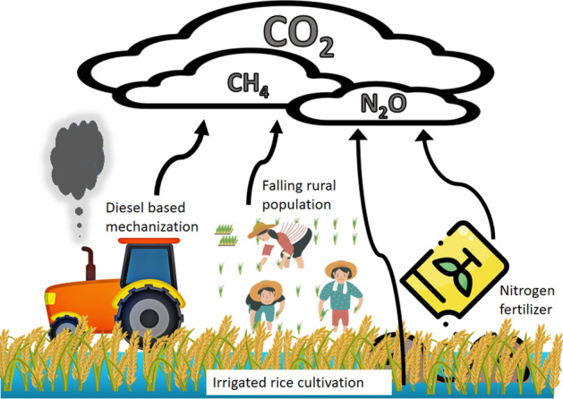
Graphic abstract

Introduction

A historic event occurred in Bangladesh in 2014, when for the first time in modern history, the rural population of the country peaked and then started to decline (World Bank, 2020) (Fig. 1, 2, 3). In 2020, Bangladesh also became the third biggest rice producing nation, after China and India. In order to support the growing population, the government emphasized increasing the production and yield in the agriculture sector, and as a result, the yield of the land has almost doubled during this period, though the area of cultivated land increased little (Figs. 4, 5) (World Bank, 2020). Following a great flood in 1988, the government took widespread measures to stimulate the agriculture sector, but this came at the expense of environmental degradation and pollution. It instilled policies to subsidize diesel, as well as agricultural machinery, and allowed tax free imports of the machinery, all of which expanded their sales. It also removed restrictions on boring and groundwater extraction, leading to uncontrolled groundwater pumping. The shortage of rural labor during brief and busy harvesting periods, and a local industry for manufacturing agricultural machinery, have further increased dependence on mechanization (International Development Enterprise, 2012). Food security is also a motivation for mechanization, as the machines reduce crop damage and wastage, and enable quick harvests during emergencies before anticipated climate disasters (International Development Enterprise, 2012).

Fig. 1.

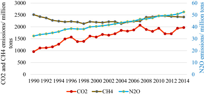
Trend of GHGs from agriculture

Fig. 2.

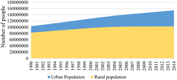
Population trend in Bangladesh

Fig. 3.

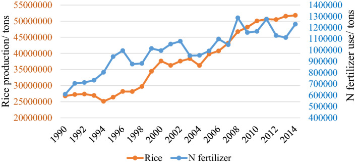
Rice production and fertilizer use trends in Bangladesh

Fig. 4.

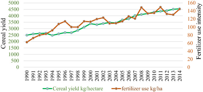
Cereal yield and fertilizer use intensity trends in Bangladesh

Fig. 5.

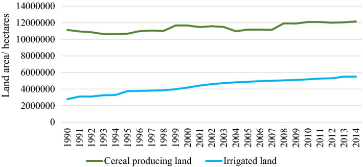
Growth of cereal producing land area and irrigated land area in Bangladesh

However, the mechanization and irrigation intensity of agriculture makes it one of the most energy consuming sectors in the country. The agriculture sector of Bangladesh is second in petroleum consumption (19%), after the transport sector (45%) (SREDA & MoPEMR, 2015). To mitigate this, there is government initiative under the Ministry of Agriculture and the Ministry of Power, Energy and Mineral Resources to introduce renewable energy based irrigation on a massive scale, by using solar irrigation (SREDA & MoPEMR, 2015). Despite this, the falling rural population is leading to greater mechanization in all stages of agriculture, including tilling, planting and harvesting. In the past, agriculture subsidies from the government were allocated to farmer credit, seeds, fertilizers and pesticides (BBS, 2020). Now, the worldwide lockdowns due to Covid-19 in 2020 have led the government to reemphasize the importance of food security, in a world where trade flows may become obstructed. Therefore, the new budget has increased subsidies for agricultural machinery as well (Bhuyan, 2020).

The lack of widespread use of expensive farm machinery in the past was due to the ample availability of rural labor, lack of capital and small size of land holdings. The decreasing rural population (Fig. 2) and the potential productivity increase from mechanization has now created a large untapped opportunity for mechanization (Alam et al., 2020; Fuad & Flora, 2019). Bangladesh already has a roadmap for the achievement of the Nationally Determined Contribution (NDC) target of reducing greenhouse gases (GHG) emissions from the power, industry, transport and agriculture sectors. The aim is to reduce emissions by 5% unilaterally, or by 15% with international support, by 2030. This roadmap expressly aims to reduce methane emissions from agricultural land. The plan also aims to reduce the overall energy intensity of the economy by 20% within 2030 (MOFE, 2015).

Urbanization and a declining share of rural population is a feature of developing countries across the world, and especially the largest agriculture producing developing countries like China, India, Indonesia and Bangladesh. However, to our knowledge, the impacts on agricultural emissions from a falling share of rural population, alongside the changing technology and land use patterns have not been studied.

Rice cultivation, starting in historic times over 5000 years ago, has been a top emissions source of CH₄, but the process has been accelerating in recent years and decades, with the increase in the populations and economies of the top rice producers of the world, the populous Asian countries (Li et al., 2009). Agriculture also represents the biggest source of anthropogenic N₂O emissions, due to the application of artificial nitrogen-rich fertilizers, soil management practices and biomass management (Reay et al., 2012). In addition to CO₂, CH₄ and N₂O make up the second and third largest share of greenhouse gases (16% and 6% respectively). Furthermore, agriculture, forestry and land use emit 24% of the GHGs worldwide (EPA, 2020). Rosa et al. (2004) studied the anthropogenic drivers of GHGs across countries, and Singh and Mukherjee (2018) studied GHG emissions from livestock farming in America. However, to our knowledge, there has been no study of the socioeconomic drivers of specifically methane (CH₄) and nitrous oxide (N₂O) emissions from the agriculture sector.

The emissions of CO₂ depend on the use of fossil fuel-based energy for irrigation, tillage and cultivation, and the energy intensity of the process. Among anthropogenic sources, rice agriculture plays as great a role in CH₄ emissions as energy consumption, and agricultural soil management activities are responsible for more N₂O emissions than any other source (Inamori et al., 2003; Scheehle & Kruger, 2006). Among SAARC countries, Bangladesh has a middle rank when it comes to CO₂ emissions from agriculture, coming after Pakistan and India, but above Afghanistan and Bhutan (Ikram et al., 2020). Bangladesh also has the lowest CO₂ emissions intensity from rice production among top eight rice producing countries (Maraseni et al., 2018). However, the overall emissions show an increasing trend. Studies of the drivers of greenhouse gases in the electricity sector in Bangladesh have shown that energy intensity, carbon intensity, population, affluence and urbanization all play important roles (Aziz & Chowdhury, 2020). The effects with respect to the agriculture sector have not been previously explored.

In the context of the demographic and energy transition in Bangladesh, the aim of this study is to analyze impacts of population, rural population change, affluence, urbanization, and selected energy and agricultural technologies on the emissions caused by the agriculture sector in the Bangladeshi economy. Using the STIRPAT model and ridge regression, in this study we hope to add to the literature by exploring the anthropogenic sources of the three salient atmospheric emissions of agriculture, CO₂, N₂O and CH_4, in the context of Bangladesh. We investigate the effects of some new factors previously not explored for the agriculture sector, namely the linear and nonlinear effects of rural population, the linear and nonlinear effects of urbanization, land area under grain cultivation, irrigated land area, rice cultivation quantity and the land yield. We show their implications for achieving the climate targets of the country, alongside the socioeconomic goals. The findings from Bangladesh will also shed light on the effects of the socioeconomic drivers of GHG emissions from agriculture in other major rice growing countries, which are also undergoing some of the same demographic and energy transitions.

With respect to the emission of CO₂, we test the following hypotheses:

1. The carbon intensity of agriculture increases CO₂ emissions.

2. The energy intensity of agriculture increases CO₂ emissions.

3. Urbanization trends increase CO₂ emissions.

With respect to the emissions of CH₄, we explore the following hypotheses:

1. Higher crop yield increases the emissions of CH₄

2. More rice cultivation increases the emissions of CH₄

3. Greater irrigated land area increases the emissions of CH₄

4. Greater cultivated land area increases the emissions of CH₄.

With respect to N₂O emissions, we explore the following hypotheses.

1. Higher fertilizer intensity increases N₂O emissions.

2. Greater fertilizer use increases N₂O emissions.

Furthermore, we also explore the effects of rural population decline, and its nonlinear effects, on the emissions of all three gases. Overall country population and affluence are used as control variables.

The factors affecting emissions can vary depending on the specific GHG, and can include drivers like energy intensity, carbon intensity, land use, fertilizer use, irrigation patterns and crop yields. Drivers like population and affluence are common factors in increasing the emissions of all GHGs. However, energy use is primarily responsible for CO₂ emissions, irrigation and rice production increases CH₄ emissions, and fertilizer use affects N₂O emissions. The studies exploring the drivers of the three GHGs in our literature review are summarized in Table 1.

Table 1.

Review of literature on drivers of GHG emissions from agriculture

Research	Country/location	Greenhouse gas emissions	Findings
Cui et al. (2018)	Hebei province, China	Carbon emissions	Affluence, urbanization, agricultural population and mechanization increase carbon emissions
Long et al. (2018)	China	Carbon intensity	Population, GDP and urbanization have positive impacts
Li et al. (2014)	China	CO2 emissions	Population and affluence increase emissions
Parajuli et al. (2019)	86 countries of different regions	CO2 emissions	Increase in agricultural land increases CO2 emissions
Lin and Xu (2018)	Provinces of China	Agricultural CO2 emissions	Population, GDP and urbanization have a positive effect, and energy efficiency has a negative effect
Xu and Lin (2017)	Provinces of China	Agricultural CO2 emissions	Population, GDP, energy intensity and urbanization have a positive effect
Hamilton and Turton (2002)	OECD countries	CO2 emissions	Energy intensity of agriculture increases CO2 emissions
Yan et al. (2017)	Selected European countries	GHG emissions	Energy intensity and carbon intensity increase emissions of GHGs
Maraseni et al. (2009)	Selected developing and developed countries	GHG emissions	Crop yield, mechanized irrigation and chemical fertilizer use increase emissions
West and Marland (2003)	Land samples	CO2 emissions	Increased crop yield and decreased land use can reduce emissions
Minami and Neue (1994)	Land samples	Methane emissions	Irrigation intensity affects methane emissions
Smith (2005)	Land samples	N2O emissions	Use of fertilizer can affect N2O emissions positively
Bhatia et al. (2013)	India	Methane emissions	Rice cultivation increases methane emissions
Neumann et al. (2014)	Bangladesh	Methane emissions	Groundwater irrigation can increase methane emissions
Johnson, Franzluebbers, Weyers, & Reicosky (2007)	Land samples	N2O emissions	Fertilizer choice and intensity increase N2O emissions
Selden and Song (1994)	OECD countries	Different GHGs	Population density has nonlinear effects on emissions
Lantz and Feng (2006)	Canada	CO2 emissions	Population has a nonlinear effect on CO2 emissions
Ali et al. (2017)	Pakistan	CO2 emissions	Fertilizer use and production of tractors affect CO2 emissions
Abbas, et al. (2020)	Pakistan	CO2 emissions	Total population increases emissions, rural population and agricultural land have an insignificant impact

Increasing agricultural production itself leads to increase of CO₂ emissions, though using clean or renewable energy in agriculture can reduce these emissions (Anwar et al., 2019; Aziz et al., 2020; Liu et al., 2017; Waheed et al., 2018).

The nonlinear effects of anthropogenic drivers have also been studied in the STIRPAT literature, most commonly the affluence driver. This is in the framework of the environmental Kuznets curve (EKC) hypothesis, which was pioneered by the research of Shafik and Bandyopadhyay (1992) and Grossman and Krueger (1991). It proposes that low income countries pollute the environment in the course of economic activities, but after reaching a certain level of affluence, invest in clean technologies and policies to reduce pollution. This relationship is captured by an inverted U-shaped curve created by the environmental degradation variable as a function of income. The nonlinear effects of population on overall country emissions have been studied by Selden and Song (1994) and Lantz and Feng (2006). However, we have not found studies which explore the nonlinear effects of urbanization or population, or rural population in particular, on the agriculture sector in particular, and hope to address this gap in our research.

Using our literature survey as a guide, we explore the impact of critical anthropogenic factors affecting emissions of the top three GHGs from the agriculture sector of Bangladesh. We prepare separate models for each of the gases, including the factors most indicated to influence their emissions. We will also explore the nonlinear effects of rural population and urbanization on emissions, as the total rural population of the country has turned a corner, and begun to decrease.

Methodology

Analytical model

The literature exploring the factors behind atmospheric emissions includes a number of socioeconomic, demographic and technological factors, often summarized in the STIRPAT (Stochastic Impacts by Regression on Population, Affluence, and Technology) model, proposed by Dietz and Rosa (1994). This model has been used to reveal the causes of emissions in a number of sectors, countries or groups of countries. These studies reveal that the factors responsible for increasing emissions include rising population, increasing affluence, urbanization, economic structure, energy consumption, energy mix and related technological aspects of the country. We use this STIRPAT model in our research. The STIRPAT model is derived from an earlier IPAT model developed by Ehrlich and Holdren (1971). The basic IPAT model can be stated as

$$I=P\ast A\ast T,$$ 1

where P is the population, A is the affluence, and T is the technology term. They together form a multiplicative relationship to affect the dependent variable I. This variable I indicates the environmental impact, which can be a measure of pollution, like greenhouse gas emissions. The initial multiplicative specification of the model implies that the relationship among the driving forces is not independent of one another, and changes in one factor are multiplied by the other factors. No one factor is alone responsible for the environmental impacts. The drivers create impacts at different scales and different rates. However, a limitation of the multiplicative form is that it assumes there is a proportional relationship among the explanatory variables, which may not be empirically founded. This multiplicative form also did not allow the type of analysis needed for hypothesis testing or the assumption of nonlinear effects. To overcome this, Dietz and Rosa proposed an additive form of the model, by taking the logarithms of the terms and converting it into a regression model, in the following steps:

$$I_i=a{P}_i^b{A}_i^c{T}_i^d{e}_i$$ 2

In the first step, $I_i$ is the impact in observational unit i from population P, affluence A and technology T. This equation is multiplicative, but converting the terms into their logarithms makes it additive, as follows

$$\ln I=a+b(\ln P)+c(\ln A)+\mathrm{d}(\ln T)+e$$ 3

York et al., (2003) further demonstrated the use of the model to account for the technology term, which can include one or more factors according to the needs of the research. The coefficients of the variables can be interpreted as ecological elasticities, where the coefficient represents the percentage change in the impact variable for one percentage change in the explanatory variable. The STIRPAT model allows the principle of model parsimony to be met, as a limited number of significant variables account for a high degree of the variance in the environmental impact dependent variable.

We prepare three STIRPAT models for the three gases as follows.

$$\ln I_{{\mathit{CO}}_2}=a+b_1(\ln P)+b_2\left(\ln ,R,P\right)+b_3\left(\ln ,R,P,2\right)+b_4\left(\ln ,A\right)+b_5\left(\ln ,U\right)+b_6\left(\ln ,U,2\right)+b_7\left(\ln ,E,I\right)+b_8\left(\ln ,C,I\right)+e$$ 4

$$\ln I_{{\mathit{CH}}_4}=a+b_1(\ln P)+b_2\left(\ln ,R,P\right)+b_3\left(\ln ,R,P,2\right)+b_4\left(\ln ,A\right)+b_5\left(\ln ,C,Y\right)+b_6\left(\ln ,L,A\right)+b_7\left(\ln ,L,I\right)+b_8\left(\ln ,R,C\right)+e$$ 5

$$\ln I_{N_{2}O}=a+b_1(\ln P)+b_2\left(\ln ,R,P\right)+b_3\left(\ln ,R,P,2\right)+b_4\left(\ln ,A\right)+b_5\left(\ln ,U\right)+b_6\left(\ln ,U,2\right)+b_7\left(\ln ,F,I\right)+b_8\left(\ln ,F\right)+e$$ 6

A comprehensive review of 112 STIRPAT-based studies by Vélez-Henao et al. (2019) revealed that there is often multicollinearity among the explanatory variables, and a common solution to this in the literature is to apply ridge regression. In this analysis, we will use as measures of technology the energy intensity, carbon intensity, fertilizer use, fertilizer intensity, land area under cultivation, irrigated land, rice cultivation and agriculture yield of the land. We will also apply ridge regression, after testing for multicollinearity.

Variables

The dependent variables used in this study are the CO₂, CH₄ and N₂O emissions from agriculture. The population variables are the population of Bangladesh in each of the studied years, and the rural population. The total population represents the number of people dependent on the agricultural output. The rural population on the other hand indicates how many people work in the agriculture sector. We have included the quadratic term for the rural population to investigate the nonlinear effects. Urbanization is the share of the population living in urban areas, and the quadratic term is to detect nonlinear effects. A decrease in the rural population leads to an increased dependence on mechanization. The affluence variable is the real GDP per capital. The carbon intensity of energy indicates to what extent clean energy is used in the irrigation and overall mechanization of agriculture process. The energy intensity is a proxy for artificial irrigation using diesel pumps and the use of agricultural machinery in case of CO₂ emissions. In the model for the CH₄ emissions, we will also include the area of land under cultivation, area of land under irrigation, amount of rice cultivated and the crop yield of the land. In the N₂O model, we include the quantity of nitrogen fertilizer use, and the intensity of nitrogen fertilizer. The GDP per capita and the net operating surplus of agriculture used to calculate emission intensity are expressed in constant USD with base year 1990. Table 2 displays the variables and their details. Figures 1,2,3,4 and 5 show the trends of the variables. The N₂O and CH₄ emissions are the direct and indirect emissions from agriculture in thousand tons.

Table 2.

Variables used in the model

Dependent variable	Description	Unit
CO2_emissions	Carbon dioxide emissions from agriculture	Thousand tons
CH4_emissions	Methane emissions from agriculture	Thousand tons
N2O_emissions	Nitrous Oxide emissions from agriculture	Thousand tons
Independent variables
Population (P)	Population size of the country	Number of persons
Rural population (RP)	Number of rural inhabitants	Number of persons
Rural population square (RP2)	Square of rural population to capture nonlinear effects
Urbanization (U)	Urban population as percentage of total population	Percentage
Urbanization square (U2)	Square of urbanization to capture nonlinear effects
GDP per capita (A)	GDP per capita in real USD	USD
Energy intensity (EI)	Energy used per unit of industry income	Ktoe/ million USD
Carbon intensity (CI)	Emissions per unit of fuel used	Thousand tons/ktoe
Fertilizer use (F)	Amount of nitrogen-based fertilizer used	Tons
Cereal yield (CY)	Quantity of grain produced per unit land area	Kg/hectare
Land area (LA)	Area of land under agricultural cultivation	Hectare
Land irrigated (LI)	Area of lander under irrigation	Hectare
Rice cultivated (RC)	Amount of rice cultivated	Million tons
Fertilizer use intensity (FI)	Amount of nitrogen fertilizer used per land area	Kg/hectare

Data and study period

We have analyzed data from 1990 to 2014, covering a period of 25 years. This time period is chosen because the government stimulus to increase mechanization, fuel consumption and artificial irrigation in agriculture started at the beginning of this period, and in 2014, the rural population peaked, while in 2015, Bangladesh committed to NDC targets. The data for the production of the agriculture sector are obtained from the Eora multiregional input output (MRIO) tables created by Lenzen et al., (2013). As this is an environmentally extended input output database which disaggregates economic value addition at the sectoral level, we found this to be the best option to isolate the effects of the agriculture sector exclusively. This is also the only input output database to our knowledge which includes data for more than 180 countries including Bangladesh, covering several decades. The data for energy consumption in the sector are obtained from International Energy Agency (IEA) (IEA, 2020), and the CO₂ emissions data area obtained from PRIMAP (Gütschow et al., 2016, 2019). The energy intensity and carbon intensity are calculated from the data here. The data for the population, rural population, urbanization rates, GDP per capita, cereal yield and land under cereal cultivation are obtained from the World Bank country database for Bangladesh (World Bank, 2020). The monetary data for GDP per capita, and the net operating surplus for the sector used to calculate the energy intensity of that sector, are originally available in current USD, but are converted to constant USD taking 1990 as the base year. The data for the CH₄ and N₂O emissions are taken from the Emissions Database for Global Atmospheric Research (EDGAR) database. Here, the total (direct and indirect) N₂O emissions from managed soils are used, and the CH₄ emissions from agriculture and rice cultivation are used (EDGAR, 2020). The values for nitrogen fertilizer use in agriculture, nitrogen fertilizer intensity, rice cultivated and land area under irrigation were obtained from the Food and Agriculture Organization database (FAOSTAT, 2020).

Ridge regression analysis

Ridge regression is used to solve the issue of multicollinearity that has been revealed from the VIF values of the ordinary least squares (OLS) regression analysis. It is a biased estimation method that is effective for creating models with improved overall predictive ability and for reducing multicollinearity. The method was originally developed by Hoerl and Kennard (1970), and has been shown to have better predictive abilities by introducing a small amount of bias in the model, which will reduce the overall variance and avoid over fitting. This property makes it suited to estimating STIRPAT models, especially because the STIRPAT explanatory variables often have multicollinearity among themselves. In ordinary least squares, we estimate the coefficients using the following formula in matrix form:

$$\widehat{\beta }={\left(X{X}^{\prime }\right)}^{-1}\left(X{Y}^{\prime }\right)$$ 7

The ridge regression formula is a modification of this by adding a positive quantity lambda, λ, which is the ridge coefficient, a biasing parameter, with values between 0 and ∞:

$$\widehat{\beta }={\left(X{X}^{\prime }+\mathrm{\lambda }I\right)}^{-1}\left(X{Y}^{\prime }\right)$$ 8

When λ has a value of 0, ridge regression gives the same results as OLS. For estimating ridge regression, the values of λ should ideally be between 0 and 1. As per the requirements of the STIRPAT methodology, the original data are first converted into logarithmic form, and an OLS analysis is performed to check for multicollinearity. The variance inflation factors (VIF) of the independent variables are checked. Finally, ridge regression analysis is done to find out the coefficients of the explanatory variables.

The proper values of λ are found by trying values starting from 0.01 with increments of 0.01, until the VIF values of all the independent variables go below 10 and coefficients stabilize. This estimation method has been shown to perform well when the sample size is limited, the number of explanatory variables is many compared to the sample size, and when there is multicollinearity (Kibria, 2003). It has been often used for similar studies for the agriculture sector (Cui et al., 2018), for countries and locations (Lin et al., 2009; Wang et al., 2013), for water footprint analysis (Zhao et al., 2014) and others included in a review by Vélez-Henao et al (2019). We have used Excel, SPSS 16 and Eviews 9 software to conduct the OLS and ridge regression analyses.

Results

The preliminary test for multicollinearity in our variables using OLS regression has revealed that the independent variables in all cases have very high VIF values. This shows high multicollinearity (Table 3). Furthermore, the signs of some of the variables, like crop yield, land area and urbanization, are at times negative, which does not reflect their theoretical validity. The coefficients of variables like population, rural population, affluence, fertilizer and urbanization are not always statistically significant. All this indicates that the OLS results would lead to conclusions which are contrary to the theoretical validity of the relationships among the variables (Kidwell & Brown, 1982).

Table 3.

OLS results for the three STIRPAT models

Variable	Coefficients	t-statistic	Sig	VIF
	OLS regression results for CO2
LnP	2.302	0.628	0.538	13,804.648
LnRP	0.385	0.454	0.655	92.441
LnRP2	−69.149	−2.746	0.013	904,837.3
LnA	0.569	2.639	0.016	29.548
LnU	−1.396	−0.165	0.871	72,129.48
LnU2	0.158	2.083	0.051	162.753
LnEI	0.487	4.021	0.001	35.241
LnCI	0.752	6.509	0.000	29.837
Constant	−6.375	−0.414	0.683
R2	0.982
F-statistic	208.55
P value	0.0000
	OLS regression results for CH4
LnP	0.613	1.947	0.068	447.812
LnRP	−1.471	−3.919	0.001	209.797
LnRP2	86.481	1.378	0.187	3,120,202
LnA	0.119	1.766	0.095	33.844
LnCY	−1.962	−5.773	0.000	1503.505
LnLI	−0.057	−0.613	0.548	102.299
LnLA	−1.101	−3.974	0.001	43.051
LnRC	1.958	6.644	0.000	1589.123
Constant	49.735	7.041	0.000
R2	0.977
F-statistic	105.027
P value	0.0000
	OLS regression results for N2O
LnP	2.416	1.295	0.212	15,874.43
LnRP	77.236	2.568	0.019	5,155,133
LnRP2	0.011	2.696	0.014	26.799
LnA	0.038	0.509	0.616	31.231
LnU	−4.003	−0.968	0.346	75,083.12
LnU2	0.082	4.939	0.000	69.886
LnFI	0.167	1.499	0.150	136.834
LnF	−0.075	−0.617	0.545	126.237
Constant	−0.911	−0.420	0.679
R2	0.996
F-statistic	876.75
P value	0.000

In order to account for this multicollinearity, we have employed ridge regression for each model. The values of λ for which the VIF values fall below 10, and the resultant ridge regression coefficients for each of the gases are shown in Table 4. Figures 6, 7 and 8 show the ridge trace graphs for the three models. We can see that the values of the coefficients of the variables start to stabilize as the values of λ increase. After trials of incremental values of λ, at λ values of 0.03, 0.06 and 0.09, we find that the VIF values are all below 10, and the coefficients are also stable, for the three GHGs respectively, as given in Table 3. The R² of the models have high values, and the F statistics are statistically significant. The coefficients of the variables in the three models are also statistically significant.

Table 4.

Ridge regression results for the three STIRPAT models

Variable	Coefficients	t-statistic	Sig	VIF
	Ridge regression results for CO2
LnP	0.332235	4.649918	0.000229	0.612114
LnRP	0.833081	4.64322	0.000233	1.274994
LnRP2	0.022491	4.624193	0.000242	1.262623
LnA	0.39931	2.542791	0.021019	4.848716
LnU	0.13822	1.78508	0.092102	1.235411
LnU2	0.019243	1.475465	0.158369	1.479082
LnEI	0.192419	2.5758	0.019638	4.138086
LnCI	0.418596	5.272666	0.000065	4.354048
Constant	−25.7
R2	0.948
λ	0.03
F-statistic	38.9
P value	0.00000
	Ridge regression results for CH4
LnP	−0.06356	−1.85812	0.080557	0.671981
LnRP	−0.34947	−6.34878	0.000007	0.574856
LnRP2	−0.00943	−6.32021	0.000007	0.569141
LnA	0.198794	4.327977	0.000457	1.987107
LnCY	0.066399	2.179417	0.043654	1.538568
LnLI	−0.07391	−2.29685	0.034604	1.583335
LnLA	0.527602	3.077357	0.006828	2.100351
LnRC	0.087844	3.656672	0.001953	1.344805
Constant	8.35639
R2	0.8225
λ	0.06
F-statistic	9.45
P value	0.0000
	Ridge regression results for N2O
LnP	0.169181	10.33008	0.000000	0.199135
LnRP	0.213627	4.314947	0.00047	0.601112
LnRP2	0.005814	4.306842	0.000478	0.602293
LnA	0.135208	4.186774	0.000619	1.269688
LnU	0.14876	8.431696	0.000000	0.39715
LnU2	0.023322	7.912239	0.000000	0.467809
LnFI	0.052763	2.539832	0.021147	1.013752
LnF	0.052519	2.143876	0.046796	1.075298
Constant	−7.95157
R2	0.981819
λ	0.09
F-statistic	114.7553
P value	0.00000

Fig. 6.

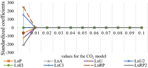
Ridge trace graph of standardized coefficients against λ values for CO₂

Fig. 7.

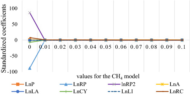
Ridge trace graph of standardized coefficients against λ values for CH₄

Fig. 8.

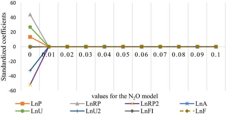
Ridge trace graph of standardized coefficients against λ values for N₂O

Discussion

With respect to CO₂ emissions, our results show that the biggest factor is the rural population, followed by carbon intensity, affluence, population, energy intensity and urbanization. An increasing population is responsible for emissions, as the rise in the number of consumers of rice and other agricultural products in itself leads to increasing use of energy for cultivation. The findings for the effects of total population on CO₂ emissions reflect those of Abbas et al. (2020) for Pakistan, and Long et al. (2018) and Li et al. (2014) for China. However, there is a much stronger relationship between the rural population and CO₂ emissions. The rural population in our CO₂ model has the biggest coefficient, with a value of 0.83, and is statistically significant. Although the staple foods of rural and urban people are alike, rural populations use the agricultural biomass as a source of fuel, and this leads to significant amounts of emissions. These findings on the effects of rural population correspond to those of Cui et al. (2018) for China. However, the quadratic term for the rural population is positive, showing that the effect is linear. It implies that as the rural population falls further in the future, the emissions of CO₂ can slow down in the long run. Although nonlinear effects of rural population have not been found in the literature, Selden and Song (1994) found population density to have nonlinear effects in OECD countries, and Lantz and Feng (2006) have found nonlinear effects of population in Canada. Or results for nonlinear effects of rural population in Bangladesh diverge from these findings in the case of high income countries.

The results for urbanization rate show that the greater the share of urban people in the population, the more are the emissions from this sector. The urbanization rate has no evidence of a nonlinear effect either, as the coefficient of the quadratic term of urbanization has a positive sign. This indicates that at the present time, increasing rates of urbanization beyond a certain level will not result in decreasing emissions of agricultural CO₂. These findings on the effects of urbanization are similar to those of Cui et al. (2018), Long et al. (2018), Lin and Xu (2018) and Xu and Lin (2017) for China. The affluence of the population has a major impact on CO₂ emissions, as people consume more agricultural products with an increase in purchasing power.1 This too corresponds to the findings of Cui et al. (2018), Long et al. (2018), Lin and Xu (2018) and Xu and Lin (2017) for China. The energy intensity of agriculture has a prominent impact on emissions, indicating that as the sector becomes more mechanized, there is greater consumption of fossil fuels, leading to more emissions. This confirms that the migration of people from the countryside to the cities over the last few decades has resulted in increasing dependence on agricultural mechanization, with accompanying emissions. Moreover, the carbon intensity of the fuels in the energy mix also has a strong impact. This is because a chief fuel used in farming machinery is diesel, which is relatively more polluting than natural gas or grid electricity. The increasing rate of mechanization leads to a greater share of carbon intensive fuels in the energy mix of the sector. Our findings on the positive effects of energy intensity and carbon intensity on emissions reflect those of Hamilton and Turton (2002) for OECD countries, Yan et al. (2017) for European countries, and Maraseni et al. (2009) for some developed and developing countries.

In the case of CH₄ emissions, the biggest impact comes from the land used for agriculture of grains. A 1% increase in the land dedicated to rice cultivation contributes to 0.53% increase in CH₄ emissions. Our findings on the effects of land use reflect that of Parajuli et al. (2019). This stresses the importance of land management in the country. However, the coefficient for irrigated land area has a negative value, indicating that the more the area of land under artificial irrigation, the lower the CH₄ emissions. Although soil flooding is supposed to increase CH₄ emissions, in the context of Bangladesh, increasing artificial irrigation implies increasing the number of harvests per year. This is because artificial irrigation is required for one or two out of the three harvests per year, depending on the location. When there are more harvests, there is automatically more tilling of the soil, leading to decreased anaerobic conditions, and lower CH₄ emissions. These findings on the effects of irrigation on CH₄ emissions add to those of Neumann et al. (2014) and Minami and Neue (1994).

Increasing affluence of the population leads to increasing CH₄ emissions, as there is more demand on rice and agricultural production. The total population increase on the contrary has a negative impact on CH₄ emissions. A rising population leads to a more intensive cultivation of a limited area of land, which can lead to more frequent tilling and therefore more aerobic conditions in the soil. Moreover, the demands of feeding a bigger population have led to the cultivation of high yield varieties of rice and other crops, which results is lower emissions relative to the quantity of crops produced. This corresponds to the findings of Bhatia et al. (2013). However, the rural population has a large negative impact on CH₄ emissions. The falling rural population has led to increasing CH₄ emissions. Rural inhabitants use agricultural biomass as thatching material or fuel, and a decline in rural populations may lead to the anaerobic decomposition of residual biomass in fields, which are sources of CH₄ (Karakurt et al., 2012). The quadratic term for the rural population has a negative sign, indicating a nonlinear relationship. This implies that as the rural population further decreases, CH₄ emissions are expected to increase at a slower rate. This can be due to the inclusion of technology which reduces CH₄ emissions. The crop yield of the land has a positive effect on CH₄ emissions. In order to increase yield and obtain three harvests per year, agricultural land is artificially irrigated throughout the year, leading to soil conditions that generate CH₄. Rice cultivation has a positive impact on CH₄ emissions, as it is dependent on irrigation, and this is predicted by previous research of Li et al. (2009). However, our research also reflects that of Maraseni et al. (2018), in that the coefficient of rice cultivation is actually much lower than that of some of the other variables.

In the emissions of N₂O, the total population and the rural population have the highest impact. This is a positive impact, as increase in population leads to increase in use of nitrogen fertilizer to increase yield. Unlike in the case of CH₄, there is no negative relationship with the rural population. N₂O emissions are related to mainly fertilizer use. The relationship is also linear, which indicates that as the rural population declines over the years, emissions should drop in the long run. Affluence has an impact on N₂O emission, as greater agricultural demand arises from higher purchasing power spurring more cultivation. The impact of urbanization is also positive and linear. As there is more urbanization, there is greater demand for agricultural supplies to the cities. Nitrogen fertilizer use and fertilizer intensity both have positive impacts, reflecting earlier findings of Smith (2005) and Johnson et al. (2007). This arises out of residual fertilizer in the soil, not absorbed by the crops. Fertilizer use in excessive amounts can lead to higher emissions of N₂O, and our results indicate that agriculture in Bangladesh applies fertilizer in excessive quantities.

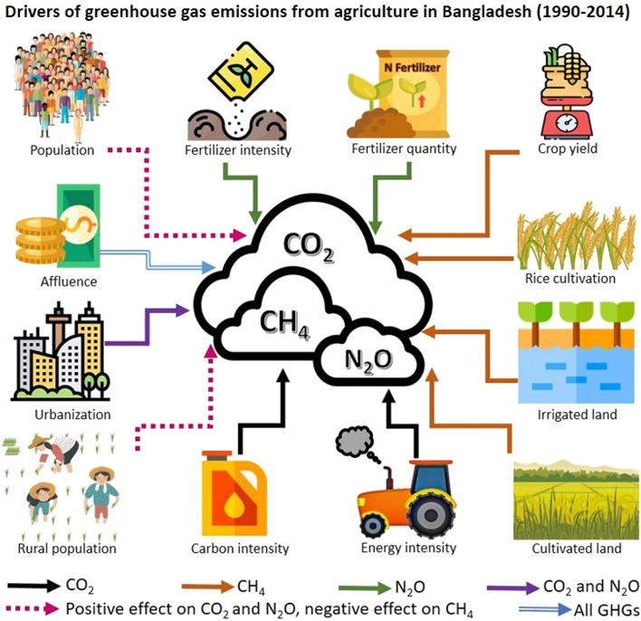
Our results reflect the findings of Maraseni et al. (2009), who found that developing countries are less successful in controlling agricultural emissions. However, they are contrary to the findings indicated by Ali et al. (2017) that although the long-term CO₂ emissions are affected by fertilizer use in Pakistan, irrigated land or land yield does not. Figure 9 summarizes the findings of the analysis.

Fig. 9.

Patterns of factors affecting emissions of the three GHGs

In Bangladesh, the diesel run irrigation system is switching to grid electricity, and there is the dissemination of solar irrigation units around the country. However, the progress in this sector is very slow. There are at present 1.34 million diesel irrigation pumps in the country, and the current plan is to replace only one third of them with solar pumps over the next fifteen years (Ahmed, 2019). Furthermore, the mitigation effects of the solar irrigation can be offset by the increase of farm machinery and vehicles. However, the use of solar irrigation pumps is supposed to reduce the use of water by up to 50%, due to the lack of evaporation loss, and the loss into non-agricultural layers of the soil (Hasan, 2019). The total number of shallow diesel pumps increased from around 200,000 to around 1.5 million from 1990 to 2014, accounting for 73% of groundwater irrigation, covering 53% of the total irrigated land. Seventy-eight percent of the equipment uses diesel, and most of the remaining run on electricity, although since 2014, the number of these pumps has decreased (MOA, 2018). The roadmap for NDC implementation states the plan to increase the number of solar irrigation pumps, but it is expected that most of the diesel based pumps will switch to electricity in the electrified areas (MoEFCC, 2018).

In addition to irrigation equipment, Bangladesh has seen an increase of 500,000 two-wheel tractors, and the market for four-wheel tractors, rice threshers and rototillers is also increasing through the expansion of agricultural services marketing and credit purchase options. These machineries run on diesel, and there is no clear plan to incorporate clean energy into this part of the agriculture production process (International Development Enterprise, 2012).

Considering the energy use and agricultural practices in Bangladesh, the government must step up the drive to reduce emissions to attain climate targets. At present, there are more than 1700 solar irrigation pumps in Bangladesh, and IDCOL (Infrastructure Development Company Limited), the financial institution responsible for their dissemination, has plans to increase the number to 50,000 by 2025, substituting more than 300,000 diesel pumps (Jude et al., 2019). This must in addition be accompanied by policies to control the amount of irrigation and other soil management practices to combat emissions of CH4 and N₂O. The alternate wetting and drying (AWD) method of irrigation should be introduced and enforced among farmers, which has the potential to reduce the emissions of these two gases by 24% in the rice fields of Bangladesh (Begum et al., 2019). Another estimate by Islam et al. (2020) in Bangladesh also shows that AWD results in a net reduction in greenhouse gas emissions by 36% from the soil of rice fields, compared to continuous flooding, without loss of yield. There is also a great scope for reducing the emissions by increasing the share of renewable energy through the use of solar irrigation, according to Liu et al. (2017), Aziz et al. (2020) and Naseem and Ji (2020). Therefore, there should be the formulation and implementation of energy efficiency and fuel quality standards in agricultural machinery, and the implementation of water conserving irrigation methods. The objectives of crop yield maximization and renewable energy incorporation can be realized through innovative solutions like agrivoltaics, which uses solar panels installed in crop land to generate renewable electricity.

Conclusion and policy recommendations

In this study, we have used an extended STIRPAT model to explore the relationship of demographic, socioeconomic and technological factors on the emissions of three top greenhouse gases, CO₂, CH₄ and N₂O, from the agriculture sector in Bangladesh. We have used ridge regression to estimate the model, for a twenty-five year period covering 1990 to 2014. Our findings indicate that the emissions of the three greenhouse gases will keep increasing, given the trends in the driving factors. Unless steps are taken to curb or mitigate the drivers, this will have negative implications on meeting the clean energy and climate targets of the country.

The population of Bangladesh is stabilizing, as the country fertility rate has been brought under control, having fallen from 6.9 in 1971 to 2.05 births per woman in 2020 (United Nations, 2021; World Bank, 2020).

However, urbanization, the migration of the rural population, and the increase in affluence are continuing trends, and places demand on agricultural productivity. In order for Bangladesh to meet the clean energy and climate change mitigation goals, it must take urgent measures to implement emission reducing technologies in the agricultural sector. Some measures that can prove effective include increasing the number of solar irrigation pumps, incorporate renewable energy into agricultural vehicles and machinery, and implementing the alternate wetting and drying method of irrigation.

Finally, the issue of GHG emissions cannot be tackled from the policy guidelines covering energy alone. Although the NDC plan (MOFE, 2015) and the Energy Efficiency and Conservation Master Plan up to 2030 (SREDA & MoPEMR, 2015) recognize the need of reducing emissions, they largely focus on the energy side of it. The NDC plan proposes ways to reduce CH₄ from agriculture, but no plans for N₂O. The same is true for the Bangladesh Delta Plan 2100 (GED, 2019). The National Water Management Plan (MoWR, 2001) does not mention emissions or GHGs, and discusses environmental concerns in terms of aquatic ecosystem conservation. The same is true for the National Land Use Policy (GOB, 2016), which discusses environmental degradation and ecosystem preservation, without reference to GHG emissions. The prevention of emissions of all significant GHGs should be elaborated in the land use policy, water use policy and long-term climate adaptation plans as well, to maintain coordinated and effective efforts.

A limitation of this study is that the effects of natural and artificial irrigation could not be separated due to lack of data. Year wise data for the stock of machinery were also not available. Future scope for research could be the measurement of volume of groundwater pumped for irrigation and the quantity of fuel used in agricultural machinery and vehicles. This would enable a more disaggregated study of effects and more specific policy recommendations.

Funding

Funded by Institute for Advanced Research publication grant reference no. IAR/2022/Pub/011, of United International University.

Declarations

Conflict of interest

The authors declare that they have no conflict of interest.

Availability of data and material

Data are obtained from freely and publicly available data sources.

References

- Abbas S, Kousar S, Yaseen M, Mayo ZA, Zainab M, Mahmood MJ, Raza H. Impact assessment of socioeconomic factors on dimensions of environmental degradation in Pakistan. SN Applied Sciences. 2020;2:468. doi: 10.1007/s42452-020-2231-4. [DOI] [Google Scholar]
- Ahmed, R. (2019). Govt shifting gears from diesel to solar. Retrieved August 21, 2020, from https://www.dhakatribune.com/bangladesh/2019/09/20/govt-shifting-gears-from-diesel-to-solar
- Alam MM, Khan MI, Saha CK, Rahman A, Bhuyian MG. Manufacturing of agricultural machinery in Bangladesh: Opportunities and constraints. Agricultural Engineering International: THe CIGR e-Journal. 2020;19(1):122–135. [Google Scholar]
- Ali G, Ashraf A, Bashir MK, Cui S. Exploring environmental Kuznets curve (EKC) in relation to green revolution: A case study of Pakistan. Environmental Science and Policy. 2017;77:166–171. [Google Scholar]
- Anwar A, Sarwar S, Amin W, Arshed N. Agricultural practices and quality of environment: Evidence for global perspective. Environmental Science and Pollution Research. 2019;26:15617–15630. doi: 10.1007/s11356-019-04957-x. [DOI] [PubMed] [Google Scholar]
- Aziz N, Sharif A, Raza A, Rong K. Revisiting the role of forestry, agriculture, and renewable energy in testing environment Kuznets curve in Pakistan: Evidence from Quantile ARDL approach. Environmental Science and Pollution Research. 2020;27:10115–10128. doi: 10.1007/s11356-020-07798-1. [DOI] [PubMed] [Google Scholar]
- Aziz S, Chowdhury SA. Drivers of greenhouse gas emissions in the electricity sector of Bangladesh. Clean Technologies and Environmental Policy. 2020 doi: 10.1007/s10098-020-01972-2. [DOI] [Google Scholar]
- BBS. (2020). Yearbook of Agricultural Statistics-2019. Dhaka: Bangladesh Bureau of Statistics (BBS).
- Begum K, Kuhnert M, Yeluripati JB, Ogle SM, Parton WJ, Williams SA, et al. Modelling greenhouse gas emissions and mitigation potentials in fertilized paddy rice fields in Bangladesh. Geoderma. 2019;341:206–215. [Google Scholar]
- Bhatia A, Jain N, Pathak H. Methane and nitrous oxide emissions from Indian rice paddies, agricultural soils and crop residue burning. Greenhouse Gases: Science and Technology. 2013;3(3):196–211. [Google Scholar]
- Bhuyan, M. O. (2020). Higher budget share stressed for agriculture to ensure food security. Retrieved from New Age Bangladesh Web site: https://www.newagebd.net/article/107307/higher-budget-share-stressed-for-agriculture-to-ensure-food-security
- Cui H, Zhao T, Shi H. STIRPAT-based driving factor decomposition analysis of agricultural carbon emissions in Hebei, China. Polish Journal of Environmental Studies. 2018;27(4):1449–1461. [Google Scholar]
- Dietz T, Rosa EA. Rethinking the environmental impacts of population, affluence and technology. Human Ecology Review. 1994;1(2):277–300. [Google Scholar]
- EDGAR. (2020). Joint research center EDGAR-emissions database for global atmospheric research. Retrieved from EDGAR web site: https://edgar.jrc.ec.europa.eu/overview.php?v=50_GHG
- Ehrlich PR, Holdren JP. Impact of Population Growth. Science. 1971;171(3877):1212–1217. doi: 10.1126/science.171.3977.1212. [DOI] [PubMed] [Google Scholar]
- EPA. (2020). Global Greenhouse Gas Emissions Data. Retrieved from EPA web site: https://www.epa.gov/ghgemissions/global-greenhouse-gas-emissions-data#Sector
- FAOSTAT. (2020). Fertilizers by Product. Retrieved from FAO website: http://www.fao.org/faostat/en/#data/RFB
- Fuad MA, Flora UM. Farm mechanization in Bangladesh: A review. International Journal of Research in Business Studies and Management. 2019;6(9):15–29. [Google Scholar]
- GED. (2019). Bangladesh Delta Plan 2100. Bangladesh Planning Comission, Ministry of Planning, Government of the People's Republic of Bangladesh.
- GOB. (2016). Draft National Land Policy . Government of Bangladesh.
- Grossman, G. M., & Krueger, A. B. (1991). Environmental Impacts of a North American Free Trade Agreement (No. w3914). National Bureau of Economic Research.
- Gütschow, J., Jeffery, L., & Gieseke, R. G. (2019). The PRIMAP-hist national historical emissions time series (1850–2017). v2.1. GFZ Data Services. doi:10.5880/pik.2019.018
- Gütschow J, Jeffery L, Gieseke R, Gebel R, Stevens D, Krapp M, Rocha M. The PRIMAP-hist national historical emissions time series. Earth System and Science Data. 2016;8:571–603. doi: 10.5194/essd-8-571-2016. [DOI] [Google Scholar]
- Hamilton C, Turton H. Determinants of emissions growth in OECD countries. Energy Policy. 2002;30(1):63–71. [Google Scholar]
- Hasan, S. (2019). Roadmap to replace 400,000 diesel-run irrigation pumps in the offing . Retrieved August 21, 2020, from https://unb.com.bd/category/Special/roadmap-to-replace-400000-diesel-run-irrigation-pumps-in-the-offing/31285
- Hoerl AE, Kennard RW. Ridge regression: Biased estimation for nonorthogonal problems. Technometrics. 1970;12(1):55–67. [Google Scholar]
- IEA. (2020). IEA Data and Statistics. Retrieved September 13, 2020, from https://www.iea.org/data-and-statistics/data-tables?country=BANGLADESH&energy=Balances&year=2014
- Ikram M, Zhang Q, Sroufe R, Shah SZ. Towards a sustainable environment: The nexus between ISO 14001, renewable energy consumption, access to electricity, agriculture and CO2 emissions in SAARC countries. Sustainable Production and Consumption. 2020;22:218–230. [Google Scholar]
- Inamori Y, Kimochi Y, Inamori R, Gui P, Kong H-N, Mizuochi M. Control of Anthropogenic CH4 and N2O emissions from several Industrial Sources and from Daily Human Life. Journal of Chemical Engineering of Japan. 2003;36(4):449–457. [Google Scholar]
- International Development Enterprise . Study into the Commercialization of Selected Agricultural Machines in Bangladesh. USAID; 2012. [Google Scholar]
- Johnson, J. M.-F., Franzluebbers, A. J., Weyers, S. L., & Reicosky, D. C. (2007). Agricultural opportunities to mitigate greenhouse gas emissions. Environmental Pollution, 150, 107e124. [DOI] [PubMed]
- Jude, A., Ugarte, S., Liu, Z., & Mahmud, S. (2019). TA-9267: Roadmap to scale-up solar PV. Dhaka.
- Karakurt I, Aydin G, Aydiner K. Sources and mitigation of methane emissions by sectors: A critical review. Renewable Energy. 2012;39(1):40–48. [Google Scholar]
- Kibria BM. Performance of some new ridge regression estimators. Communications in Statistics Simulation and Computation. 2003;32(2):419–435. [Google Scholar]
- Kidwell JS, Brown LH. Ridge regression as a technique for analyzing models with multicollinearity. Journal of Marriage and Family. 1982;44(2):287–299. [Google Scholar]
- Lantz V, Feng Q. Assessing income, population, and technology impacts on CO2 emissions in Canada: Where's the EKC? Ecological Economics. 2006;57(2):229–238. [Google Scholar]
- Lenzen M, Moran D, Kanemoto K, Geschke A. Building eora: A global multi-regional input-output database at high country and sector resolution. Economic Systems Research. 2013;25(1):20–49. [Google Scholar]
- Li W, Ou Q, Chen Y. Decomposition of China’s CO2 emissions from agriculture utilizing an improved Kaya identity. Environmental Science and Pollution Research. 2014;21:13000–13006. doi: 10.1007/s11356-014-3250-8. [DOI] [PubMed] [Google Scholar]
- Li X, Dodson J, Zhou J, Zhou X. Increases of population and expansion of rice agriculture in Asia, and anthropogenic methane emissions since 5000 BP. Quaternary International. 2009;202:41–50. [Google Scholar]
- Lin B, Xu B. Factors affecting CO2 emissions in China's agriculture sector: A quantile regression. Renewable and Sustainable Energy Reviews. 2018;94:15–27. [Google Scholar]
- Lin S, Zhao D, Marinova D. Analysis of the environmental impact of China based on STIRPAT model. Environmental Impact Assessment Review. 2009;39:341–347. [Google Scholar]
- Liu X, Zhang S, Bae J. The nexus of renewable energy-agriculture-environment in BRICS. Applied Energy. 2017;204:489–496. [Google Scholar]
- Long X, Luo Y, Wu C, Zhang J. The influencing factors of CO2 emission intensity of Chinese agriculture from 1997 to 2014. Environmental Science and Pollution Research. 2018;25:13093–13101. doi: 10.1007/s11356-018-1549-6. [DOI] [PubMed] [Google Scholar]
- Maraseni TN, Deo RC, Qu J, Gentle P, Neupane PR. An international comparison of rice consumption behaviours and greenhouse gas emissions from rice production. Journal of Cleaner Production. 2018;172:2288–2300. [Google Scholar]
- Maraseni TN, Mushtaq S, Maroulis J. Greenhouse gas emissions from rice farming inputs: A cross-country assessment. Journal of Agricultural Science. 2009;147:117–126. [Google Scholar]
- Minami K, Neue HU. Rice paddies as a methane source. Climatic Change. 1994;27(1):13–26. [Google Scholar]
- MOA . Minor Irrigation Survey Report 2017–18. Ministry of Agriculture, Government of the People’s Republic of Bangladesh; 2018. [Google Scholar]
- MOFE. (2015). Intended Nationally Determined Contributions (INDC) . Dhaka: Ministry of Environment and Forests (MOEF), Government of the People’s Republic of Bangladesh.
- SREDA & MoPEMR. (2015). Energy Efficiency and Conservation Master Plan up to 2030. Dhaka: Sustainable and Renewable Energy Development Authority (SREDA) and Power Division Ministry of Power, Energy and Mineral Resources Government of the People’s Republic of Bangladesh.
- MoWR. National Water Management Plan. Government of the People's Republic of Bangladesh; 2001. [Google Scholar]
- Naseem, S., & Ji, T. G. (2020). A system-GMM approach to examine the renewable energy consumption, agriculture and economic growth’s impact on CO2 emission in the SAARC region. GeoJournal, 1–13.
- Neumann RB, Pracht LE, Polizzotto ML, Badruzzaman BM, Ali MA. Sealing rice field boundaries in Bangladesh: A pilot study demonstrating reductions in water use, arsenic loading to field soils, and methane emissions from irrigation water. Environmental Science and Technology. 2014;48(16):9632–9640. doi: 10.1021/es500338u. [DOI] [PubMed] [Google Scholar]
- Parajuli R, Joshi O, Maraseni T. Incorporating forests, agriculture, and energy consumption in the framework of the environmental kuznets curve: A dynamic panel data approach. Sustainability. 2019;11(9):2688. [Google Scholar]
- Reay DS, Davidson EA, Smith KA, Smith P, Melillo JM, Dentener F, Crutzen PJ. Global agriculture and nitrous oxide emissions. Nature Climate Change. 2012;2(6):410–416. [Google Scholar]
- Rosa, E. A., York, R., & Dietz, T. (2004). Tracking the anthropogenic drivers of ecological impacts. AMBIO: A Journal of the Human Environment, 33(8), 509–512. [DOI] [PubMed]
- Scheehle EA, Kruger D. Global anthropogenic methane and nitrous oxide emissions. The Energy Journal. 2006;27:33–44. [Google Scholar]
- Selden TM, Song D. Environmental quality and development: Is there a kuznets curve for air pollution emissions? Journal of Environmental Economics and Management. 1994;27(2):147–162. [Google Scholar]
- Shafik, N., & Bandyopadhyay, S. (1992). Economic growth and environmental quality: time-series and cross-country evidence. World Bank Vol. 904.
- Singh MK, Mukherjee D. Drivers of greenhouse gas emissions in the United States: Revisiting STIRPAT model. Environment, Development and Sustainability. 2018;21:3015–3031. [Google Scholar]
- Smith KA. The impact of agriculture and other land uses. Environmental Sciences. 2005;2:101–108. [Google Scholar]
- United Nations. (2021, April 25). Department of Economic and Social Affairs World Population Prospects 2019. Retrieved from United Nations Web site: https://population.un.org/wpp/DataQuery/
- Vélez-Henao J-A, Vivanco DF, Hernández-Riveros J-A. Technological change and the rebound effect in the STIRPAT model: A critical view. Energy Policy. 2019;129:1372–1381. [Google Scholar]
- Waheed R, Chang D, Sarwar S, Chen W. Forest, agriculture, renewable energy, and CO2 emission. Journal of Cleaner Production. 2018;172:4231–4238. [Google Scholar]
- Wang P, Wu W, Zhu B, Wei Y. Examining the impact factors of energy-related CO2 emissions. Applied Energy. 2013;106:65–71. [Google Scholar]
- West, T. O., & Marland, G. (2003). Net carbon flux from agriculture: Carbon emissions, carbon sequestration, crop yield, and land-use change. Biogeochemistry, 63, pages73–83.
- World Bank. (2020). Data for Bangladesh, Lower middle income. Retrieved from The World Bank Data Website: https://data.worldbank.org/?locations=BD-XN
- Xu B, Lin B. Factors affecting CO2 emissions in China’s agriculture sector: Evidence from geographically weighted regression model. Energy Policy. 2017;104:404–414. [Google Scholar]
- Yan Q, Yin J, Baležentis T, Makutėnienė D, Štreimikienė D. Energy-related GHG emission in agriculture of the European countries: An application of the Generalized Divisia Index. Journal of Cleaner Production. 2017;165:686–694. [Google Scholar]
- York R, Rosa EA, Dietz T. STIRPAT, IPAT and ImPACT: Analytic tools for unpacking the driving forces of environmental impacts. Ecological Economics. 2003;46(3):351–365. [Google Scholar]
- Zhao C, Chen B, Hayat T, Alsaedi A, Ahmad B. Driving force analysis of water footprint change based on extended STIRPAT model: Evidence from the Chinese agricultural sector. Ecological Indicators. 2014;47:43–49. [Google Scholar]