Thermal variation in gradient response: measurement and modeling

Abstract

Purpose

Many aspects and imperfections of gradient dynamics in MRI have been successfully captured by linear time‐invariant (LTI) models. Changes in gradient behavior due to heating, however, violate time invariance. The goal of this work is to study such changes at the level of transfer functions and model them by thermal extension of the LTI framework.

Methods

To study the impact of gradient heating on transfer functions, a clinical MR system was heated using a range of high‐amplitude DC and AC waveforms, each followed by measuring transfer functions in rapid succession while the system cooled down. Simultaneously, gradient temperature was monitored with an array of temperature sensors positioned according to initial infrared recordings of the gradient tube. The relation between temperatures and transfer functions is cast into local and global linear models. The models are analysed in terms of self‐consistency, conditioning, and prediction performance.

Results

Pronounced thermal effects are observed in the time resolved transfer functions, largely attributable to in‐coil eddy currents and mechanical resonances. Thermal modeling is found to capture these effects well. The keys to good model performance are well‐placed temperature sensors and suitable training data.

Conclusion

Heating changes gradient response, violating time invariance. The utility of LTI modeling can nevertheless be recovered by a linear thermal extension, relying on temperature sensing and adequate one‐time training.

1. INTRODUCTION

MRI relies on highly accurate gradient fields for signal preparation and spatial encoding. Deviation from prescribed gradient waveforms causes image artifacts and error in quantitative readouts. Much effort is thus dedicated to perfecting gradient hardware and correcting remaining error at the levels of input waveforms, image reconstruction, and image processing.

One chief cause of perturbation is eddy current driven by gradient switching. Eddy currents outside the gradient tube, especially in the magnet and cryostat, can be largely suppressed by active shielding. ¹ , ² , ³ In contrast, eddy currents in the gradient coils themselves generally remain and are a key consideration in design optimization. ³ Relevant eddy currents can also occur in RF equipment, particularly in RF screens. ⁴ , ⁵ , ⁶ Remaining eddy currents are commonly addressed by pre‐compensation filters (also termed pre‐emphasis) applied to input waveforms, exploiting the linear dependence of eddy currents on the underlying field dynamics. ⁷ , ⁸ , ⁹ , ¹⁰ , ¹¹ , ¹² , ¹³

Besides eddy currents, gradient switching also drives mechanical oscillations, or vibrations, of gradient tubes, ¹⁴ , ¹⁵ , ¹⁶ , ¹⁷ , ¹⁸ which are particularly strong at mechanical resonance frequencies ¹⁹ , ²⁰ , ²¹ , ²² . The mechanical behavior of gradient coils has been extensively analyzed, modeled, and accounted for in gradient design. ¹⁵ , ²³ , ²⁴ As part of these efforts, the acoustic response of gradient systems to input waveforms has been described by linear models, exploiting approximate linearity of electromechanical coupling. ¹⁵ , ²¹ , ²⁵ Naturally, besides acoustics, the mechanical behavior of gradient systems is equally central to considerations of structural integrity. However, it can also contribute to field perturbation via reverse coupling from mechanics to electromagnetics. One prominent effect of this kind is magnetic field oscillation along with mechanical resonance, ¹⁹ which also alters of coil impedance. ²⁶

To capture direct electromagnetic as well as mechanical pathways of field perturbation, gradients have been modeled as general linear time‐invariant (LTI) systems. ²⁷ , ²⁸ , ²⁹ , ³⁰ Such models have proven useful as a basis of pre‐emphasis, ³¹ for image reconstruction, ²⁸ , ³² and for studying field perturbation by devices placed within the gradient range. ³⁰

LTI modeling covers diverse gradient behavior and achieves high degrees of accuracy. But the underlying assumption of time invariance cannot be expected to hold strictly. It has been reported that LTI models can retain their utility over long periods of time up to three years. ³² However, gradient coils do undergo physical changes in the short term as they heat up during operation. Gradient heating is predominantly due to ohmic losses in the coils, from both bulk and eddy currents, and forms another key consideration in gradient system design. ³³ , ³⁴ , ³⁵ , ³⁶

Regarding electromagnetic behavior, the chief effect of gradient heating is increase in resistivity. Change in overall resistance hardly alters the net current flowing through the coil terminals when using gradient amplifiers with high output impedance ¹⁷ or feedback control based on sensing of output current. ³⁷ However, change in resistivity due to change in temperature does alter eddy currents within coil conductors and in other system parts subject to heating. The mechanical properties of gradient tubes also change with temperature, forming another potential cause of LTI violation. ²⁹ A mechanism of particular interest is thermal shift of mechanical resonances, which has been suggested as a cause of time‐dependent artifact in EPI time series. ³⁸

Against this background, the goal of the present work is to study the effects of gradient heating at the level of system response and to expand the LTI model to include thermal variation. To capture changes in response, measurement of gradient transfer functions is performed rapidly, in 1 s per frame, and at high spectral resolution. Thermal modeling is performed by linear expansion of transfer functions in terms of temperature observables. It is found that this approach permits prediction of thermal response changes due to both change in the lifetime of eddy currents and shifts of mechanical resonances. A global linear model is found to perform virtually as well as tiling the temperature domain with local models. Parts of this work have previously been presented at ISMRM conferences ³⁹ , ⁴⁰ , ⁴¹ as referenced in the following.

2. METHODS

2.1. Hardware

All experiments were carried out on a 3T whole‐body MRI system (Achieva, Philips Healthcare, Best, The Netherlands), equipped with actively shielded gradients of maximum strength of 40 mT/m and slew rate of 200 mT/(m$·$ms). In the gradient tube, the radial order of coils is x, y, and z from inside to outside and the z coil and shield are water cooled. Throughout this study, the system’s built‐in eddy current compensation was enabled.

Magnetic field responses were recorded with a 16‐probe field camera (Skope Magnetic Resonance Technologies, Zurich, Switzerland) that yields magnetic field evolution in terms of spherical harmonics up to third order. ⁴²

Thermal imaging of the gradients in operation was performed with an infrared camera (Compact, Seek Thermal, California, USA) mounted on a mobile phone. The camera was placed 2.5 m from the patient end of the MRI system at an angle of ${40}^{\circ }$ to capture at least a quarter of the bore wall. For direct view of the gradient tube, the bore liner and the RF body coil were removed. Temperature measurements were performed with a total of 19 fiber‐optic sensors (Neoptix, Quebec City, Quebec, Canada) with temporal resolution of 1 Hz and relative accuracy specified as $\pm 0.2^{\circ }$C.

2.2. Heating and temperature measurement

The spatial patterns of gradient heating are frequency dependent. To capture frequency differences, gradient heating was induced separately by DC and AC operation of one gradient channel at a time, separated by at least 15 min for approximate cool‐down. DC heating was performed over 5 min, using 1.5 s intervals of constant amplitude at 25 mT/m separated by short breaks due to software limitations. AC heating was achieved with 4‐minute EPI sequences of 31 mT/m peak gradient strength and variable fundamental frequency of the readout gradient. Low, medium, and high frequencies were targeted by variation of scan parameters at the limit of the gradient specifications, avoiding mechanical resonance frequencies. The resulting frequencies were 355 Hz, 383 Hz, and 390 Hz for the x, y, and z gradient, respectively (low range), 761, 880, and 751 Hz (medium range), and 1029, 1143, and 999 Hz (high range). The DC and medium‐frequency protocols were used for training response models and will be referred to as “training sequences.” The low‐ and high‐frequency protocols were used only for validation across frequency bands and are referred to as “cross‐validation sequences.”

Placement of the temperature sensors was based on initial infrared imaging during the 12 heating scenarios, ⁴¹ each followed by subsequent cooling down. Heating via the z gradient led to only minor temperature change due to the active cooling of this coil. To cover a somewhat greater temperature range, the z heating sequences were therefore performed twice in immediate succession.

The resulting infrared image series, taken at 20 s intervals, were analyzed to determine sensor positions that capture the chief temperature dynamics. In a first step, candidate sets of 13 positions were chosen randomly and the covariance matrix of the 13 temperature time courses was calculated for each set. As a metric of temperature variation captured, the determinant of the covariance matrix was computed. From 100,000 random sets of positions, that with the largest determinant was selected. In a second step, this set was refined by maximizing the determinant by local gradient ascent. At the resulting positions on the inner surface of the gradient tube, 13 temperature sensors were mounted. Another five sensors were mounted on the water cooling circuits (one on the inflow and four on different outflow channels) and one was used to record room temperature.

2.3. Measurement of transfer functions

An LTI system is fully determined by its impulse response h(t), which relates the system input, i(t), to its output, o(t), by a convolution:

$$\begin{array}{c}o(t)={\int }_{‐\infty }^{\infty }i(\tau )·h(t‐\tau )d\tau \hfill \end{array}$$ (1)

In the frequency domain, convolution simplifies to multiplication and deconvolution to division:

$$\begin{array}{c}O(\omega )=I(\omega )·H(\omega )\iff H(\omega )=\frac{O(\omega )}{I(\omega )}.\hfill \end{array}$$ (2)

where $\omega$ denotes the angular frequency, $I(\omega )$ and $O(\omega )$ the Fourier transforms of the input and output, and $H(\omega )$ the system’s transfer function. Viewing a gradient chain in these terms, its output is the amplitude of the gradient field that it generates while its input may be considered at different levels such as the coil terminals, the analog input to the power amplifier, or the preceding digital waveform definition. The latter perspective is chosen in the present work and inputs are defined via the system console.

Gradient transfer functions were measured as described in Ref. [29] using a frequency‐swept pulse. ⁴³ The sweep pulse c(t) was of the form

$$\begin{array}{c}c(t)=A(t)·\sin \left({\int }_0^t\omega (\tau )d\tau \right)\hfill \end{array}$$ (3)

with the linearly increasing frequency

$$\begin{array}{c}\omega (t)=\frac{2\pi ·BW}{T_p}t,0\le t\le T_p\hfill \end{array}$$ (4)

with bandwidth BW = 30 kHz, pulse length $T_p$ = 40 ms, and amplitude A(t) starting at 31 mT/m and gradually decreasing with increasing frequency to stay within slew rate constraints. The pulses were played out via the MR system console, which was also programmed to trigger acquisition with the field camera.

The duration of the field readout determines the frequency resolution of resulting transfer functions. To extend the effective readout duration beyond the lifetime of the field probes, data from multiple successive acquisitions were concatenated. The sweep pulse was played out four times in a row with a TR of 250 ms, triggering field acquisition at different times as shown in Figure 1. After each excitation, the field probe signals decay due to $T_2$ relaxation, causing corresponding decline in SNR and noise increase in field estimates (Figure 1, right). For smooth concatenation, adjacent measurements were taken with 10 ms of overlap. With this procedure, an effective acquisition duration of 200 ms was achieved, yielding frequency resolution of 5 Hz based on data collected in just under 1 s. The gradient transfer function was obtained by frequency‐domain division of the gradient field output and sweep input (Equation 2).

FIGURE 1.

Input and field measurement during and after a 40‐ms long sweep pulse. The SNR of the field probe readouts drops due to $T_2$ decay of the probe signal, causing increase in field noise (right). Therefore, four measurements are concatenated at $t=20$, 70, and 130 ms, yielding the transfer function at a frequency resolution of 5 Hz in less than 1 s

Time series of transfer functions were collected after each of the aforementioned heating protocols, for 8 min and once every 10 s, which was found to suffice based on the dynamics observed. Temperature was monitored throughout. Temperature and transfer function recordings were synchronized based on the console trigger, using linear interpolation to align the temperature data.

2.4. Thermal model

To incorporate thermal behavior, the LTI system model is expanded by temperature dependence of the impulse response and, equivalently, of the transfer function. In doing so, it is assumed that the system is time invariant in the short term, at the scale of the duration of its impulse response, but changes its characteristics at the scale of seconds and beyond. Temperature change is assumed to amount to a small perturbation, permitting linear expansion of the temperature‐dependent transfer function:

$$\begin{array}{c}H(\omega ,T)\approx H_0(\omega )+{\sum }_i{A}^{(i)}(\omega )·(T^{(i)}‐T_0^{(i)})\hfill \end{array}$$ (5)

where the index i counts the temperature sensors, $T^{(i)}$ denotes the output of the i‐th sensor, $T_0^{(i)}$ its output in the cold state, and $H_0(\omega )$ the transfer function in the cold state.

For the discrete experimental data, Equation (5) assumes the matrix‐vector form:

$$\begin{array}{c}\mathbf{H}={\mathbf{H}}_{\mathbf{0}}+\widehat{\mathbf{A}}·\mathrm{\Delta }\mathbf{T}=\left[\begin{array}{cc}{\mathbf{H}}_{\mathbf{0}}& \widehat{\mathbf{A}}\end{array}\right]·\left[\begin{array}{c}1\\ \mathrm{\Delta }\mathbf{T}\end{array}\right].\hfill \end{array}$$ (6)

in which the transfer functions $\mathbf{H}$ and ${\mathbf{H}}_{\mathbf{0}}$ are vectors with rows corresponding to discretized frequency and the temperature dependence is described by the $n_{\omega }\times n_s$ matrix $\widehat{\mathbf{A}}$, with $n_s$ the number of sensors. $\mathrm{\Delta }\mathbf{T}$ is the vector of the temperature excursions:

$$\mathrm{\Delta }\mathbf{T}=\left[\begin{array}{c}{T}^{(1)}‐T_0^{(1)}\\ T^{(2)}‐T_0^{(2)}\\ ⋮\\ T^{(n_s)}‐T_0^{(n_s)}\end{array}\right].$$

Given ${\mathbf{H}}_{\mathbf{0}}$ and $\widehat{\mathbf{A}}$, this model permits calculation of the temperature‐dependent transfer function by Equation (6). Calibration of this model amounts to determining ${\mathbf{H}}_{\mathbf{0}}$ and $\widehat{\mathbf{A}}$. This was done by fitting to the data obtained with the training sequences described above. To this end, Equation (6) is extended by horizontal stacking of the transfer function and temperature vectors and least‐squares solving for ${\mathbf{H}}_{\mathbf{0}}$ and $\widehat{\mathbf{A}}$:

$$\begin{array}{c}\begin{array}{c}\left[\begin{array}{cc}{\mathbf{H}}_{\mathbf{0}}& \widehat{\mathbf{A}}\end{array}\right]=\left[\begin{array}{cccc}{\mathbf{H}}_{\mathbf{1}}& {\mathbf{H}}_{\mathbf{2}}& \cdots & {\mathbf{H}}_{{\mathbf{n}}_{\mathbf{t}}}\end{array}\right]\hfill \\ ·{\left[\begin{array}{cccc}1& 1& \cdots & 1\\ \mathrm{\Delta }{\mathbf{T}}_{\mathbf{1}}& \mathrm{\Delta }{\mathbf{T}}_{\mathbf{2}}& \cdots & \mathrm{\Delta }{\mathbf{T}}_{{\mathbf{n}}_{\mathbf{t}}}\end{array}\right]}^{+}=\widehat{\mathbf{H}}·\mathrm{\Delta }{\widehat{\mathbf{T}}}^{+},\hfill \end{array}\hfill \end{array}$$ (7)

where the subscripts $1\cdots n_t$ of $\mathbf{H}$ and $\mathrm{\Delta }\mathbf{T}$ count the temperature states probed for training. Such modeling is performed globally as well as locally in the temperature domain. Each local linear model is centered about a given $T_0$, for which a prediction is desired, and its training is restricted to temperature states within a sphere of radius R, which will be referred to as the temperature radius. More precisely, a local model of radius R relies on data taken in temperature states $T_i$ that fulfill

$$\begin{array}{c}\frac{||\mathrm{\Delta }{\mathbf{T}}_{\mathbf{i}}{||}_2}{\sqrt{n_s}}\le R.\hfill \end{array}$$ (8)

A global model uses all training data and establishes a globally linear temperature‐to‐transfer‐function relationship equivalent for all $T_0$.

2.5. Model performance

Model performance was assessed in terms of five metrics. First, self‐consistency was characterized by the model’s root‐mean‐square error (RMSE) of reproducing the training data, which is given by the normalized Frobenius norm of the residual:

$$\begin{array}{c}{\text{RMSE}}_{\text{SC}}=\frac{{\left|\left|\left[\begin{array}{cc}{\mathbf{H}}_{\mathbf{0}}& \widehat{\mathbf{A}}\end{array}\right]·\mathrm{\Delta }\widehat{\mathbf{T}}‐\widehat{\mathbf{H}}\right|\right|}_{\mathrm{F}}}{\sqrt{n_t·n_{\omega }}}.\hfill \end{array}$$ (9)

With insufficient diversity of training data, Equation (7) results in overfitting. In this case, the model will exhibit a high degree of self‐consistency but perform badly at predicting scenarios not included in the training. As an indicator of this regime, the condition number of the temperature training matrix $\mathrm{\Delta }\widehat{\mathbf{T}}$ was calculated, which is large in the case of overfitting and settles upon robust over‐determination of the model.

Model prediction performance was assessed in terms of the RMSE of predicted transfer functions, calculated in three ways. First, the frequency‐resolved RMSE was determined by taking the mean only over time, that is, over temperature states:

$$\begin{array}{c}{\text{RMSE}}_{\omega }=\sqrt{\frac{{\sum }_{t=1}^{n_t}{\left({\widehat{\mathbf{H}}}_{\omega ,t}^{\mathit{model}}‐{\widehat{\mathbf{H}}}_{\omega ,t}^{\mathit{actual}}\right)}^2}{n_t}}.\hfill \end{array}$$ (10)

Second, the error at each time (i.e., in each temperature state) was determined as the RMSE taken over frequency from 0 to 2 kHz:

$$\begin{array}{c}{\text{RMSE}}_t=\sqrt{\frac{{\sum }_{\omega =1}^{n_{\omega }}{\left({\widehat{\mathbf{H}}}_{\omega ,t}^{\mathit{model}}‐{\widehat{\mathbf{H}}}_{\omega ,t}^{\mathit{actual}}\right)}^2}{n_{\omega }}}\hfill \end{array}$$ (11)

Third, the total RMSE over time and frequency (0–2 kHz) was calculated, resulting in a single number for each set of predictions:

$$\begin{array}{c}{\text{RMSE}}_{\mathit{total}}=\frac{{\left|\left|{\widehat{\mathbf{H}}}^{\mathit{model}}‐{\widehat{\mathbf{H}}}^{\mathit{actual}}\right|\right|}_{\mathrm{F}}}{\sqrt{n_t·n_{\omega }}}.\hfill \end{array}$$ (12)

2.6. Model validation

The model was trained by repeated heating of the system with the training sequences: on three different days within 1 week for the y and z gradients and, for a more extensive study, on seven different days within 3 weeks for the x gradient. Self‐consistency and conditioning of local models were determined as functions of the temperature radius.

After training, on an additional day, transfer functions measured after heating with the same sequences were predicted based on the temperatures recorded at the same time. Global modeling and local modeling with variable temperature radius were compared in terms of ${\text{RMSE}}_{\omega }$.

To study the relative importance of the different temperature sensor positions, predictions based on single sensors, subsets of sensors, and all sensors were compared.

The sufficiency of the training sequences was assessed in two ways. First, one training sequence at a time was excluded from training and used to test predictions instead. Second, the model was determined using all training sequences and tested by predicting transfer functions obtained after heating with the cross‐validation sequences.

2.7. Simulated imaging

To illustrate heating effects and their correction at the image level, EPI and spiral imaging were simulated based on measured and modeled transfer functions. Assuming a FOV of 23 cm, single‐shot EPI was simulated with readouts in the x direction and two readout frequencies, one matching a mechanical resonance just below 1 kHz (EPI on‐res, resolution = 2.1 mm) and one off any mechanical resonance (EPI off‐res, resolution = 1.5 mm). Single‐shot center‐out spiral imaging was simulated with resolution = 1.5 mm.

Based on the nominal k‐space trajectories of these readouts, actual trajectories were obtained by distortion according to Equations (1) and (2), using three kinds of transfer functions: (i) those measured in a warm state (with temperature readings up to ${32}^{\circ }$C) and a hot state (up to ${65}^{\circ }$C), (ii) model estimates for these states, and (iii) the transfer functions measured in the cold state. Raw image data from a digital 2D brain phantom were generated by sampling its Fourier transform along the trajectories measured in the heated system (i). Image reconstruction was then performed with the model‐based (ii) and cold‐state trajectories (iii).

3. RESULTS

3.1. Temperature patterns and sensor positions

The temperature patterns obtained by infrared imaging are displayed in Figure 2, showing the respective hot coil at a moment when a clear pattern is seen. As is to be expected, the thermal pattern depends on the gradient direction as well as the frequency of the heating sequence. The heating patterns of the x and y gradients are similar up to ${90}^{\circ }$ rotation. The temperature pattern of the x coil is most pronounced because it is the innermost coil. The weak heating pattern of the z gradient reflects active cooling and the largest distance from the surface.

FIGURE 2.

Infrared images of the inner surface of the gradient tube, showing temperature patterns generated by DC and EPI heating. Based on time series of such images, the positions of 13 temperature sensors were optimized for capturing temperature dynamics (green circles)

Based on the infrared recordings, 13 sensor positions (green circles in Figure 2) were found by the optimization procedure described in the Methods section. Temperature monitoring with these sensors (1 to 13) and the six remaining sensors recording cooling‐system (14–18) and room temperature (19) is shown at the bottom of Figure 6.

FIGURE 6.

Prediction error as a function of time during temperature change. Top: Prediction ${\text{RMSE}}_t$ of the global model and the cold reference. Bottom: corresponding sensor temperatures

3.2. Effects of heating on transfer functions

Figure 3 shows an example of thermal change in the transfer functions of the x, y, and z gradients, caused by heating with medium‐frequency EPI sequences with corresponding readout direction. Two chief effects are observed. First, as the gradients heat up, the magnitudes of the transfer functions shift upwards, along with shifts in phase. Second, the frequencies of mechanical resonances shift down by amounts in the same range as the linewidths.

FIGURE 3.

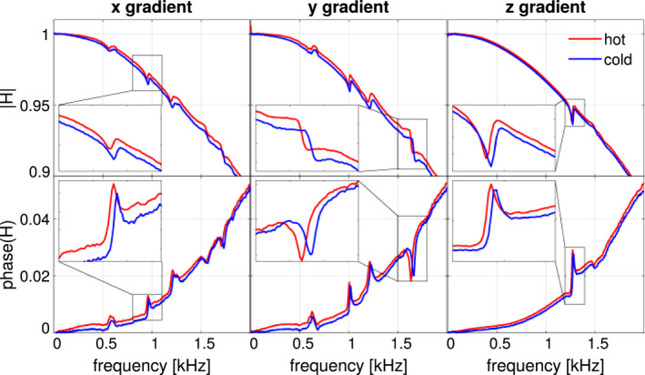
Examples of transfer functions observed in a hot state and the cold state. The chief effects of heating are a general increase and phase shift of the field response and downshift of mechanical resonances

3.3. Model self‐consistency and conditioning

Figure 4 shows the conditioning, self‐consistency, and prediction error of the thermal model as a function of temperature radius. With training as used in this study, the model is seen to be ill‐conditioned for radii smaller than $6^{\circ }$C. In this case, few of the temperature states visited during training lie within the temperature radius so that the matrix $\mathrm{\Delta }\widehat{\mathbf{T}}$ contains critically few columns, underdetermining the model. The conditioning settles beyond ${10}^{\circ }$C, indicating robust over‐determination. Even in the over‐determined regime, the condition number per se is still large. This is to be expected because temperature is naturally correlated between sensor positions, resulting in large first singular values of the training matrix. Under‐determination at low temperature radii is also reflected by exceeding self‐consistency (low ${\text{RMSE}}_{\text{SC}}$) and large prediction error. ${\text{RMSE}}_{\text{SC}}$ settles at 1.5–2.0 per mil for all gradient axes and the prediction errors settle at only somewhat larger values. Stable self‐consistency and prediction even at the largest radii indicate validity of the global linear model.

FIGURE 4.

Model conditioning, self‐consistency (${\text{RMSE}}_{\text{SC}}$) and ${\text{RMSE}}_{\mathit{total}}$ of prediction as functions of the temperature radius of the model. At small radius, ill‐conditioning and high self‐consistency indicate over‐fitting. Stable criteria beyond temperature radius of ${10}^{\circ }$C reflect robust modeling at prediction errors of 0.2–0.3 per mil. Stable criteria also at the largest temperature radii indicate validity of the global linear model

3.4. Global model

Figure 5 shows the performance of the global model in terms of prediction error as a function of frequency (${\text{RMSE}}_{\omega }$), compared with the deviation from the transfer function in the cold state. The model accuracy reaches almost the noise level with only small residual error predicting the behavior of mechanical resonances.

FIGURE 5.

Performance of the globally linear model in terms of prediction ${\text{RMSE}}_{\omega }$. Prediction accuracy reaches almost noise level. Subtle residual error remains only at the sites of mechanical resonances

The prediction performance of the global model is virtually independent of temperature as shown by the same criteria as functions of time in Figure 6. Error incurred by a reference taken in the cold state closely relates to the underlying temperature dynamics shown at the bottom of the figure. It converges back toward zero as the system returns to the cold state. The cool‐down and thus the convergence are slow, however, with multiple time constants up to the order of 10 min.

The figure also illustrates that heating changes the behavior not only of the gradient coil used for heating but of all coils, as may be expected due to thermal and mechanical coupling in the same structure. Nonetheless, heating by AC operation with the EPI sequences does affect the actually driven coil the most, unlike with DC heating. Notably, both DC and EPI heating via the actively cooled z coil alter the transfer functions substantially although the observed temperature changes remain moderate.

3.5. Local models

Figure 7 illustrates the transition from the globally linear model to locally linear models with temperature radii ranging from ${16}^{\circ }$C down to $5^{\circ }$C. As the plots show, the prediction performances of global and local modeling are broadly comparable. The local approach is somewhat superior at modeling thermal change of the mechanical resonances, suggesting that their largest shifts may breach the limits of global linear expansion. At $5^{\circ }$C radius, the local model starts to fail due to underdetermination as observed in Figure 4. In this data, the best radius is at about $7^{\circ }$C. However, in view of the moderate benefits of local modeling, only global modeling was used in the remainder of this study.

FIGURE 7.

Comparison of global and local modeling in terms of prediction ${\text{RMSE}}_{\omega }$. The two approaches perform broadly similarly. However, local modeling at the best temperature radius of $7^{\circ }$C is somewhat better at capturing changes in mechanical resonance effects

3.6. Choice of temperature sensors

Figure 8 reports the dependence of model performance on the underlying choice of temperature sensors. Use of all 19 sensors deployed in this study achieves the best predictions. However, notably, even a single well‐placed sensor such as the most predictive in‐bore sensor (#7) or one of the outflow sensors on the cooling circuit yield useful predictions, reducing error to the range of 20%–30% relative to the cold reference. Use of more sensors brings down the error significantly further and is helpful particularly for modeling mechanical resonances. Room temperature monitoring (not shown separately) added only negligible predictive value.

FIGURE 8.

Dependence of prediction error (${\text{RMSE}}_{\omega }$) on the placement and selection of temperature sensors, using the global model. The best results are achieved with all 19 sensors. However, even single‐sensor monitoring in‐bore or of outflowing cooling water reduces prediction error significantly relative to the cold reference (Figure 5)

3.7. Prediction of untrained scenarios

Figure 9 illustrates the necessity of training with different heating scenarios. The model performance deteriorates when training the model with only five of the six training sequences and using it to predict transfer functions observed after heating with the skipped sequence (Figure 9, top). However, upon use of all training sequences, that is, with both AC and DC heating via each of the gradient chains, thermal change was predicted rather well for the validation sequences with AC heating at lower or higher frequency than during training (Figure 9, bottom).

FIGURE 9.

Top: Prediction error (${\text{RMSE}}_{\omega }$) of x gradient transfer functions with incomplete training: One of the training sequences was excluded from model fitting and transfer functions after heating with the excluded sequence were predicted. For z gradient heating, the prediction still worked relatively well, but it failed for the others. Bottom: When relying on all training sequences, the heating effects of the validation sequences with untrained EPI readout frequencies were well predicted

3.8. Simulated imaging

Figure 10 shows the results of the imaging simulations along with the underlying trajectories. In the EPI trajectories, the strongest heating effect is oscillatory deviation in the readout direction, which is caused by change in both the transfer amplitude and the delay at the readout frequency. On‐resonance, large change in delay due to shifting of the resonance caused greater net trajectory differences, up to 0.2 times the sampling interval, although the maximum excursion of the trajectory deviates less from nominal than off‐resonance. Reconstructions based on cold‐state trajectories exhibit blurring and ghosting. The ghosting is stronger in the on‐resonance case, especially in the hot state, matching the change in delay. These artifacts are largely removed by reconstruction with model‐based trajectories, consistent with greatly reduced trajectory error (plotted in red). In the spiral case, the trajectory deviations are in the same order of magnitude while their effects at the image level are smaller. Artifacts are visible nonetheless, most clearly in the center of the brain, and again largely removed by reconstruction based on the thermal model.

FIGURE 10.

Simulated imaging in a warm state (${32}^{\circ }$C, left) and a hot state (${65}^{\circ }$C, middle), with three single‐shot readouts (from the top): EPI off any mechanical resonance, EPI on a resonance just below 1 kHz, and spiral. The shown images were obtained by reconstruction based on cold‐state transfer functions (“cold H”) and based on the thermal model (“model H”). Right: Effective trajectories in the cold state (blue), in the hot state (black), and according to the model (red), and their differences hot‐cold (“error cold,” blue) and hot‐model (“error model,” red). Bottom: spectra of the readout waveforms (x gradient), superimposed with error in the transfer function obtained with the model (black) vs the cold reference (grey)

4. DISCUSSION

According to the results of this study, performed with a typical clinical MRI system, gradient response undergoes relevant changes upon heating, which can well be estimated by thermal extension of the LTI model, treating heating as a linear perturbation.

Of the two main heating effects, the broadband increase of the transfer functions is approximately proportional to frequency in the low kHz range and goes along with an equally broadband phase shift. These characteristics suggest that the effect relates to eddy currents in the gradient coil conductors. Flowing in small local loops in copper at room temperature, such eddy currents are short‐lived, ⁴⁴ matching the broadband nature of the effect. With increasing resistivity as the copper heats up, the lifetimes of these eddy currents decrease further, reducing their shielding effect as seen in the data.

The other prominent heating effect observed here is a distinct downshift of mechanical resonances. The frequencies of the vibrational modes of the gradient tube depend, among others, on material properties. According to Refs. [45, 46], the eigenmode frequencies of hollow cylinders are proportional to the square root of Young’s modulus, which decreases with increasing temperature. ⁴⁷ , ⁴⁸ On this basis, the observed downshift likely reflects thermal softening of the gradient tube. Similarly, thermal increase in the loss module may cause stronger damping of vibration and thus broadening of the resonance peaks. However, this potential effect, if present, was too subtle to be observed in the present data.

It has been found that thermal change in transfer functions lends itself to linear expansion in terms of temperature, provided suitable temperature observables and adequate coverage of the temperature space by training scenarios. Notably, good prediction performance was achieved with global linear modeling, which is particularly convenient due to its simplicity and small demands in terms of training, storage, and computation. Good success of linear modeling indicates that thermal change is suitably small in the scale of the physics that relate temperature and field response. In general, these physics are not linear. For instance, the field effects of thermal shifts of mechanical resonances are linearizable only across a fraction of the peak width. This limit appears to have been nearly reached in this work, achieving somewhat better prediction of resonance shifts with local models. Local modeling is a viable option that overcomes the limits of global linearization. In turn, however, it requires more training data for suitable overdetermination within each local model range. Beyond linear models, one attractive future option is non‐linear parameterization of transfer functions incorporating knowledge of the physics involved. ⁴⁹

Irrespective of the chosen thermal model, sensing and training should target all temperature degrees of freedom that relate to changes in gradient response. In this work, infrared recordings were used to optimize temperature coverage by a large number of sensors. The implied coverage of field response variation was then assessed by predictions based on subsets of sensors. Notably, rather good modeling was achieved with few well‐placed sensors already. Nonetheless, the best results were obtained with the full set and model errors still remained, indicating that relevant thermal degrees of freedom were missed by the two‐step selection. To directly relate sets of sensor positions to their ability to encode change in field response, infrared imaging and measurement of transfer functions could be performed simultaneously. Temperature sensing on the cooling circuit has been found to be insufficient by itself but to improve results as a complement to sensing along the gradient tube.

Regarding training, it has been found to be critical to include both DC and AC heating, which generate different heating patterns due to different eddy current behavior. AC training at an intermediate frequency achieved rather good modeling of gradient response after heating with other frequencies, albeit not quite at the level observed with the same frequency. Similarly, good models resulted with few temperature sensors already, with diminishing returns of using the full set. Together, these findings indicate that much of the relevant thermal variation is limited to few degrees of freedom that can be probed and sampled with relatively few training scenarios and sensors.

Nonetheless, the training strategy calls for expansion and optimization beyond the initial set of training sequences used in this work. More extensive training will be time‐consuming but benefits greatly from real‐time recording of transfer functions as described in this work so that every heating scenario needs to be performed only once.

One immediate option for expansion is to probe more input frequencies, which will increase the spatial diversity of temperature patterns by varying the eddy current contribution to heating. Another scenario that will likely involve additional degrees of freedom is simultaneous heating by multiple gradient coils. With DC inputs, the generation of heat by each coil will still be independent of the others because each causes dissipation only within its own conductor. For linear heat transport, the resulting temperature patterns should then be linear superpositions of those obtained with one coil at a time and thus covered by per‐coil training. The situation is different, however, with AC inputs. For bulk current flowing along the coils, from terminal to terminal, the argument above still holds because the related dissipation is still limited to within each conductor. This is not true, however, of local eddy currents, which the switching of bulk current in any one of the coils induces not only in that same coil but also in the others. Upon simultaneous switching of multiple gradient coils, these eddy currents superimpose linearly. However, heat produced is proportional to the square of their sum and thus different from the sum of the heat each gradient chain alone would have generated. The number of relevant spatial degrees of freedom thus added remains to be investigated and considered in more advanced training strategies. Simultaneous intense AC operation is a scenario of practical importance because it occurs, for example, upon angulation of EPI readouts and with spiral scanning.

Training and use of models in this study have been limited to temperature distributions that occur during gradient cool‐down. However, the strategy explored here will equally apply with complementary training during heat‐up. The latter will entail interleaving of heating and response measurement intervals or, potentially, gradient waveforms that cover both functionalities.

In the present work, gradient characterization was performed with a field camera, permitting rapid measurement of transfer functions in under one second and at high frequency resolution of 5 Hz. Temporally resolved measurement is instrumental in capturing thermal system states, which are intrinsically transient. High frequency resolution has been found to be necessary to detect subtle changes in mechanical resonances. Alternatively, transfer functions can be measured with phantom‐based methods, ²⁸ , ³⁰ which should equally lend themselves to thermal modeling as described in Ref. [39] and in the present work, albeit at lower temporal resolution and ability to capture transient thermal states. Response measurement with a phantom has recently been deployed for studying temperature dependence. ⁵⁰ , ⁵¹ In this contribution, response data were averaged over 8 min at a time in approximate steady states, yielding transfer functions with frequency resolution of 100 Hz. Based on temperature readings from the MRI system used, transfer functions were shown to exhibit approximately linear temperature dependency at selected frequencies.

Thermal modeling of gradient response yields actual gradient dynamics during MR scans with greater accuracy than is available from calibration measurements in the cold state. It thus holds promise to improve image quality, particularly for long, gradient‐intensive scans with long 2D or even 3D readouts. A prominent example is BOLD fMRI with EPI readouts, which has been reported to suffer from thermal gradient drift, ⁵² , ⁵³ an observation supported by the imaging simulations reported here. Given temperature‐corrected transfer functions throughout an exam, actual k‐space trajectories can be computed from the nominal inputs and used for image reconstruction. On the same basis, pre‐emphasis could be temperature‐adjusted while scans are running. This approach should apply equally to the thermal characterization and pre‐emphasis of high‐order shim sets ³¹ , ⁴³ , ⁵⁴ as well as matrix‐ and other multiple‐coil arrangements. ⁵⁵ , ⁵⁶ , ⁵⁷ Unshielded or coupled setups may require the inclusion of cross‐term characterization ⁴³ , ⁵⁶ and modeling.

The actual field evolution during any MRI procedure can also be obtained by concurrent recording with NMR probes. ⁵⁸ Relative to this option, the thermal model exhibits somewhat lower accuracy, observed here as residual error in predicted transfer functions and slight artifact in reconstructed images. Unlike direct field measurement, it also requires reproducible system behavior and re‐training upon changes in hardware configuration. On the upside, once trained, the thermal model relies on just temperature measurement, which is comparatively simple and inexpensive, and fully independent of MR procedures.

CONFLICT OF INTEREST

Bertram Wilm and Benjamin Dietrich are employees of Skope Magnetic Resonance Technologies AG at the time of submission of this work. Klaas Pruessmann holds a research agreement with and receives research support from Philips. He is a shareholder of Gyrotools LLC.

Nussbaum J, Dietrich BE, Wilm BJ, Pruessmann KP. Thermal variation in gradient response: measurement and modeling. Magn Reson Med. 2022;87:2224–2238. doi: 10.1002/mrm.29123

REFERENCES

- 1. Mansfield P, Chapman B. Active magnetic screening of gradient coils in NMR imaging. J Magn Reson. 1986;66:573‐576. [Google Scholar]
- 2. Carlson JW, Derby KA, Hawryszko KC, Weideman M. Design and evaluation of shielded gradient coils. Magn Reson Med. 1992;26:191‐206. [DOI] [PubMed] [Google Scholar]
- 3. Turner R. Gradient coil design: a review of methods. Magn Reson Imaging. 1993;11:903‐920. [DOI] [PubMed] [Google Scholar]
- 4. Crozier S, Forbes LK, Roffmann WU, Luescher K, Doddrell DM. Currents and fields in shielded RF resonators for NMR/MRI. Meas Sci Technol. 1996;7:1083‐1086. [Google Scholar]
- 5. Alecci M, Jezzard P. Characterization and reduction of gradient‐induced eddy currents in the RF shield of a TEM resonator. Magn Reson Med. 2002;48:404‐407. [DOI] [PubMed] [Google Scholar]
- 6. Burl M, Young IR. Eddy currents and their control. In: Harris RK, Wasylishen R, eds. Encyclopedia of magnetic resonance. Chichester: John Wiley; 2007. ISBN 9780470034590. 10.1002/9780470034590.emrstm0147 [DOI] [Google Scholar]
- 7. Jensen DJ, Brey WW, Delayre JL, Narayana PA. Reduction of pulsed gradient settling time in the superconducting magnet of a magnetic resonance instrument. Med Phys. 1987;14:859‐862. [DOI] [PubMed] [Google Scholar]
- 8. Morich MA, Lampman DA, Dannels WR, Goldie FTD. Exact temporal eddy current compensation in magnetic resonance imaging systems. IEEE Trans Med Imaging. 1988;7:247‐254. [DOI] [PubMed] [Google Scholar]
- 9. Van Vaals JJ, Bergman AH. Optimization of eddy‐current compensation. J Magn Reson. 1990;90:52‐70. [Google Scholar]
- 10. Jehenson P, Westphal M, Schuff N. Analytical method for the compensation of eddy‐current effects induced by pulsed magnetic field gradients in NMR systems. J Magn Reson. 1990;90:264‐278. [Google Scholar]
- 11. Boesch C, Gruetter R, Martin E. Temporal and spatial analysis of fields generated by eddy currents in superconducting magnets: optimization of corrections and quantitative characterization of magnet/gradient systems. Magn Reson Med. 1991;20:268‐284. [DOI] [PubMed] [Google Scholar]
- 12. Liu Q, Hughes DG, Allen PS. Quantitative characterization of the eddy current fields in a 40‐cm bore superconducting magnet. Magn Reson Med. 1994;31:73‐76. [DOI] [PubMed] [Google Scholar]
- 13. Wysong RE, Madio DP, Lowe IJ. A novel eddy current compensation scheme for pulsed gradient systems. Magn Reson Med. 1994;31:572‐575. [DOI] [PubMed] [Google Scholar]
- 14. Kessels PHL. Understanding mechanical vibrations in MRI scanners. DCT rapporten. Vol. 1996. Eindhoven: Technische Universiteit Eindhoven; 1996:150. [Google Scholar]
- 15. Hedeen RA, Edelstein WA. Characterization and prediction of gradient acoustic noise in MR imagers. Magn Reson Med. 1997;37:7‐10. [DOI] [PubMed] [Google Scholar]
- 16. Mansfield P, Glover PM, Beaumont J. Sound generation in gradient coil structures for MRI. Magn Reson Med. 1998;39:539‐550. [DOI] [PubMed] [Google Scholar]
- 17. Doty FD. MRI gradient coil optimization. In: Blümler P, Blümich B, Botto R, Fukushima E, eds. Spatially Resolved Magnetic Resonance: Methods, Materials, Medicine, Biology, Rheology, Geology, Ecology, Hardware. Weinheim: Wiley‐VCH Weinheim; 1998:647‐674. [Google Scholar]
- 18. Hennel F, Girard F, Loenneker T. “Silent” MRI with soft gradient pulses. Magn Reson Med. 1999;42:6‐10. [DOI] [PubMed] [Google Scholar]
- 19. Clayton DB, Elliott MA, Leigh JS, Lenkinski RE. 1H spectroscopy without solvent suppression: characterization of signal modulations at short echo times. J Magn Reson. 2001;153:203‐209. [DOI] [PubMed] [Google Scholar]
- 20. Tomasi DG, Ernst T. Echo planar imaging at 4 Tesla with minimum acoustic noise. J Magn Reson Imaging. 2003;18:128‐130. [DOI] [PubMed] [Google Scholar]
- 21. Li W, Mechefske CK, Gazdzinski C, Rutt BK. Acoustic noise analysis and prediction in a 4‐T MRI scanner. Concepts Magn Reson. 2004;21B:19‐25. [Google Scholar]
- 22. Foerster BU, Tomasi D, Caparelli EC. Magnetic field shift due to mechanical vibration in functional magnetic resonance imaging. Magn Reson Med. 2005;54:1261‐1267. [DOI] [PMC free article] [PubMed] [Google Scholar]
- 23. Edelstein WA, Hedeen RA, Mallozzi RP, El‐Hamamsy S‐A, Ackermann RA, Havens TJ. Making MRI quieter. Magn Reson Imaging. 2002;20:155‐163. [DOI] [PubMed] [Google Scholar]
- 24. Mechefske CK, Yao G, Li W, Gazdzinski C, Rutt BK. Modal analysis and acoustic noise characterization of a 4T MRI gradient coil insert. Concepts Magn Reson. 2004;22B:37‐49. [Google Scholar]
- 25. Wu Y, Chronik BA, Bowen C, Mechefske CK, Rutt BK. Gradient‐induced acoustic and magnetic field fluctuations in a 4T whole‐body MR imager. Magn Reson Med. 2000;44:532‐536. [DOI] [PubMed] [Google Scholar]
- 26. Winkler SA, Schmitt F, Landes H. Gradient and shim technologies for ultra high field MRI. NeuroImage. 2018;168:59‐70. Neuroimaging with ultra‐high field MRI: present and future. [DOI] [PMC free article] [PubMed] [Google Scholar]
- 27. Cheng J, Gagoski B, Bolar D, et al. Gradient linear system modeling using gradient characterization. In: Proceedings of the International Society for Magnetic Resonance in Medicine. Vol. 16. 2008:1155. [Google Scholar]
- 28. Addy NO, Wu HH, Nishimura DG. Simple method for MR gradient system characterization and k‐space trajectory estimation. Magn Reson Med. 2012;68:120‐129. [DOI] [PMC free article] [PubMed] [Google Scholar]
- 29. Vannesjo SJ, Haeberlin M, Kasper L, et al. Gradient system characterization by impulse response measurements with a dynamic field camera. Magn Reson Med. 2013;69:583‐593. [DOI] [PubMed] [Google Scholar]
- 30. Rahmer J, Mazurkewitz P, Börnert P, Nielsen T. Rapid acquisition of the 3D MRI gradient impulse response function using a simple phantom measurement. Magn Reson Med. 2019;82:2146‐2159. [DOI] [PubMed] [Google Scholar]
- 31. Vannesjo SJ, Duerst Y, Vionnet L, et al. Gradient and shim pre‐emphasis by inversion of a linear time‐invariant system model. Magn Reson Med. 2017;78:1607‐1622. [DOI] [PubMed] [Google Scholar]
- 32. Vannesjo SJ, Graedel NN, Kasper L, et al. Image reconstruction using a gradient impulse response model for trajectory prediction. Magn Reson Med. 2016;76:45‐58. [DOI] [PubMed] [Google Scholar]
- 33. Chu KC, Rutt BK. MR gradient coil heat dissipation. Magn Reson Med. 1995;34:125‐132. [DOI] [PubMed] [Google Scholar]
- 34. While PT, Forbes LK, Crozier S. Calculating temperature distributions for gradient coils. Concept Magn Reson B. 2010;37 B:146‐159. [Google Scholar]
- 35. While PT, Poole MS, Forbes LK, Crozier S. Minimum maximum temperature gradient coil design. Magn Reson Med. 2013;70:584‐594. [DOI] [PubMed] [Google Scholar]
- 36. Freschi F, Sanchez Lopez H, Smith E, Tang F, Repetto M, Crozier S. Mixed‐dimensional elements in transient thermal analysis of gradient coils. Numer Heat Tr A‐Appl. 2016;69:265‐282. [Google Scholar]
- 37. Sabaté JA, Wang RR, Tao F, Chi S. Magnetic resonance imaging power: high‐performance MVA gradient drivers. IEEE Trans Emerg Sel Topics Power Electron. 2016;4:280‐292. [Google Scholar]
- 38. Kasper L, Bollmann S, Vannesjo SJ, et al. Monitoring, analysis, and correction of magnetic field fluctuations in echo planar imaging time series. Magn Reson Med. 2015;74:396‐409. [DOI] [PubMed] [Google Scholar]
- 39. Dietrich BE, Reber J, Brunner D, Wilm BJ, Pruessmann KP. Analysis and prediction of gradient response functions under thermal load. In: Proceedings of the International Society for Magnetic Resonance in Medicine. Scientific Meeting and Exhibition. Vol. 24. Singapore: ISMRM; 2016:3551. [Google Scholar]
- 40. Dietrich BE, Nussbaum J, Wilm BJ, Reber J, Pruessmann KP. Thermal variation and temperature‐based prediction of gradient response. In: Proceedings of the International Society for Magnetic Resonance in Medicine. Scientific Meeting and Exhibition. Vol 25. Honolulu; 2017:0079. [Google Scholar]
- 41. Nussbaum J, Wilm BJ, Dietrich BE, Pruessmann KP. Improved thermal modelling and prediction of gradient response using sensor placement guided by infrared photography. In: Proceedings of the International Society for Magnetic Resonance in Medicine. Scientific Meeting and Exhibition. Vol. 26. Paris; 2018:4210. [Google Scholar]
- 42. Dietrich BE, Brunner DO, Wilm BJ, et al. A field camera for MR sequence monitoring and system analysis. Magn Reson Med. 2016;75:1831‐1840. [DOI] [PubMed] [Google Scholar]
- 43. Vannesjo SJ, Dietrich BE, Pavan M, et al. Field camera measurements of gradient and shim impulse responses using frequency sweeps. Magn Reson Med. 2014;72:570‐583. [DOI] [PubMed] [Google Scholar]
- 44. Tang F. Gradient coil design and intra‐coil eddy currents in MRI systems (PhD thesis). The University of Queensland; 2016. [Google Scholar]
- 45. Arnold RN, Warburton GB. Flexural vibrations of the walls of thin cylindrical shells having freely supported ends. Proc R Soc London, Ser A. 1949;197:238‐256. [Google Scholar]
- 46. Greenspon JE. Flexural vibrations of a thick‐walled circular cylinder according to the exact theory of elasticity. J Aerospace Sci. 1960;27:37‐40. [Google Scholar]
- 47. Rösler J, Harders H, Bäker M. Elastisches verhalten. In: Mechanisches Verhalten der Werkstoffe. Wiesbaden: Springer; 2012:31‐62. [Google Scholar]
- 48. Ätzgrübchen Gottstein G. In Materialwissenschaften und Werkstofftechnik: Physikalische Grundlagen. Berlin Heidelberg: Springer; 2014. ISBN 978‐3‐642‐36602‐4. [Google Scholar]
- 49. Wilm BJ, Dietrich BE, Reber J, Vannesjo SJ, Pruessmann KP. Gradient response harvesting for continuous system characterization during MR sequences. IEEE T Med Imaging. 2019;1. [DOI] [PubMed] [Google Scholar]
- 50. Stich M, Pfaff C, Wech T, et al. Temperature‐dependent gradient system transfer function (GSTF). Proceedings of the International Society for Magnetic Resonance in Medicine. Scientific Meeting and Exhibition, vol. 27, Montreal, Canada; 2019:0443. [Google Scholar]
- 51. Stich M, Pfaff C, Wech T. Temperature‐dependent gradient system response. Magn Reson Med. 2020;83:1519‐1527. [DOI] [PubMed] [Google Scholar]
- 52. Giannelli M, Diciotti S, Tessa C, Mascalchi M. Effect of echo spacing and readout bandwidth on basic performances of EPI‐fMRI acquisition sequences implemented on two 1.5 T MR scanner systems. Med Phys. 2010;37:303‐310. [DOI] [PubMed] [Google Scholar]
- 53. Bollmann S, Kasper L, Vannesjo SJ, et al. Analysis and correction of field fluctuations in fMRI data using field monitoring. NeuroImage. 2017;154:92‐105. Cleaning up the fMRI time series: Mitigating noise with advanced acquisition and correction strategies. [DOI] [PubMed] [Google Scholar]
- 54. Jia F, Elshatlawy H, Aghaeifar A, et al. Design of a shim coil array matched to the human brain anatomy. Magn Reson Med. 2020;83:1442‐1457. [DOI] [PubMed] [Google Scholar]
- 55. Littin S, Jia F, Layton KJ, et al. Development and implementation of an 84‐channel matrix gradient coil. Magn Reson Med. 2018;79:1181‐1191. [DOI] [PubMed] [Google Scholar]
- 56. Ertan K, Taraghinia S, Atalar E. Driving mutually coupled gradient array coils in magnetic resonance imaging. Magn Reson Med. 2019;82:1187‐1198. [DOI] [PubMed] [Google Scholar]
- 57. Juchem C, Theilenberg S, Kumaragamage C, et al. Dynamic multicoil technique (DYNAMITE) MRI on human brain. Magn Reson Med. 2020;84:2953‐2963. [DOI] [PMC free article] [PubMed] [Google Scholar]
- 58. Wilm BJ, Barmet C, Pavan M, Pruessmann KP. Higher order reconstruction for MRI in the presence of spatiotemporal field perturbations. Magn Reson Med. 2011;65:1690‐1701. [DOI] [PubMed] [Google Scholar]