

Abstract
Autonomous and cabled platforms are revolutionizing our understanding of ocean systems by providing 4D monitoring of the water column, thus going beyond the reach of ship‐based surveys and increasing the depth of remotely sensed observations. However, very few commercially available sensors for such platforms are capable of monitoring large particulate matter (100–2000 μm) and plankton despite their important roles in the biological carbon pump and as trophic links from phytoplankton to fish. Here, we provide details of a new, commercially available scientific camera‐based particle counter, specifically designed to be deployed on autonomous and cabled platforms: the Underwater Vision Profiler 6 (UVP6). Indeed, the UVP6 camera‐and‐lighting and processing system, while small in size and requiring low power, provides data of quality comparable to that of previous much larger UVPs deployed from ships. We detail the UVP6 camera settings, its performance when acquiring data on aquatic particles and plankton, their quality control, analysis of its recordings, and streaming from in situ acquisition to users. In addition, we explain how the UVP6 has already been integrated into platforms such as BGC‐Argo floats, gliders and long‐term mooring systems (autonomous platforms). Finally, we use results from actual deployments to illustrate how UVP6 data can contribute to addressing longstanding questions in marine science, and also suggest new avenues that can be explored using UVP6‐equipped autonomous platforms.
Marine particles (mostly aggregates of organic and inorganic detritus and bacteria) and plankton are ubiquitous in the ocean and play important roles in biogeochemical cycles and trophic webs (Stemmann and Boss 2012; Turner 2015). In particular, several ecological services depend on biological processes largely mediated by marine particles and plankton (Ducklow et al. 2001; Travers et al. 2007; Rose et al. 2010). As a consequence, both particles and plankton have been recognized as biological Essential Oceanographic Variables (EOVs) for the Global Ocean Observing System (Miloslavich et al. 2018; Muller‐Karger et al. 2018). Observations of particles and phytoplankton rely, on the one hand, on particle‐collecting devices such as sediment traps that have been used for decades to assess the quantity and quality of settling marine snow in the ocean, but these can only resolve coarse spatial and temporal variations. On the other hand, in situ cameras deployed from ships have been used since the early 1990s to detect, measure, and identify marine particles and plankton in the size range of 100–2000 μm at high spatiotemporal resolution (Honjo et al. 1984; Lampitt et al. 1993; Ratmeyer and Wefer 1996). The imaging devices hold the promise of operationality and global consistency (Stemmann et al. 2012b; Lombard et al. 2019). An extensive review published by Lombard et al. (2019) has accordingly presented the different camera‐based systems available on the shelf, in which Underwater Vision Profiler (UVP) sensors were described along with other instruments, and their respective key characteristics were compared.
The UVP is unique in that it is the only intercalibrated camera‐based sensor that targets marine particles > 100 μm (in this paper, large particulate matter [LPM] corresponds to the 100–2000 μm range). The 5th model (UVP5), resulting from three decades of developments since the 1980s (Gorsky et al. 2000; Picheral et al. 2010), was small enough to be mounted inside most Conductivity, Temperature, Depth (CTD) Sensors frames (Picheral et al. 2010), enabling great progress to be made in understanding the sinking of organic particles and carbon sequestration, following the UVP5's deployment during oceanographic cruises at ocean mesoscales (Gorsky et al. 2002; Guidi et al. 2007; Waite et al. 2016), regional scales (Ramondenc et al. 2016), and the global scale (Guidi et al. 2015). In this way, the UVP led to the description of different types of aggregates, which were found to be linked with surface primary production (Roullier et al. 2014; Trudnowska et al. 2021). While not specifically developed to observe plankton, which are sometimes too rare or too small to be efficiently observed by it, this UVP nonetheless gave rise to major discoveries through in situ observations of rare and fragile plankton such as rhizarians (Biard et al. 2016; Stemmann et al. 2008a,b), planktonic polychaetes (Christiansen et al. 2018), Trichodesmium colonies (Guidi et al. 2012; Sandel et al. 2015), Arctic copepod communities (Vilgrain et al. 2021), and plankton communities more generally (Stemmann et al. 2008c; Forest et al. 2012). Yet despite extensive use of the UVP5 in the last decade (about 1000 casts per year since 2008), its more widespread use is limited by the difficulty of acquiring data in rough sea conditions and ice‐covered high latitudes where ship operations are difficult.
In parallel, the last decades have seen the emergence of autonomous platforms which are now used to remotely record temperature, salinity (Roemmich et al. 2009), and many other EOVs (Claustre et al. 2020). These platforms include autonomous underwater vehicles (AUVs), profiling floats (simply called “floats” hereinafter) and underwater gliders (simply called “gliders” hereinafter). The idea of deploying imaging sensors on autonomous platforms to provide global monitoring of particles and plankton was proposed a decade ago (Stemmann et al. 2012a), but technological constraints have hindered their implementation. While Ohman et al. (2019) have described a camera‐based zooplankton sensor for gliders, it has yet to be scaled up for general use. Specifically, the technical challenges of designing a camera‐based sensor that can be mounted on autonomous platforms are: miniaturization, low energy requirement to optimize the lifetime of the platform, and direct broadcast of data from the platform to the online repository. We therefore addressed the challenge of developing a camera‐based sensor mountable on gliders and floats, and simple enough to be produced commercially at a relatively low cost, bearing in mind that floats and their sensors are lost at the end of their useful lives. The targeted size range of particles varied from a few tens of micrometers to a few centimeters, encompassing marine snow and meso‐ and macro‐zooplankton. This way, our new imaging sensor could provide data for key EOVs on autonomous platforms.
In this paper, we provide details of the new, miniaturized UVP6s designed to meet our identified criteria and existing in two versions: the UVP6‐LP (low power) and the UVP6‐HF (high frequency). On the one hand, the UVP6‐LP is an off‐the‐shelf quantitative scientific imaging sensor specifically designed to be deployed on modern marine autonomous or cabled platforms, the latter including seabed observatories and remotely operated vehicles (ROVs). Its sensor is especially suited for platforms with low power and/or that are relatively small‐sized. While the UVP6‐HF uses the same optical system as the UVP6‐LP, it on the other hand images at a faster rate and thus requires more power, and is designed to be deployed on CTD rosettes and cruising AUVs.
Here, we provide information on the integration of the UVP6‐LP into gliders, floats, and long‐term mooring lines. We assess the quality of the resulting data by intercomparing the results of different UVP6s, and comparing them with those obtained with the UVP5 reference. Finally, we provide three examples from field deployments of UVP6s to demonstrate the relevance of their results to ocean ecosystem studies.
Materials and procedures
Materials
The UVP5 and UVP6
In all UVP models including versions 5 and 6, the objects imaged by the camera are illuminated by a lateral collimated light beam created in front of the lens (Fig. 1). All objects within this thin coherent sheet of light are imaged on a black background, which allows the UVP to easily detect and size them using a fixed threshold of pixel light intensity on the 8‐bit gray scale (called “threshold” in this manuscript) for image segmentation (i.e., the process by which a digital image is partitioned into various subgroups of pixels called image objects). Furthermore, all imaged particles within a fixed volume are in focus and at the same distance from the camera, thus enabling reliable size measurements as well as accurate determinations of particle and plankton concentrations.
Fig. 1.
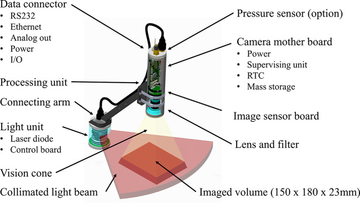
Diagram of the UVP6 camera and light unit.
Because the intensity of the light reflected by the particles can be high enough to activate pixels around the objects and because the light is also scattered and diffused in the path to the camera, a size compensation is applied when converting from pixels to metric units (Picheral et al. 2010). Results from the UVP thus depend on its optical tuning, fixed settings (black level, correction matrix, gain [amplification of the signal from the imaging sensor], shutter, transfer function, and threshold for segmentation) and additional calibration factors (called Aa and Exp, Eq. 1), which are used to convert pixel sizes (Sp) to calibrated metric size units (Smm) as follows:
| (1) |
The UVP6
The UVP6 is a miniaturized version of the UVP5 which relies on both a Supervising Unit and a Processing Unit with image‐acquisition capacity, detailed below. The major difference between the two models is the increased optimization of the UVP6 camera and light unit, thus decreasing the size of the longest dimension from 115 cm in the UPV5 to 50 cm in the UVP6‐LP, reducing the weight in air from 35 to 3.5 kg, and lowering the power consumption from 15 W to a maximum of 0.8 W.
The UVP6 consists of a main camera containing a mother board with a supervising processor, a mezzanine image processor unit, an image sensor board, a lens and a passband filter centered on 635 nm wavelength, and an optional pressure sensor. The light unit contains a controlling board, a laser diode and lenses, and is kept at a fixed distance from the camera by means of a connecting arm (Fig. 1).
The camera of the UVP6‐LP was designed with the purpose of achieving a fully dedicated hardware sensor. All design steps and choices were guided by the constraints of low power, small size, and reliability, to produce a sensor suitable for autonomous underwater platforms such as BGC‐Argo floats or moorings, which could operate during several years using only a fraction of the batteries powering the platform.
These choices led to a modular architecture, coordinated by a configurable Supervising Unit. This unit controls the Power Management subsystem which accepts power from 8 to 28 V, and is able to completely switch off the peripheral boards and devices and thus reduce quiescent consumption during idle periods. This way, the power consumption of the UVP6‐LP during long wait periods can be reduced to less than 10 mW on deployments where it cannot be electrically powered off, for example, on unsupervised moorings.
The Supervising Unit also deals with communications with the RS232 interface of the host platform as well as management of the optional pressure sensor and the antifouling devices. It can also drive a Digital‐to‐Analog‐Converter with a signal corresponding to the observed particle concentration. Finally, it coordinates the operation of the Processing Unit, which is the subsystem responsible for image acquisition, processing, and data storage.
The Processing Unit of the UVP6‐LP is based on a low‐power “FPGA‐SoC” device, which provides a suitable tradeoff between power consumption and processing power. Controlling both the image sensor and the light boards, this Processing Unit is able to precisely synchronize the image exposure with the laser flashes. It also takes care of data storage (400 GB microSD card media, 1 TB optional, which can host tens of millions of individual images), and has a 100 Mbps Ethernet interface used to download stored data without opening the camera housing.
As the Processing Unit is the most power‐consuming component of the UVP6, its operation is tightly regulated by the Supervising Unit to keep the mean power consumption as low as possible for a given acquisition frequency. For example, at the highest frequency allowed by the UVP6‐LP's Processing Unit of 1.3 frames per second (fps), its mean consumption is less than 1 W. This mean consumption is reduced to 100 mW when the UVP6‐LP is configured to process one image every 10 s (i.e., 0.1 fps).
The image sensor board of the UVP6 carries a 5 Mpixels CMOS monochrome image sensor (Sony IMX264) — a choice motivated by a tradeoff among several criteria that included resolution, pixel size, component size, light sensitivity, sensor noise, and power consumption. This choice also represents an upgrade in relation to the UVP5, currently existing in two versions: one with a 1.2 Mpixels CCD imager and the other with a 4 Mpixels CMOS imager.
The light board is synchronized with the image sensor's global electronic shutter which acquires all pixels at the same time. The light board also drives a laser diode emitting constant‐power red laser flashes (635 nm). Constant optical power is an extremely important feature that ensures the homogeneity of UVP6 data at different depths and water/sensor temperatures. The UVP6 light board thus has a temperature compensation circuit and can produce constant optical power flashes from 0°C to 35°C.
Finally, the UVP6 has a power back‐up system that makes it suitable for eventual functioning with a simple on/off controller. In this case, even if the input power were abruptly switched off, the camera has a power reserve to shut down gradually and thus avoid data losses and file system corruption.
The UVP6 firmware
Software development for the UVP6 followed the same objective as that for designing the hardware architecture, that is, achieving the best performance/power ratio without compromising data quality. A 2nd important feature was to provide a highly configurable and flexible UVP6, suitable for different types of deployments.
The Supervising Unit software implements a smart and dynamic resource‐managing algorithm, intended to optimize power consumption in real time according to the UVP6's workload. Furthermore, the high degree of configurability makes the UVP6 very versatile, that is, it can be used for cases ranging from the simplest power on/off to intricate autonomous acquisition schedules (AUTO and TIME main setup), including host (platform) controlled profiles that can be triggered on demand and in real time (SUPERVISED mode).
The Processing Unit software includes image‐ and data‐processing algorithms. It consists of three main processing steps: (1) light correction using a zone‐specific gain correction, (2) image segmentation, and (3) object/particle counting and characterization.
During the 1st step, in order to compensate for lighting differences between regions of the image, light‐correction (Fig. 2) processing is performed by the Processing Unit directly on the imager's pixel flow. A transfer function is also applied, which makes the sensor's sensitivity quasi‐logarithmic.
Fig. 2.
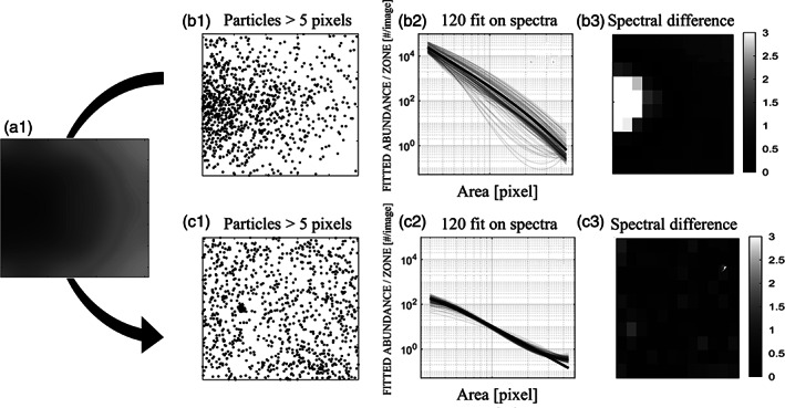
Examples of data from UVP6 000007LP showing the effect of zonal correction on the size spectra of particles: (a) image of the gain correction matrix to be applied to the raw image; (b) example of UVP6 data obtained without application of the correction matrix, presented here for illustrative purposes only; (c) real UVP6 data obtained after application of the correction matrix, with (1) position of selected particles, (2) size spectra in the 120 zones of the image, and (3) spectral differences in the 120 zones. The result of the application of the gain correction matrix is evaluated by the homogeneity among spectra in the 120 zones of the image (c2 and c3).
During the 2nd step, image segmentation is optimized for images that contain some sparse “white spots,” which correspond to objects/particles on a predominantly dark background. However, such optimization lends to strong performance penalties when it comes to very clear images (i.e., without white spots), which are most often caused by overexposure (typically near‐surface acquisition under bright sunlight). As overexposed images do not produce valid object counts, a fast preanalysis method is used to detect and eliminate these images, which prevents long processing times and associated energy expenditure. Segmentation of valid images produces a list of objects.
The 3rd processing step is to count and characterize the above objects, thus producing detailed data (counts for different sizes, mean pixel gray level, etc.) and a calibrated summary histogram (concentration per unit size, i.e., numbers per μm). Hence, according to the acquisition parameters, objects above a given size threshold (typically 620 μm, which corresponds to the usual size limit for the UVP5 and provides enough details for classification) can be extracted and stored as thumbnails (mass storage) for further analysis/classification (e.g., using the Ecotaxa software, Picheral et al. 2010).
In order to record the internal noise of the UVP6, which affects only very small objects (1 and 2 pixels), “black” images are acquired at preset intervals without activating the light, and the resulting data are saved along with the regular measurements.
In addition to differences in size, weight, and power consumption of the UVP6 compared to the UPV5, the Processing Unit of the UVP6‐LP has been optimized to boot in a few milliseconds to acquire and process a single image, whereas the UVP5 and the UVP6‐HF require 70 and 14 s, respectively, to boot their Processing Units. Other differences relate to the pixel size—145 and 88 μm for the two UVP5 versions offering different imagers but 73 μm for the UVP6‐LP and UVP6‐HF—and the imaged volumes, 1.1 and 0.7 L for the UVP5 and UVP6, respectively.
Procedures
Each UVP must be tuned in order to make its data comparable to those of other UVPs (i.e., sensor intercalibration), with the highest level of intercomparison achievable only through very careful tuning. We knew from the experience of intercalibrating the UVP5 that the optical tuning of the camera and the light unit are critical to obtain reliable and fully intercomparable sensors. It follows that the specific optical settings of each unit cannot be changed without losing the ability to compare its results with those of other units. We thus developed and tested a specific optical‐tuning procedure for the 1st two series of UVP6‐LP sensors, that is, seven prototypes built at the Laboratoire d'Oceanographie de Villefranche (LOV) in 2019, and 14 off‐the‐shelf sensors built by the Hydroptic company in 2020. All UVP5 and UVP6 settings, their tuning results and intercalibration results are recorded and saved in a dedicated and public database called UVPdb, which allows tracking of each sensor.
UVP6 light and camera tuning
The UVP6 camera tuning includes five steps: (1) optical centering of the sensor board using a specific target, (2) measurement of the imaging sensor's raw sensitivity, (3) tuning of the lens aperture to a defined sensitivity value equivalent to F4 when the best optical resolution is obtained, (4) tuning of the focusing of the imaging sensor, and (5) sensitivity tests after the UVP6 is finally assembled.
The UVP6 light tuning is performed on a calibration bench to compensate for the different lighting patterns created by heterogeneity among laser diodes. After the camera and light are assembled with a connecting arm, the rotation and centering of the camera relative to the light source are checked for each individual camera‐and‐light combination.
The UVP6 sensor is immersed in an aquarium filled with freshwater with the camera facing a white target placed at 45° in the light beam to measure the light beam's intensity and thickness. The resulting values are used to calculate the volume of the image captured by the camera, which corresponds to the intersection of the vision cone of the camera and the light beam (Fig. 1). The intensity of the light measured by the camera is used to adjust the flash and corresponding shutter duration of each UVP6 to compensate for differences among sensors and provide a fixed and common segmentation setting.
UVP6 optical compensation
The collimated light beam in front of the UVP6 camera is created from a single source (Fig. 1). As a consequence, despite the specific design of the lighting lens, the collimated light beam is still subject to significant radial divergence (Fig. 1). In addition, vignetting due to the camera lens is observed in the light intensity received by the UVP6 (i.e., lower intensity at the corners than in the center). Correction of this lighting heterogeneity cannot be achieved by theoretical modeling because of the complex properties of seawater and the very diverse types of objects (i.e., particles) imaged by the UVP6. For this reason, a method based on zonal correction of the image (Fig. 2) was developed to compensate for the UPV6's optical and lighting heterogeneity, with an empirical zone‐specific gain correction applied to the original images during the initial processing steps. This correction is designed to obtain identical size spectra (abundance of particles per size class) in each zone of the image for a given population of particles. To reach this goal, the image is divided into 120 zones (250 × 250 pixels) for which the local gain is selected after optimization (root mean square error [RMSE] minimization) and then interpolated over the whole image.
The efficiency of the gain zonal correction matrix is tested for each UVP6 during the intercalibration process by recording and analyzing the full raw images.
UVP6 intercalibration and comparison with UVP5
Intercalibration of reference UVP6s with reference UVP5
With the UVP6 being the successor of the UVP5, we wanted the two generations of UVPs to be highly comparable for the full range of particle sizes. We thus tuned the settings of the UVP6 on those of the UVP5, and created for this purpose three reference UVP6s to be used for all later intercalibrations.
Given that preliminary intercalibration experiments showed that three UVP6s built at LOV (i.e., sn000005lp, 000008lp, and 000010lp) provided very similar size spectra, we adjusted these three UVP6 to make them our references for future intercalibrations of all other UPV6 units (Fig. 3). The three UVP6s were attached to the same frame with a reference UVP5, which itself had been monitored over a number of years for its stability by comparisons with other UVP5. We lowered these four UVPs off Nice (Mediterranean Sea, France) at the speed of 0.5 m s−1 down to 250 or 500 m during six dives over a period of 3 weeks. The total volumes imaged by the three UVP6 ranged between 763 and 1232 L. After averaging the raw size spectra of all vertical profiles of each of the three UVP6s, we compared the resulting three sets of spectra with the averaged raw size spectra of the reference UVP5. Because the reference UVP5 had larger pixels than the UVP6s, we limited the size range of the intercalibration analysis to particles above 9 pixels for UVP5 and 24 pixels for UVP6, for which the abundance of objects began to be very similar, and we limited the upper sizes to classes in which a minimum of 30 objects were counted.
Fig. 3.
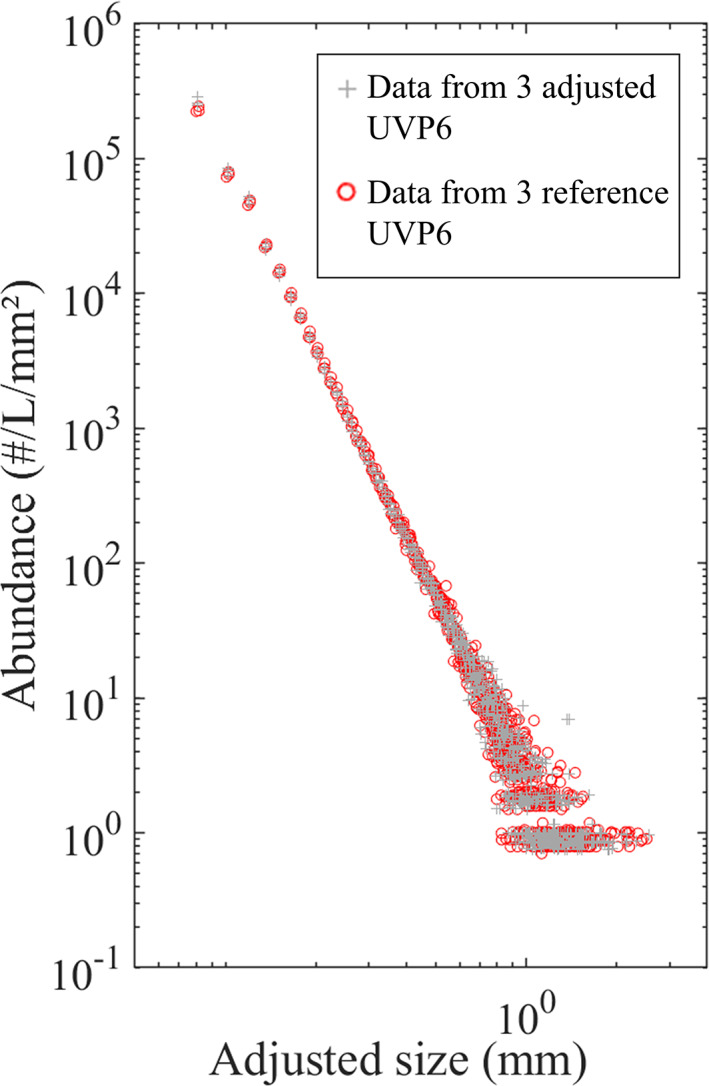
Example of results from an in situ intercalibration experiment. The particle spectra of three UVP6s (gray crosses, after adjustment during the in situ intercalibration experiments) are compared to those of the three UVP6 references (red circles).
We then determined the optimal threshold for each UVP6 as being the gray level for segmentation for which the RMSE between the raw particle size spectra of the UVP6 and the reference UVP5 was minimum. The final value of the optimum threshold was 20 on the 0–255 8‐bit gray scale for each of the three UVP6s.
We then computed the tuning parameters Aa and Exp (Eq. 1) of each UVP6 by minimizing the RMSE distance between the particle size spectra of UVP5 and UVP6. The small ranges of Aa (2271–2387) and Exp (1.130–1.143) show that the three UVP6 references produced almost identical results.
Intercalibration of the 1st two UVP6 series
Next, we used the same method to intercalibrate the 1st 18 UVP6s (4 others from LOV and 14 from Hydroptic), except that we averaged the size spectra of the three reference UVP6s instead of using the measurements from a single UVP5. In addition, given that all UVP6s had the same resolution, we extended the size range down to 3‐pixel objects. We did not count the 1‐ and 2‐pixel objects, which could have been impacted by sensor noise. As previously, we limited the upper size to those classes in which a minimum of 30 objects were counted.
Each UVP6 was lowered three times at sea, using a different shutter value each time (i.e., optimum, 15% lower, and 15% higher). For each shutter value, the optimum threshold for image segmentation was determined by minimizing the RMSE. The best shutter value was the one providing the closest optimum threshold above 20 (i.e., the optimum threshold of the three reference UVP6s) on the 8‐bit gray scale (0–255). This method ensured similar and limited noise for each UVP6. The Aa and Exp parameters (Eq. 1) were then adjusted for finer tuning.
The mean resulting threshold on the 8‐bit gray scale (0–255) for all the intercalibrated UVP6s was 20.6 (20–22), very close to the threshold for the three reference UVP6. This result indicated that the shutter correction and range were efficient at adjusting the different UVP6s, and that the UVP6s from LOV and Hydroptic did not differ.
We also compared the inter‐UVP6 distribution of RMSE between size spectra (particle abundance as a function of size expressed in Equivalent Spherical Diameter) for two different cases: (1) with the threshold tuning and using the mean Aa and Exp values of the reference UVP6s, and (2) with the threshold tuning and using and individually optimized Aa and Exp values for each UVP6. Optimizing the Aa and Exp parameters for each UVP6 led to a smaller RMSE, as expected. We noticed, however, that, in both cases, the RMSE was better than the RMSE of the three reference UVP6s. The optimization of Aa and Exp for each UVP6 was therefore not relevant, and we consequently favored a hardware calibration of the shutter and its corresponding threshold to obtain coherent results among UVP6s. Hence, the same averaged Aa and Exp parameters (i.e., 2300 and 1.1359, respectively) are used for all UVP6s. These parameters provide a lower detection size of 55 and 81 μm ESD for 1‐ and 2‐pixel targets, respectively.
Conclusion from the UVP6 intercalibration
The tuning of a UVP6 includes measurement of the light power and selection of the best shutter value and threshold of the 8‐bit gray scale close to 20 to fit the performance of the reference UVP6s. Even if the tuning procedure of the threshold values was limited to particle sizes up to 1 mm in the trials, these values could be extended by increasing the sampled water volume via deeper and/or repeated deployments. The matching of size spectra indicates that the detection of particles was identical for all UVP6s (Fig. 3).
The intercalibration statistics from 18 UVP6s indicate that the mean shutter was 318 ms at gain 6, the threshold was 20.6 (8‐bit gray 0–255 scale), and the RMSE for the reference size spectrum was 0.0028. The standard deviations for the shutter, the gain and the RMSE were 53 ms, 0.6 and 0.0019, respectively.
UVP6 integration setup for in situ deployment
The UVP6 has been designed to be easily integrated into different autonomous or cabled platforms, that is, in addition to its small size and low power consumption, it can start automatically after powering. It can also be fully piloted by the platform, to which it will generally be attached via the connecting arm between the camera and the light unit. Thanks to its RS232 and Ethernet interfaces, communication and downloading of data without opening the camera housing are possible and easy.
The UVP6‐LP has four main types of configuration setup: AUTO, TIME, SUPERVISED, and REMOTE CAMERA, the characteristics of which are summarized in Table 1. The four setups correspond to four types of deployments, each being possible on several platforms. The settings are based on a main hardware configuration table, 10 acquisition tables, and an optional timetable. The hardware configuration table primarily contains the sensor configuration (serial numbers of the camera and light, etc.), the main setup, the parameters resulting from tuning and intercalibration. The acquisition tables allow the selection of acquisition parameters including image rate, “black” intervals, and triggering method. Finally, the optional timetable allows selection of an acquisition table for each 30‐min deployment period when the UVP6 is utilized in TIME mode. Some of the settings have different options, which are summarized in Table 1.
Table 1.
Configurations and options of UVP6‐LP for deployment and use on different autonomous and cabled platforms.
| Main setup | Options | Deployment type | Host platforms |
|---|---|---|---|
|
AUTO UVP6 starts when powered ON, uses preset acquisition parameters |
AUTO UVP6 starts after a pre‐set delay, stops when OFF |
Any vector only capable of Power UVP ON and OFF |
Gliders* AUVs ROVs Landers Short‐term moorings |
|
TIME UVP6 starts acquisition according to a timetable loaded in the instrument |
TIME UVP6 starts after a pre‐set delay and check for programming every 30 min to start acquisition using up to 10 sets of parameters |
Long‐term deployments (week‐years) |
Landers Short‐, mid‐, and long‐term moorings |
|
SUPERVISED UVP6 waits for the hosting vector to start acquisition, sending a RS232 command to select the acquisition parameters |
CONTINUOUS UVP6 acquires images at its preset frequency |
Any vector capable of sending/receiving RS232 commands |
Gliders* Floats† AUVs ROVs Cabled observatories |
|
PILOTED UVP6 acquires images when triggered by the vector |
Any vector capable of sending/receiving RS232 “frequent” commands to trigger images |
Floats† Cabled observatories |
|
| REMOTE CAMERA | REMOTE CAMERA | Remote camera without image analysis through RS232 and ETHERNET (100 MB) | Experimental and connected remote station |
Presently Seaexplorer (Alseamar) and Seaglider (M1, Huntington Ingalls Industries; operated by Cyprus Subsea Consulting and Services C.S.C.S. Ltd) connected with the SIRMA™ smart cable.
Presently NKE CTS5‐USEA.
Data processing and management
General dataflow
The UVP6 takes advantage of an existing suite of software (UVPdb, UVPapp, EcoPart, and EcoTaxa) developed by LOV for image processing, data analysis and archiving (Fig. 4).
Fig. 4.
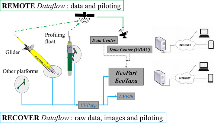
Dataflow pathways from UVP6 to users. REMOTE: Due to limited bandwidth, only selected and summarized data are transferred to the platform, and from the platform to land by satellite when the platform surfaces. RECOVER: The complete raw data and images are downloaded from the UVP6 mass storage via its Ethernet link using the UVPapp application. This 2nd dataflow applies to all platforms recovered after deployment.
UVPapp is an application for setting, piloting and programming the UVP6 in the different modes. It allows the setting of a frequency for the measurement of “black” images (i.e., images with no light), the downloading of data, the filling in of metadata, and the preparation of particle and images data for upload in EcoPart and Ecotaxa respectively. The UVPapp application is also designed to use the UVP6 as a remote camera for real‐time acquisition and visualization of images.
UVPdb is a web application that hosts all UVP5 and UVP6 settings and history from factory assembling to intercalibration. It can also be used for configuring the UVP6 via the UVPapp application and automatic calibrations and post‐processing in EcoPart.
EcoTaxa is a web application dedicated to the visual exploration and taxonomic annotation of images.
EcoPart is a web application linked to Ecotaxa which permits visualization and downloading of all types of UVP data. Currently, the EcoPart database holds 10,215 UVP5 and 6176 UVP6 profiles or time series of particle size spectra, and the Ecotaxa database hosts 48,000,000 images of particles and plankton (70–80% being non‐plankton particles) from most of the UVP profiles.
In cases when the UVP6 is recovered, the raw data and images can be downloaded via UVPapp, which allows the filling in of metadata and the selection of useful data prior to pre‐processing. When the UVP6 is mounted on and interfaced with a cabled or non‐recoverable platform, its data can either be displayed in real time (e.g., ship‐tethered ROVs) or stored and sent by satellite to Data Centers when the platform surfaces. The stored data can be either downloaded by users using EcoPart, which also allows for visualization and selection, or directly from the Data Center. For Argo floats, UVP6 data are decoded and made available in the AUX repository of the Global Data Assembly Center of the Argo project, which fosters the dissemination of these data.
CTS5 float dataflow
A specific integration procedure was designed for interfacing the UVP6‐LP with the CTS5 float from the NKE company in order to optimize all phases of data transmission from the UVP6 to the float. The transmitted data are the UVP6 metadata at the start of deployment, profiles of “black” measurements, and profiles of particle abundances and pixel gray levels. The UVPapp sets the UVP6 acquisition parameters to ensure optimal interaction with the float. The float firmware developed by NKE then selects the acquisition settings for up to five depth and parking zones and averages the data over variable depth ranges. A Graphical User Interface, also developed by NKE, allows estimation and optimization of the energy budget and the volume of transferred data to minimize satellite communication time and improve battery life. In addition, the float synchronizes the UVP6 time with its internal GPS time at the beginning of every profile, thereby facilitating the process of the raw data in the case of UVP6 recovery. Table 2 provides an example of recommended settings for float deployments, which represent a tradeoff between energy consumption, quantity of transferred data, and spatial resolution.
Table 2.
Recommended settings for deployments of UVP6 on floats for: (a) ascent profiles at 0.1 m s−1, (b) parking, and (c) resulting energy and dataflow budgets. The UVP6 is turned ON during ascending profiles from 2000 m to surface, and every 2 h for 400 s when at parking depth. The vertical speed is taken as 0.1 m s−1 during ascent. Particle data are averaged over different depth (z) ranges called slices.
| (a) Ascent profile settings | |||||||
|---|---|---|---|---|---|---|---|
| Zone | z range (decibar) | Time between images (s) | Pressure between images (dbar) | Width of LPM slice (dbar) | Imaged volume per slice (L) | Imaged volume per zone (L) | “Black” interval between images (#) |
| 1 | 0–2 | 10 | 1 | 2 | 1.26 | 1 | 10 |
| 2 | 2–100 | 3 | 0.3 | 5 | 17 | 326 | 10 |
| 3 | 100–500 | 3 | 0.3 | 10 | 33 | 1333 | 50 |
| 4 | 500–750 | 5 | 0.5 | 20 | 40 | 500 | 50 |
| 5 | 750–2000 | 5 | 0.5 | 20 | 40 | 2500 | 50 |
| (b) Parking settings | |||
|---|---|---|---|
| Parking total duration (min) | Acquisition interval (min) | Number of images per acquisition | Interval between images (s) |
| 13,000 | 120 | 20 | 20 |
| (c) Data and energy budget per dive | ||
|---|---|---|
| “Black” data (kB) | LPM data (kB) | Total power (kJ) |
| 6 | 24 | 5 |
Seaexplorer and Seaglider dataflow
The UVP6 has been interfaced with two types of gliders to date: Seaexplorer and Seaglider M1 (see footnote * in Table 1). These both require a UVP6 fitted with an optional pressure sensor. Both gliders synchronize the UVP6 clock with that of the glider at the start of each profile. Given that the gliders are recovered after missions, the importance of remotely transferred data is much lower than for floats, and only subsets of the data are thus sampled by the glider and transmitted for mission and data‐control purposes. Because glider missions and behaviors are much more diverse than those of floats, a very wide range of settings can be applied and no information is consequently provided in Table 3 (contrary to Table 2) on the data budget, the imaged volume per depth (z) range, and the energy budget.
Table 3.
Recommended settings for deployments on gliders for both ascent and descent profiles. Acquisition of data must be stopped at the surface and bottom of each profile to ease the processing of the recovered data.
| z range (decibar) | Time between images (s) | “Black” interval between images (#) |
|---|---|---|
| 0–100 | 3 | 10 |
| 100–500 | 3 | 50 |
| 500–750 | 5 | 50 |
| 750–2000 | 5 | 50 |
Assessment
UVP6 general controls
We used the 1st 21 UVP6‐LP units to check the model's functioning, its temperature compensation of light flashes, and UVP6 noise. Its clock drift was also checked, and proved to be less than 15 min/year, which is normal for this type of in situ instrument. The power consumption of the UVP6‐LP was found to be very low, that is, less than 1 W during the 750 ms required for image acquisition and processing, and less than 20 mW in between. Finally, the power back‐up system was extensively utilized and proved efficient at securing the end of data acquisition when the UVP6 is turned off.
UVP6 orientation on floats
For deployments on floats, we compared the vertical orientation of the sensors by mounting two UVP6s on the same float for three descent and three ascent profiles (down to 850, 650, and 470 decibars, respectively). The analysis of the results confirmed that down‐looking and up‐looking profiles provided the same information during both descent (0.03 m s−1) and typical float ascent (0.1 m/s), which was coherent with the fact that the float's very low speed prevents any wake effect. This result led to the decision to mount the UVP6 on floats looking downwards, as this orientation reduces the effect of direct sunlight on the images, and also prevents sinking particles from settling on the instrument's porthole.
Three case studies
We deployed UVP6 prototypes on different platforms. Here, we present examples of selected data from deployments on NKE CTS5 floats, a Seaexplorer glider in the Mediterranean Sea, and a mooring in the Arctic Ocean near Svalbard, Norway. All data were processed using UVPapp and imported in EcoPart and Ecotaxa after recovery, and also in quasi real time via satellite telemetry for the float and glider deployments. The data used for Figs. 5, 6, 7, 8, 9 were exported with EcoPart. The purpose here is not to analyze data in detail, but to provide examples of the possibilities provided by the UVP6 mounted on autonomous platforms. We also provide images of different particles and plankton recorded by the UVP6 to illustrate its imaging capability. The original data are available on the EcoPart and Ecotaxa websites.
Fig. 5.
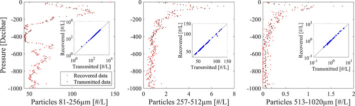
Particle abundance resulting from depth‐integrated data transmitted by satellite, and data recorded by the UVP6 sn000110LP and downloaded after retrieval of the float, for three selected size classes (from left to right, 81–256, 257–512, and 513–1020 μm) during a vertical profile down to 1000 m (1000 decibar) in the Mediterranean Sea off the coast of Nice (43.446°N, 7.187°E; 2020/07/21, 20:24 UTC). The figure shows the satellite‐transmitted data binned and displayed at variable depths of 5, 10 and 20 decibars according to LPM slices and the recovered data binned and displayed every 5 decibars.
Fig. 6.
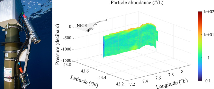
Left: UVP6‐LP mounted looking downwards on a NKE CTS5 BCG‐Argo float. Right: The abundance of particles from the 256 to 323 μm intermediate‐size class provided as an example during a 15‐profile float deployment in the Mediterranean Sea off Nice. The float drifted along the steep continental slope from 20 November 2019 to 25 November 2019.
Fig. 7.
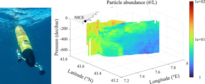
Left: UVP6‐LP mounted looking forward on a Seaexplorer glider, camera on the left and light on the right on the photo. Right: Abundance of particles from the 256 to 323 μm intermediate‐size class provided as an example during a 71‐dive deployment in the Mediterranean Sea off Nice, from 26 March 2019 to 29 March 2019. The glider transect was from the continental slope offshore.
Fig. 8.
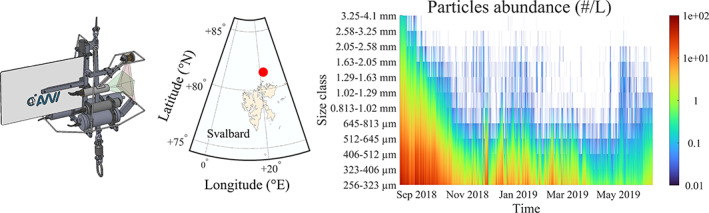
Left: UVP6‐LP mounted in its cage with other sensors. Center: Map showing the location of the mooring north of Svalbard during the INTAROS experiment (81.4772°N, 21.8867°W). Right: Abundance of particles in 11 selected size classes during the 10‐month deployment of the UVP6.
Fig. 9.
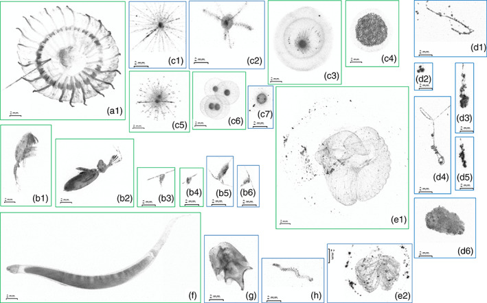
Examples of plankton and detritus images acquired by UVP6‐LP (blue frames) off the coast of Nice in March 2021, and UVP6‐HF (green frames) south of Tasmania during the Solace cruise in December 2020. The different organisms displayed are: (a1) a narcomedusa, (b1–b6) copepods, (c1–c7) rhizarian protozoa, (d1–d6) marine snow particles, (e1,e2) appendicularian houses, (f) a chaetognath, (g) a thecosome pteropod, and (h) a planktonic polychaete.
In the 1st case study, we mounted a UVP6 on a BGC‐Argo‐type profiling float (NKE CTS5), which was deployed on several occasions in the Mediterranean Sea off the coast of Nice, France, between April 2019 and July 2019 (Figs. 5, 6). These deployments were mostly intended to test the upward or downward orientation of the UVP6, the transfer of data between the UVP6 and the float, the satellite data transmission, and the coherence between the transmitted data and those downloaded after recovering the instrument. Maximum deployment duration was 30 d, with one vertical profile on each day. A maximum of 30 profiles was acquired during each deployment, corresponding to a virtual 10‐month deployment for a classic BGC‐Argo float profiling once every 10 d. Data transmitted by satellite, although averaged onboard the UVP6 over depth intervals, were not different from those downloaded after the float deployment (Fig. 5).
In the 2nd case study, we mounted the UVP6 on a Seaexplorer glider, and deployed it in the Mediterranean Sea off the coast of Nice. The glider was programmed to conduct two transects of 50 km each. The goal was to check whether the increased drag caused by the UVP6 impeded the efficiency of the glider, and if the latter could still perform its dives and efficiently orientate its path despite its modified hydrodynamics (Fig. 7). The piloting of the UVP6 at different depths and the transmission of UVP6 data were also tested. The glider successfully conducted the two transects, returning and waiting to be recovered at the set location despite a strong current. The UVP6 recorded 142 profiles during the 71 dives of the 1st transect (Fig. 7) and 396 profiles during the 198 dives of the 2nd transect (not illustrated).
In the 3rd case study, an early UVP6 prototype was deployed at 50 m depth on a 13‐month mooring (July 2018 to August 2019) in the Arctic Ocean north of Svalbard (INTAROS experiment, Fig. 8 ). This UVP6 continually and efficiently recorded numbers of particles and selected images of large targets every 40 s over the 1st 10 months of the deployment, until the aluminium arm broke due to corrosion (the parts of the UVP6 in contact with seawater are now solely made of titanium, plastic and glass).
In the three case studies, the UVP6 provided high‐resolution observations of particles. In the 1st study, the float drifted westward in the Ligurian current parallel to the coast, as expected. The concentration of particles was high at the surface and decreased progressively with depth (Figs. 5, 6), in a pattern typical for the region (Stemmann et al., 2002, 2008b). During the 2nd study, the glider observed a decreasing horizontal gradient from the coast offshore and a vertical gradient from the surface to 1000 m depth (Fig. 7), consistent with an earlier observation (Stemmann et al. 2008b). The UVP6 mounted on a float provided daily vertical variations of particles during 1 month, which have only been observed once in the past because of the ship time required (Stemmann et al. 2000). The UVP6 mounted on a glider provided details of the sharp boundary in the distribution of particles across the Ligurian Current, an area subject to complex horizontal and vertical hydrodynamics (Stemmann et al. 2008b). For the 3rd study in the Arctic Ocean, there were no previous data on particles acquired at such a frequency in the selected area. The results (Fig. 8) show a three‐step seasonal dynamic, with an initial decrease in particle concentration at the onset of winter, episodic particle bursts during winter which could correspond to sea‐ice dynamics, and the beginning of a particle rise in June possibly resulting from the settling of particles produced during the spring bloom.
Images of plankton and detritus
We provide in Fig. 9 examples of large plankton and particles (marine snow) obtained during several UVP6 deployments. The plankton images show that the camera resolution is high enough to distinguish morphological characteristics of millimetric objects, and thus identify their taxa. However, large plankton are generally rare in oceanic waters, that is, only a few per m3, and thus rarely appear on UVP6 images. As most of the imaged objects are smaller, only a minority of them can be identified from their morphological characteristics. The low abundance of large objects can be compensated by the repetition of sampling, thus providing enough data for quantitative ecological studies of plankton.
Discussion
During the last 30 years, data from UVPs have contributed to a better understanding of particle and plankton dynamics in the ocean. For example, results from UVP2 documented the export of particles in the northwestern Mediterranean Sea, and linked it to seasonal climatic forcing (Stemmann et al. 2002). Next, results from UVP2 and UVP4 highlighted the impact of mesoscale eddies on the spatial distribution of particle export in the Atlantic Ocean, the Indian Ocean and the Mediterranean Sea, and linked this phenomenon to the surface distribution of phytoplankton blooms (Stemmann et al. 2002; Guidi et al. 2007; Waite et al., 2016). Later, improvements to the imaging sensor and lighting system of the UVP4 enabled simultaneous estimation of vertical distributions of particles and zooplankton, and led to the 1st published comparison of mesopelagic macrozooplankton assemblages in a mesoscale context and across oceanic regions (Stemmann et al. 2008a,c). In addition, a global analysis of the complete database generated by the different UVPs showed that the size distribution of particles in the mesopelagic layer is closely related to the size distribution of phytoplankton in the euphotic zone (Guidi et al. 2009).
As of 2008, the UVP5 could be installed on CTD‐rosette frames and deployed together with other oceanographic sensors, that is, it no longer required stand‐alone deployments or dedicated ship time. Since then, the UVP5 has been deployed on average 1000 times per year, resulting in community progress in the study of key processes related to global and regional biological carbon pumps (Guidi et al. 2015; Ramondenc et al. 2016), macroplankton diversity in the upper kilometer of the ocean (Forest et al. 2012; Sandel et al. 2015; Biard et al. 2016; Christiansen et al. 2018), and fluxes of particles across coastal regions (Forest et al. 2013), in oxygen minimum zone areas (Roullier et al. 2014) and in the deep equatorial Pacific Ocean (Kiko et al. 2017). Other major improvements include software developments for both the streaming of data from UVPs to databases, and the automatic recognition of all types of objects (particles and plankton) on UVP images.
The “quantum leap” from UVP5 to UVP6 represents a major step forward in our ability to observe particles and plankton in the ocean. This is because the UVP6 can be mounted on floats, gliders and other autonomous or tethered platforms, thus allowing investigation of spatial and temporal particle and plankton dynamics at a high resolution that has been out of reach until now. The UVP6 has already been deployed down to 4500 m on Kiel6000 ROV, landers, bottom stations, sediment traps, and drifting arrays. Presently (2nd half of 2021), six UVP6 are profiling on CTS5 (BGC‐)Argo floats in the Indian, Atlantic, and Pacific Oceans, and three units are deployed on long‐term moorings in the Equatorial Atlantic and in the Wedel Sea.
Examples of what is now made possible by the UVP6 include deployments on moorings to capture the effects of rapid temporal events such as storms, periods of stratification, and destratification, or temporary intrusions of water masses on particles and plankton. Meanwhile, UV6s mounted on gliders can potentially survey the distributions of particles and plankton in and across physical features such as eddies, fronts, mesoscale filaments, or microlayers, which were difficult to capture with previous UVPs because of the required ship time. Otherwise, UVP6 mounted on BCG‐Argo floats together with other BGC sensors could provide long‐term information (up to 4 years if used in a classic BGC‐Argo float framework of about 350 cycles from 1000 m depth to the surface, or 200 cycles from 2000 m to the surface every 10 d), thus generating new understanding about seasonal and multi‐annual variations of biological activity in surface and intermediate waters and deep particle export. These examples represent only a fraction of what is achievable with the UVP6, as it may also be integrated into cabled benthic observatories, deployed in rivers, lakes, canals, industrial waters, used to monitor ballast water, as well as other applications not yet foreseen.
Comments and recommendations
The UVP6 is an optical sensor, and as such its optical surfaces need to remain clean and should be regularly checked to avoid biofouling and ensure data consistency when deployed in shallow water. Biofouling is limited on floats because their deep parking depth (≥ 1000 m) prevents colonization by biofilms. Our 1st observations show that the results from field deployments on the Svalbard mooring, floats and gliders (see above) were not impacted by any biofouling. In conditions where biofouling could occur, cleaning or protection devices for lenses or lighting could be interfaced using the input/output channel already present on the UVP6.
The present state of the UVP6 sensor leaves daytime vertical profiles open to impact by sunlight in the upper water column (e.g., down to 50 m in oceanic waters and at times of high sun elevation). This impact is nevertheless minimized by mounting the UVP facing down on floats as recommended above, which in addition prevents sinking particles from settling on the UVP's porthole. It is also recommended that the UVP6 be set to record “black” images at regular image‐acquisition intervals, that is, every 10 images above 100 m and every 50 deeper (default option in the acquisition tables; see above). The resulting information can be used to monitor the UVP6 noise for 1‐ and 2‐pixel particles, and possibly subtract it from the data afterward. The “black” measurements (i.e., acquired without activating the light) are also useful for detecting times when sunlight increases the noise levels on smaller particles (remnant overexposure), thus enabling definition of the useful depth for each profile below which the data are free from this bias.
When it is possible to recover the UVP6 after deployment (i.e., generally not the case when the UVP is mounted on a float), researchers can download the recorded images, which can generally not be transmitted by satellite. The downloaded data allow post‐calibration, and detailed identification of the objects on images. In addition, they give access to finer vertical resolution, which is voluntarily degraded to limit the amount of data transmitted by satellite and the duration of data transmission (the two dataflow pathways in Fig. 5).
The UVP6‐LP was developed for integration on autonomous vectors, hence our strategy of energy thriftiness. Results of the UVP6 are comparable to those of the UVP5 in terms of the abundance of small particles, but due to a lower acquisition rate and smaller imaged volume, larger objects including zooplankton could be rarer in UVP6‐LP data sets, as observed during our intercalibration experiments. The UVP6‐LP's slow acquisition rate resulting from energy limitation precludes its use on fast‐speed vectors such as AUVs and CTDs, for which we designed the UVP6‐HF. The latter sensor is now undergoing extensive tests on different cruises in the Pacific, Indian, Atlantic, and Arctic Oceans.
Acknowledgments
We acknowledge Prof. Gaby Gorsky who initiated the development of the UVP. We gratefully thank Ehsan Abdi, Emna Abidi, Florent Besson, Jean Yves Carval, Emilie Diamond, Laura Picheral, Louis Petiteau, Antoine Poteau and Christophe Schaeffer, for their assistance in the many technical experiments required for qualification of the UVP6. The development of the UVP6 was mainly funded by the European Union's Horizon 2020 research and innovation program under grant agreement no. 635359, project BRIDGES (Bringing together Research and Industry for the Development of Glider Environmental Services), and the GOPPI project of the “Programme Challenge Numérique” of the French Banque Publique d'Investissement and the Pôle Mer Méditerranée. LS was supported in the initial phase of the development by the CNRS/Sorbonne University Chair VISION. The integration of the UVP6 on the NKE CTS5 float was partly funded by the ERC REFINE (European Research Council, grant agreement 834177). We acknowledge funding by the H2020 project INTAROS (Integrated Arctic observation system; grant no. 727890) and the PACES (Polar Regions and Coasts in a Changing Earth System) Program of the Helmholtz Association.
Associate editor: Ivona Cetinic
Contributor Information
Marc Picheral, Email: marc.picheral@imev-mer.fr.
Lars Stemmann, Email: lars.stemmann@imev-mer.fr.
References
- Biard, T. , and others . 2016. In situ imaging reveals the biomass of giant protists in the global ocean. Nature 532: 504. doi: 10.1038/nature17652 [DOI] [PubMed] [Google Scholar]
- Christiansen, S. , and others . 2018. Particulate matter flux interception in oceanic mesoscale eddies by the polychaete Poeobius sp. Limnol. Oceanogr. 63: 2093–2109. doi: 10.1002/lno.10926 [DOI] [Google Scholar]
- Claustre, H. , Johnson K. S., and Takeshita Y.. 2020. Observing the global ocean with biogeochemical‐Argo. Ann. Rev. Mar. Sci. 12: 23–48. doi: 10.1146/annurev-marine-010419-010956 [DOI] [PubMed] [Google Scholar]
- Ducklow, H. W. , Steinberg D. K., and Buesseler K. O.. 2001. Upper ocean carbon export and the biological pump. Oceanogr. Wash. DC Oceanogr. Soc. 14: 50–58. doi: 10.5670/oceanog.2001.06 [DOI] [Google Scholar]
- Forest, A. , Stemmann L., Picheral M., Burdorf L., Robert D., Fortier L., and Babin M.. 2012. Size distribution of particles and zooplankton across the shelf‐basin system in southeast Beaufort Sea: Combined results from an Underwater Vision Profiler and vertical net tows. Biogeosciences 9: 1301–1320. doi: 10.5194/Bg-9-1301-2012 [DOI] [Google Scholar]
- Forest, A. , and others . 2013. Ecosystem function and particle flux dynamics across the Mackenzie Shelf (Beaufort Sea, Arctic Ocean): An integrative analysis of spatial variability and biophysical forcings. Biogeosciences 10: 2833–2866. doi: 10.5194/bg-10-2833-2013 [DOI] [Google Scholar]
- Gorsky, G. , Picheral M., and Stemmann L.. 2000. Use of the Underwater Video Profiler for the study of aggregate dynamics in the North Mediterranean. Estuar. Coast. Shelf Sci. 50: 121–128. doi: 10.1006/ecss.1999.0539 [DOI] [Google Scholar]
- Gorsky, G. , Prieur L., Taupier‐Letage I., Stemmann L., and Picheral M.. 2002. Large particulate matter in the Western Mediterranean: I. LPM distribution related to mesoscale hydrodynamics. Journal of Marine Systems 33: 289–311. doi: 10.1016/S0924-7963(02)00063-5 [DOI] [Google Scholar]
- Guidi, L. , Stemmann L., Legendre L., Picheral M., Prieur L., and Gorsky G.. 2007. Vertical distribution of aggregates (> 110 μm) and mesoscale activity in the northeastern Atlantic: Effects on the deep vertical export of surface carbon. Limnol. Oceanogr. 52: 7–18. doi: 10.4319/lo.2007.52.1.0007 [DOI] [Google Scholar]
- Guidi, L. , Stemmann L., Jackson G. A., Ibanez F., Claustre H., Legendre L., Picheral M., and Gorsky G.. 2009. Effects of phytoplankton community on production, size and export of large aggregates: A world‐ocean analysis. Limnol. Oceanogr. 54: 1951–1963. doi: 10.4319/lo.2009.54.6.1951 [DOI] [Google Scholar]
- Guidi, L. , Calil P. H., Duhamel S., Björkman K. M., Doney S. C., Jackson G. A., Li B., Church M. J., Tozzi S., Kolber Z. S., and Richards K. J.. 2012. Does eddy‐eddy interaction control surface phytoplankton distribution and carbon export in the North Pacific Subtropical Gyre? J. Geophys. Res. Biogeosci. 117: G02024. doi: 10.1029/2012JG001984 [DOI] [Google Scholar]
- Guidi, L. , Legendre L., Reygondeau G., Uitz J., Stemmann L., and Henson S. A.. 2015. A new look at ocean carbon remineralization for estimating deepwater sequestration. Global Biogeochem. Cycles 29: 1044–1059. doi: 10.1002/2014gb005063 [DOI] [Google Scholar]
- Honjo, S. , Doherty K. W., Agrawal Y. C., and Asper V. L.. 1984. Direct optical assessment of large amorphous aggregates (marine snow) in the Deep Ocean. Deep Sea Res. Part Oceanogr. Res. Pap. 31: 67–76. doi: 10.1016/0198-0149(84)90073-6 [DOI] [Google Scholar]
- Kiko, R. , and others . 2017. Biological and physical influences on marine snowfall at the equator. Nat. Geosci. 10: 852. doi: 10.1038/ngeo3042 [DOI] [Google Scholar]
- Lampitt, R. S. , Hillier W. R., and Challenor P. G.. 1993. Seasonal and diel variation in the open ocean concentration of marine snow aggregates. Nature 362: 737–739. doi: 10.1038/362737a0 [DOI] [Google Scholar]
- Lombard, F. , and others . 2019. Globally consistent quantitative observations of planktonic ecosystems. Front. Mar. Sci. 6: 196. doi: 10.3119/fmars.2019.00196 [DOI] [Google Scholar]
- Miloslavich, P. , and others . 2018. Essential ocean variables for global sustained observations of biodiversity and ecosystem changes. Glob. Change Biol. 24: 2416–2433. doi: 10.1111/gcb.14108 [DOI] [PubMed] [Google Scholar]
- Muller‐Karger, F. E. , and others . 2018. Advancing marine biological observations and data requirements of the complementary essential ocean variables (EOVs) and essential biodiversity variables (EBVs) frameworks. Front. Mar. Sci. 5: 211. [Google Scholar]
- Ohman, M. D. , Davis R. E., Sherman J. T., Grindley K. R., Whitmore B. M., Nickels C. F., and Ellen J. S.. 2019. Zooglider: An autonomous vehicle for optical and acoustic sensing of zooplankton. Limnol. Oceanogr. Methods 17: 69–86. doi: 10.1002/lom3.10301 [DOI] [Google Scholar]
- Picheral, M. , Guidi L., Stemmann L., Karl D. M., Iddaoud G., and Gorsky G.. 2010. The Underwater Vision Profiler 5: An advanced instrument for high spatial resolution studies of particle size spectra and zooplankton. Limnol. Oceanogr.Methods 8: 462–473. doi: 10.4319/lom.2010.8.462 [DOI] [Google Scholar]
- Ramondenc, S. , MadeleineGoutx F., Lombard C., Santinelli L., Stemmann G. G., and Guidi L.. 2016. An initial carbon export assessment in the Mediterranean Sea based on drifting sediment traps and the Underwater Vision Profiler data sets. Deep‐Sea Res. Part Oceanogr. Res. Pap. 117: 107–119. doi: 10.1016/j.dsr.2016.08.015 [DOI] [Google Scholar]
- Ratmeyer, V. , and Wefer G.. 1996. A high resolution camera system (ParCa) for imaging particles in the ocean: System design and results from profiles and a three‐month deployment. J. Mar. Res. 54: 589–603. doi: 10.1357/0022240963213565 [DOI] [Google Scholar]
- Roemmich, D. , Johnson G. C., Riser S., Davis R., Gilson J., Owens W. B., Garzoli S. L., Schmid C., and Ignaszewski M.. 2009. The Argo program observing the Global Ocean with profiling floats. Oceanography 22: 34–43. doi: 10.5670/oceanog.2009.36 [DOI] [Google Scholar]
- Rose, K. A. , and others . 2010. End‐to‐end models for the analysis of marine ecosystems: Challenges, issues, and next steps. Mar. Coast. Fish. 2: 115–130. doi: 10.1577/C09-059.1 [DOI] [Google Scholar]
- Roullier, F. , Berline L., Guidi L., De Madron X. D., Picheral M., Sciandra A., Pesant S., and Stemmann L.. 2014. Particle size distribution and estimated carbon flux across the Arabian Sea oxygen minimum zone. Biogeosciences 11: 4541–4557. doi: 10.5194/bg-11-4541-2014 [DOI] [Google Scholar]
- Sandel, V. , Kiko R., Brandt P., Dengler M., Stemmann L., Vandromme P., Sommer U., and Hauss H.. 2015. Nitrogen Fuelling of the Pelagic Food Web of the Tropical Atlantic. PLoS One 10: e0131258. doi: 10.1371/journal.pone.0131258 [DOI] [PMC free article] [PubMed] [Google Scholar]
- Stemmann, L. , Picheral M., and Gorsky G.. 2000. Diel variation in the vertical distribution of particulate matter (> 0.15 mm) in the NW Mediterranean Sea investigated with the Underwater Video Profiler. Deep‐Sea Res. Part I Oceanogr. Res. Pap. 47: 505–531. doi: 10.1016/S0967-0637(99)00100-4 [DOI] [Google Scholar]
- Stemmann, L. , Gorsky G., Marty J. C., Picheral M., and Miquel J. C.. 2002. Four‐year study of large‐particle vertical distribution (0–1000 m) in the NW Mediterranean in relation to hydrology, phytoplankton, and vertical flux. Deep‐Sea Res. Part II Top. Stud. Oceanogr. 49: 2143–2162. doi: 10.1016/S0967-0645(02)00032-2 [DOI] [Google Scholar]
- Stemmann, L. , Hosia A., Youngbluth M. J., Soiland H., Picheral M., and Gorsky G.. 2008a. Vertical distribution (0–1000 m) of macrozooplankton, estimated using the Underwater Video Profiler, in different hydrographic regimes along the northern portion of the Mid‐Atlantic Ridge. Deep‐Sea Res. Part II Top. Stud. Oceanogr. 55: 94–105. doi: 10.1016/j.dsr2.2007.09.019 [DOI] [Google Scholar]
- Stemmann, L. , Prieur L., Legendre L., Taupier‐Letage I., Picheral M., Guidi L., and Gorsky G.. 2008b. Effects of frontal processes on marine aggregate dynamics and fluxes: An interannual study in a permanent geostrophic front (NW Mediterranean). J. Mar. Syst. 70: 1–20. [Google Scholar]
- Stemmann, L. , and others . 2008. Global zoogeography of fragile macrozooplankton in the upper 100‐1000 m inferred from the underwater video profiler. Ices J. Mar. Sci. 65: 433–442. doi: 10.1093/icesjms/fsn010 [DOI] [Google Scholar]
- Stemmann, L. , and Boss E.. 2012. Plankton and particle size and packaging: From determining optical properties to driving the biological pump. Ann. Rev. Mar. Sci. 4: 263–290. doi: 10.1146/Annurev-Marine-120710-100853 [DOI] [PubMed] [Google Scholar]
- Stemmann, L. , Claustre H., and D'ortenzio F.. 2012a. Integrated observation system for pelagic ecosystems and biogeochemical cycles in the oceans. Sens. Ecol. Integr. Knowl. Ecosyst. 1: 261–278. [Google Scholar]
- Stemmann, L. , Picheral M., Guidi L., Lombard F., Prejger F., Claustre H., and Gorsky G.. 2012b. Assessing the spatial and temporal distributions of zooplankton and marine particles using the Underwater Vision Profiler. Sens. Ecol. 119: 119–137. [Google Scholar]
- Travers, M. , Shin Y.‐J., Jennings S., and Cury P.. 2007. Towards end‐to‐end models for investigating the effects of climate and fishing in marine ecosystems. Prog. Oceanogr. 75: 751–770. doi: 10.1016/j.pocean.2007.08.001 [DOI] [Google Scholar]
- Trudnowska, E. , and others . 2021. Marine snow morphology illuminates the evolution of phytoplankton blooms and determines their subsequent vertical export. Nat. Commun. 12: 2816. doi: 10.1038/s41467-021-22994-4 [DOI] [PMC free article] [PubMed] [Google Scholar]
- Turner, J. T. 2015. Zooplankton fecal pellets, marine snow, phytodetritus and the ocean's biological pump. Prog. Oceanogr. 130: 205–248. doi: 10.1016/j.pocean.2014.08.005 [DOI] [Google Scholar]
- Vilgrain, L. , Maps F., Picheral M., Babin M., Aubry C., Irisson J., and Ayata S.. 2021. Trait‐based approach using in situ copepod images reveals contrasting ecological patterns across an Arctic ice melt zone. Limnol. Oceanogr. 66(4): 1155–1167. doi: 10.1002/lno.11672 [DOI] [Google Scholar]
- Waite, A. M. , Stemmann L., Guidi L., Calil P. H. R., Hogg A. M. C., Feng M., Thompson P. A., Picheral M., and Gorsky G.. 2016. The wineglass effect shapes particle export to the deep ocean in mesoscale eddies. Geophys. Res. Lett. 43: 9791–9800. doi: 10.1002/2015gl066463 [DOI] [Google Scholar]