Tracking Strain‐Specific Morphogenesis and Angiogenesis of Murine Calvaria with Large‐Scale Optoacoustic and Ultrasound Microscopy

ABSTRACT

Skull bone development is a dynamic and well‐coordinated process playing a key role in maturation and maintenance of the bone marrow (BM), fracture healing, and progression of diseases such as osteoarthritis or osteoporosis. At present, dynamic transformation of the growing bone (osteogenesis) as well as its vascularization (angiogenesis) remain largely unexplored due to the lack of suitable in vivo imaging techniques capable of noninvasive visualization of the whole developing calvaria at capillary‐level resolution. We present a longitudinal study on skull bone development using ultrasound‐aided large‐scale optoacoustic microscopy (U‐LSOM). Skull bone morphogenesis and microvascular growth patterns were monitored in three common mouse strains (C57BL/6J, CD‐1, and Athymic Nude‐Foxn1nu) at the whole‐calvaria scale over a 3‐month period. Strain‐specific differences in skull development were revealed by quantitative analysis of bone and vessel parameters, indicating the coupling between angiogenesis and osteogenesis during skull bone growth in a minimally invasive and label‐free manner. The method further enabled identifying BM‐specific sinusoidal vessels, and superficial skull vessels penetrating into BM compartments. Our approach furnishes a new high‐throughput longitudinal in vivo imaging platform to study morphological and vascular skull alterations in health and disease, shedding light on the critical links between blood vessel formation, skull growth, and regeneration. © 2022 The Authors. Journal of Bone and Mineral Research published by Wiley Periodicals LLC on behalf of American Society for Bone and Mineral Research (ASBMR).

Introduction

Angiogenesis and vascular remodeling are key contributors to calvaria growth^{( 1} , ² , ^{3 )} and repair.^{( 4} , ^{5 )} The bone vascular network not only carries cells, oxygen, nutrients, and waste, but also plays an active role in the development and maintenance of bone marrow (BM) tissue serving as niches for hematopoietic stem cells and perivascular osteoprogenitors.^{( 2} , ⁶ , ^{7 )} Bone vascular morphology abnormalities further underlie major ailments such as osteoarthritis and osteoporosis. Thus, an accurate characterization of the bone vascular network is crucial to understanding disease mechanisms and monitoring therapeutic outcomes. In addition, osteogenesis, the process induced by osteoblasts, is essential for not only new bone growth but also regenerative fracture healing.^{( 4} , ^{5 )} Understanding its coupling with angiogenesis is indispensable for exploring mechanisms underlying skull development. Furthermore, through their connection to BM vascular networks, bone‐associated vessels contribute to the regulation of oxygenation, metabolic status, and, hence, hematopoietic function of the BM.

Despite its physiological importance, dynamics of vascular morphology during murine skull development remain poorly understood. Beyond limited ex vivo studies,^{( 8 )} imaging the large vascular network within highly heterogeneous and optically scattering skull bone remains challenging.^{( 7} , ⁹ , ^{10 )} Cerebral vessels in mice can be imaged with micro–magnetic resonance imaging (μMRI)^{( 11 )} and micro–computed tomography (μCT),^{( 12 )} but resolving skull microvasculature in vivo and longitudinally remains challenging with these modalities, especially for vessels <30 μm in diameter. Intravital optical techniques, such as confocal and two‐photon microscopy, are among the preferred techniques for interrogating the skull because of their high spatial resolution and large diversity of the available fluorescent markers.^{( 6} , ⁷ , ¹³ , ^{14 )} However, in vivo imaging with these techniques is conventionally limited to submillimeter areas, thus necessitating lengthy depth tiling and image stitching procedures to visualize larger skull areas.^{( 10 )} This time‐consuming process hinders high‐throughput studies on large‐scale (e.g., the whole calvaria) vascular networks further involving multiple mice and strains.

Optoacoustic (OA) imaging visualizes tissue chromophores by detecting tiny ultrasound (US) vibrations induced by absorption of short‐duration light pulses.^{( 15} , ^{16 )} In particular, in its optical‐resolution embodiment, focused illumination has been used to achieve capillary‐level resolution at whole‐brain scale.^{( 17} , ^{18 )} Detection of time‐resolved US signals then enables the volumetric visualization of optical tissue contrast (primarily stemming from hemoglobin) without the need of depth scanning to attain three‐dimensional (3D) information. When combined with pulse‐echo US imaging, complementary information on the skull bone morphology (e.g., skull shape and thickness) allows the label‐free segmentation of skull and brain vascular networks.^{( 19 )} OA microscopy has been shown to be capable of imaging healthy vasculature and tumor angiogenesis in murine ear and brain.^{( 20} , ^{21 )} In addition, hybrid implementations combining US biomicroscopy have revealed skull‐wide effects of radiation therapy.^{( 19 )}

Here, we report on the first longitudinal study of skull bone morphogenesis and vascular development patterns using US‐aided large‐scale OA microscopy (U‐LSOM). The study was performed in three common mouse strains, namely C57BL/6J, CD‐1, and Athymic Nude‐Foxn1nu (abbreviated as Nude), revealing the coupling between angiogenesis and osteogenesis, as well as differences in the skull bone development timeframe among strains over a 3‐month period. With effective penetration beyond 1 mm in vivo, the technique could be used to render the skull, BM, and cortical vasculature within a single scan with 7.5 μm lateral resolution, further enabling long‐term monitoring of skull bone morphogenesis owing to the additional pulse‐echo US imaging capability.

Materials and Methods

Ultrasound‐aided large‐scale optoacoustic microscopy (U‐LSOM)

The schematic of the U‐LSOM system used for imaging the skull bone is shown in Fig. 1A. A pulsed nanosecond‐duration laser (Onda; Bright Solutions, Prado, Italy) operated at 532 nm wavelength was used to generate 900 nJ per‐pulse energy (PPE). A small fraction of the laser light was guided into a photodetector to monitor and correct for PPE fluctuations. Focused laser light was delivered onto the mouse head through a single‐mode fiber and a gradient index (GRIN) lens with 7.5 mm focal distance (Grintech, Jena, Germany), which is mounted into a central hole of a single‐element spherically focused polyvinylidene fluoride (PVDF) transducer with 35 MHz central frequency and >100% effective bandwidth (Precision Acoustics, Dorchester, UK). The low numerical aperture (NA = 0.025) of the GRIN lens results in an effective depth range beyond 1 mm, thus enabling volumetric imaging of the curved skull and brain without necessitating depth scanning while achieving concentric illumination and acoustic detection for optimal detection sensitivity. The LSOM and pulse‐echo US modalities share the same scanning mechanism, transducer and receiver electronics, resulting in naturally co‐registered volumetric datasets.

All acquired image datasets were first bandpass‐filtered between 1 MHz and 100 MHz using a first‐order Butterworth filter. To compensate for laser PPE fluctuations, OA signals at each scanning position were corrected based on corresponding photodetector readings. The datasets were then mapped onto a regularly spaced lateral scanning grid with nearest neighbor interpolation. The preprocessed datasets were stored for later processing and analysis.

Longitudinal U‐LSOM imaging of the mouse skull

High‐throughput, long‐term monitoring of skull bone morphogenesis and vessel development was performed in three common mouse strains, namely C57BL/6J (female; Charles River Laboratories Germany, Erkrath, Germany), CD‐1 (female; Charles River Laboratories Germany), and Athymic Nude‐Foxn1nu (female; Envigo, Horst, Netherlands). A total of 15 mice (five per strain) were imaged at four time points (4, 8, 12, and 16 weeks old, Fig. 1B ), resulting in 60 volumetric datasets. Prior to scalp opening surgeries, all 15 mice were treated with 0.1 mg/kg buprenorphine ip (Temegesic; Indivior, Stockholm, Sweden) for 30 minutes to suppress pain sensation. During surgical and imaging procedures, mice were anesthetized using isoflurane inhalation (1.5%–2%) with an oxygen/air (20%/80%) mixture on a heating pad. None of the animals showed signs of discomfort during the study. Mice were given access to food and water ad libitum. Animal maintenance and experiments were approved and performed in compliance with the animal care guidelines of University of Zurich and the Canton Veterinary Office Zurich.

Fig. 1.

The hybrid U‐LSOM method and the longitudinal in vivo imaging protocol. (A) Schematics of U‐LSOM: pulse‐echo ultrasound visualizes the morphology of skull surface, while optoacoustic microscopy visualizes skull and cerebral blood vessels at the whole brain/calvaria scale. The hybrid scans are performed consecutively with the same scanning mechanism and transducer, thus providing co‐registered volumetric datasets. (B) Time points for longitudinal imaging in three common mouse strains, including C57BL/6J, CD‐1, and Nude (i.e. Athymic Nude‐Foxn1nu). After imaging at the last time point (16 weeks), ex vivo confocal imaging was performed on skull slices to validate skull vasculature visualized with U‐LSOM. (C) A four‐step experimental protocol to perform longitudinal skull vessel imaging on the same mouse. The 4‐week gap between each imaging time point allows the scalp incision to fully recover. λ/2 = half‐wave plate; BB = beam blocker; BS = beam sampler; CL = coupling lens; DAQ = data acquisition card; PBS = polarizing beam splitter; PD = photodetector; U‐LSOM = ultrasound‐aided large‐scale optoacoustic microscopy.

Minimally invasive in vivo imaging was performed following a four‐step protocol^{( 22 )} (Fig. 1C ). First, hair was removed, and an “I”‐shaped cut was performed to expose the skull while avoiding any damage to the bone (step 1). Next, forceps were used to pull open the scalp to the side. The exposed skull was cleaned with saline and wiped with hemostatic gelatin sponge (Gelfoam; Pfizer Inc., New York, NY, USA) until bleeding was suppressed (step 2). Then, a mixture of saline and US gel was applied onto the skull for acoustic coupling and hydration. Two consecutive scans were then performed in the pulse‐echo US and LSOM modes over the same area (step 3). The mouse head was kept still throughout the scans thanks to a stereotactic head holder (SG‐4N; Narishige, Tokyo, Japan). Finally, the scalp was sutured back along the cut, and then tissue glue (Histoacryl; B. Braun, Hessen, Germany) was applied to prevent accidental rupture of the suture sites during the recovery periods between imaging experiments (step 4). All incisions healed without complications for the repeated imaging sessions.

Skull thickness and subsurface roughness estimation

The skull thickness along the vertical scanning axis is defined by outer surface, inner surface and surface angle (Fig. 2A ). The outer surface can be delineated by identifying the first significant amplitude peak in US signals. Based on the estimated outer surface, the surface angle can be obtained at each scanning position by fitting a local plane, finding its normal vector, and computing the angle between normal vector and vertical scanning axis (Fig. 2A ). The inner surface can be identified from one of the trailing peaks following the first prominent peak.^{( 23 )} To account for thickness variations in different skull areas covering the whole brain, the above estimation procedure was performed separately for frontal, bregma, and plate bones. Three different scanning positions were selected in each skull area for a robust estimation of mean thickness. A speed‐of‐sound of 3695 m/s in the skull was used to calculate thickness values.^{( 19 )}

Fig. 2.

Segmentation and quantification of skull vessels. (A) Demonstration of simplified anatomy of skull bone, bone marrow, skull, and brain vasculature. The zoom‐in image further indicates the parameters used for estimating the skull thickness. (B) The co‐registered US and OA datasets shown as depth‐encoded MIPs. Anatomical landmarks are shown in the US image, including frontal bones, coronal sutures intersecting at Bregma, parietal bones, and sagittal suture connecting Bregma and Lambda. (C) The same OA vasculature image as shown in B, with the segmented skull (orange) and brain (gray) vessels shown as an overlay. Skull bone anatomical landmarks are also indicated corresponding to the US image in B. (D) Skull vessel identification and vessel diameter quantification using the automatic vessel segmentation and analysis algorithm.

In general, the subsurface roughness (SSR) measures heterogeneities inside the skull, stemming from intricate structures including vessels, bone marrow compartments, and inner skull surface.^{( 23 )} The SSR reflects the level of skull heterogeneities in a local region of interest (ROI) (100 × 100 μm²), which is defined as the moving standard deviation of the depth of the second trailing peak in reflected US signals.^{( 19 )} That is, for each US signal in this local ROI, the distance from the second trailing peak to the first prominent peak was first calculated, and the standard deviation of these distances yields the SSR.

Skull vessel segmentation, quantification, and 3D rendering

Given the estimated skull thickness along the vertical scanning axis, skull vessels can be segmented from the brain vessels based on their location along the axial (depth) dimension in the LSOM data (Fig. 2B ). The segmented skull and brain vessels can then be visualized as an overlay of two maximum intensity projections (MIPs) images (Fig. 2C ). Taking the unaltered brain vasculature as an anatomical reference, individual skull vessels can be tracked along the entire observation period based on their distinct shape and location. On average, three to five skull vessels can be tracked per mouse.

Skull vessels were quantified based on the MIP images that were processed using contrast limited adaptive histogram equalization (CLAHE) to enhance image contrast. A previously reported automatic vessel segmentation and analysis algorithm was subsequently applied.^{( 24} , ^{25 )} Briefly, MIPs were binarized and skeletonized, and vessel central lines were found by spline fitting. Vessel edges were then determined by computing the image gradient along the normal direction of the central lines. The accurate detection of vessel segments allows quantification of morphological parameters such as total number of vessels and vessel diameter (Fig. 2D ).

Volumetric rendering of 3D skull vessel dataset (Fig. 3A ) was performed in Paraview (version 5.9.1; Kitware, Clifton Park, NY, USA). For this purpose, MATLAB (MathWorks, Natick, MA, USA) file containing the skull vessel volume was first transformed into vtk format,^{( 26 )} and then imported into Paraview.

Fig. 3.

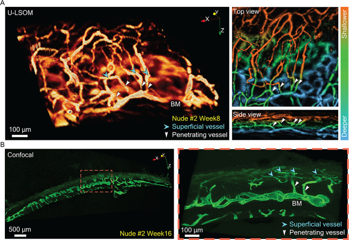
Validation of skull vasculature imaged with U‐LSOM against confocal microscopy. (A) A subregion from a U‐LSOM image of skull vasculature around the coronal suture (1 × 1 × 1 mm³ FOV). Cyan arrowheads indicate superficial vessels, and white arrowheads indicate vessels penetrating into BM compartments. Top and side views of the 3D volume are shown as depth‐encoded MIPs. (B) Confocal microscopy images of a 150‐μm‐thick skull slice around the coronal suture. Cyan arrowheads indicate superficial skull vessels, and white arrowheads indicate skull vessels penetrating into BM compartments.

Confocal imaging of skull slices

After the last time point of in vivo U‐LSOM imaging, mice were euthanized and their entire skull bone extracted and sliced as described.^{( 27 )} Consecutive slices of 150 μm thickness were generated throughout the entire bone. For confocal imaging, slices covering or proximal to the coronal suture were selected. For immunostaining, individual slices were first incubated in blocking solution (0.2% Triton X‐100, 10% donkey serum in PBS) overnight at 4°C and then stained with primary antibodies (Endomucin, 1:100; Santa Cruz Biotechnology, Santa Cruz, CA, USA; Sc‐65495) in blocking solution for 3 days at 4°C. Tissues were then washed in 0.2% Triton‐X‐100/PBS and stained with secondary antibodies (Alexa Fluor 488 donkey anti‐rat immunoglobulin G [IgG] Antibody, 1:400; Thermo Fisher Scientific, Waltham, MA, USA; A‐21208) for another 3 days at 4°C in blocking solution. Immunostained slices were washed in 0.2% Triton‐X‐100/PBS overnight and incubated in RapiClear 1.52 for 12 to 16 hours. Confocal microscopy was performed with a 10× objective (HCX PL FLUOTAR; Leica, Wetzlar, Germany) on a Leica SP8 Leica confocal microscope. Image stacks (x: 3070–3080 μm, y: 9300–10300 μm, z: 125–145 μm) were acquired with a pixel size of 2.27 μm and a Z‐step size of 3 μm. Imaris software (Oxford Instruments plc, Abingdon, UK) was used to render confocal image stacks into 3D reconstructions (Fig. 3B ).

Statistical analysis

Median and interquartile range are presented in the box plots, with median indicated as the line inside the boxes and interquartile range indicated as the length of boxes. When comparing longitudinal data, test methods for repeated measurement were considered first (Supplementary Fig. 1). If the sample distribution passed the Shapiro‐Wilk normality test, paired t test was used to calculate the p values (implemented as ttest function in MATLAB). Otherwise, the nonparametric Wilcoxon signed rank test was used (implemented as signrank function in MATLAB). Unpaired data (non‐longitudinal, e.g., comparison between different strains) also underwent normality test first. If it failed, the nonparametric Kruskal‐Wallis test was performed first (implemented as kruskalwallis function in MATLAB) to verify if any difference exists. If so, the Wilcoxon rank sum test was subsequently performed (implemented as ranksum function in MATLAB). If normality test was successful, the data would further undergo two‐sample F test for equal variance check (implemented as vartest2 function in MATLAB). If equal‐variance test was successful, two‐sample t test was used (implemented as ttest2 function in MATLAB). Otherwise, unequal variance t test was used (implemented as ttest2 function in MATLAB, with vartype parameter set to unequal). All p values, obtained from the above significance test methods, further underwent multiple testing adjustment to correct for the false discovery rate^{( 28 )} using the Benjamini and Hochberg method.^{( 29 )} A p <0.05 was considered statistically significant, and p <0.001 was considered statistically highly significant.

Results

U‐LSOM resolves intricate skull microvascular patterns in vivo

Large‐scale OA microscopy (LSOM) reveals optical absorption of hemoglobin via acoustic detection, while pulse‐echo US delineates the skull bone surface based on its distinctive acoustic impedance.^{( 23 )} A total of 15 mice (five per strain) were imaged at four time points (4, 8, 12, and 16 weeks old, Fig. 1B ), resulting in 60 volumetric datasets. Minimally‐invasive in vivo imaging was performed following a four‐step protocol^{( 22 )} (Fig. 1C ).

The co‐registered volumetric pulse‐echo US and LSOM images allowed for a reliable segmentation between the skull vessels and brain vessels beneath the skull bone, further facilitating registration of the vessels to anatomical landmarks such as Bregma, Lambda, frontal, and parietal bones (Fig. 2A–C ). The segmented skull vessels display as an intricate reticulated network sprouting from the coronal and sagittal sutures (Fig. 2C ), consistent with previous reports.^{( 8} , ^{19 )} For a 7 × 7 mm² field‐of‐view (FOV), the pulse‐echo US scan took 30 seconds at 20 μm step size, followed by a 6.5‐minute LSOM scan at 5 μm step size. U‐LSOM thus enables fast, label‐free, high‐resolution volumetric overview of the skull bone morphology and vascularization in vivo at the whole‐calvaria scale. In addition, vessel analysis tools enable identification of vessels and quantification of vascular parameters including number and size (Fig. 2D ).

To validate the segmented skull vasculature in the U‐LSOM images, we performed confocal imaging of immunostained skull slices. A subregion of U‐LSOM image around the coronal suture (1 × 1 × 1 mm³) was selected and shown as 3D volume, as well as depth‐encoded MIPs from top and side views (Fig. 3A ). The reticulated network of superficial skull vessels (cyan arrowheads), penetrating vessels (white arrowheads), and BM sinusoids at deeper skull layers were clearly revealed by U‐LSOM. The layered vasculature was confirmed in high‐resolution confocal images (Fig. 3B ), which allowed the identification of similar vessel types, including the network of superficial vessels of smaller diameter (cyan arrowheads), and penetrating vessels (white arrowheads) connecting to deeper BM vessels with typical sinusoidal morphology and larger diameter (Fig. 3B ).

Tracking skull bone morphogenesis with US microscopy

The pulse‐echo US modality facilitates monitoring of the morphological changes of the skull bone (Fig. 4A ), clearly depicting its outer surface and heterogeneity via US signal amplitude variations (e.g., orange asterisks and dashed circles, Fig. 4A ). Different time points were registered via affine transformation to facilitate quantitative analysis of longitudinal data. Anatomical landmarks were clearly revealed, including frontal and parietal bones, Bregma and Lambda, and coronal and sagittal sutures (see Fig. 2B for detailed labeling). A gradual increase in the tortuosity of the sagittal suture (i.e., the sum of all angles divided by total length) can be observed in all three strains over time (Fig. 4A , red arrows for C57BL/6J mice) as the skull plates grow and collide against each other at the sutures. Other morphogenic processes (orange dashed circles) appear as pore‐like features emerging over time and are clearly visible around the coronal sutures intersecting at the Bregma (Fig. 4A , orange asterisks for Nude mice). Interestingly, these features stand out in the parietal bones of C57BL/6J and Nude mice, whereas they remain relatively smooth for the parietal bones of CD‐1 mice.

Fig. 4.

Longitudinal tracking of skull bone morphogenesis in three mouse strains. (A) Pulse‐echo US images are shown as MIPs along depth at four time points, delineating the outer surface of the skull. SSR maps for left and right parietal bones are shown for every mouse, visualizing heterogeneities inside the skull bone. Red arrowheads indicate an increase in the tortuosity (ie, the sum of all angles divided by total length) of the sagittal suture over time. Orange dashed circles indicate US signal amplitude variations within a subregion of the parietal bone. Scale bar = 1 mm. (B) Mean SSR statistics within the full FOV for all mice in each strain. Data points corresponding to the same mouse were connected over all time points, and each color represents an individual mouse. For CD‐1 mice, the increase in SSR from week 4 to week 8 is significant (p = 0.047). For Nude mice, the increase in SSR from week 8 to week 12 is significant (p = 0.047), and the decrease in SSR from week 12 to week 16 is significant (p = 0.047). SSR = subsurface roughness.

To characterize the complexity of structures beneath the skull's outer surface, we analyzed SSR maps for the left and right parietal bones (Fig. 4A , color images in the second row of each strain). The SSR evolution indicates a general increase in the complexity of subsurface structures within the skull, consistent for all three strains. The spatial distribution of SSR reveals more homogeneous (smaller SSR) parietal bone portions closer to the Lambda (Fig. 4A ). On the other hand, strain‐specific differences in SSR dynamics were also observed (Fig. 4B ). The mean SSR increased significantly from week 4 to week 8 for CD‐1 mice (p = 0.047), and maintained at later time points. For Nude mice, the mean SSR increased significantly from week 8 to week 12 (p = 0.047), followed by a subsequent significant decrease toward week 16 (p = 0.047). No significant change in the mean SSR was found for C57BL/6J mice.

Tracking skull vessel development with LSOM

Morphological changes of skull vessels over time were revealed by segmented LSOM images (Fig. 5, first row for each strain). Although brain vessel morphology remained largely unaltered, skull vessels remodeled vastly at each time point. Skull vessels are typically found in large amounts near the sutures, especially the coronal sutures, gradually sprouting into the parietal bones at later time points. Despite the changes in skull vessel morphology over time, it is possible to track individual vessels throughout the observation period based on their distinct location and shape (Fig. 5, green‐labeled vessels).

Fig. 5.

Longitudinal tracking of skull vessel development in three mouse strains. All images are shown as MIPs along depth, with skull vessels (orange) overlaid onto brain vessels (gray). For each strain, large‐scale images are shown in the first row covering a 7 × 7 mm² FOV, and zoom‐in images covering a reduced 1.5 × 2.5 mm² FOV (labeled by a white rectangle) are shown in the second row. Selected skull vessels with distinct shape and location were tracked over time for each strain (labeled with green color). Coronal suture location is further indicated. Cyan arrows point at disappearing/reoccurring small vessels. Red arrows point at consolidating/remodeling vessels.

Zoomed‐in images at the sites of dense skull vascular network (Fig. 5, second row for each strain) further enabled quantitative statistical analysis to reveal strain‐specific differences in skull development dynamics. For C57BL/6J mice, smaller vessels mostly disappeared (cyan arrows) from week 4 to week 8. A clear difference can be observed in both CD‐1 (cyan arrows) and Nude (cyan arrows) mice during the same period—smaller vessels flourished around the tracked vessels expanding into previously unoccupied skull areas. This difference is supported by the significant increase in the total number of skull vessels from week 4 to week 8 for CD‐1 mice (p = 0.023, Fig. 6A ). Although this increase is not considered significant for Nude mice (p = 0.065), the corresponding effect size of 1.8, calculated as Cohen's d for paired samples, is considered large,^{( 30 )} which indicates a difference in the total number of skull vessels from week 4 to week 8. For C57BL/6J mice, no significant change in the total number of skull vessels was found between week 4 and week 8 (p = 0.883, effect size = 0.2). Further confirmation can be found in the distribution of skull vessel diameters (Fig. 6B ), where the number of smaller vessels (15–25 μm in diameter) peaks at week 8 for CD‐1 and Nude mice, which is not the case for C57BL/6J mice. Such observation on the vessel diameter distribution is corroborated by statistical comparison of the change in the number of newborn/small skull vessels (15–25 μm in diameter) among strains (Fig. 6C ). Compared to C57BL/6J mice, the increase in the number of small skull vessels from week 4 to week 8 is highly significant for CD‐1 (p < 0.001) and Nude (p < 0.001) mice. The imaging data and statistical analysis suggest that skull angiogenesis occurs between week 4 and week 8 for CD‐1 and Nude mice and prior to week 4 for C57BL/6J mice. From week 8 to week 12, smaller vessels around the tracked vessels mostly vanished in CD‐1 and Nude mice (zoomed‐in images in Fig. 5), similar to the observations of C57BL/6J mice from week 4 to week 8. From week 12 to week 16, skull vessels mostly remodeled and consolidated for CD‐1 and Nude mice (examples of consolidated vessels are indicated by red arrows in zoomed‐in images in Fig. 5), which is supported by preservation of the total number of skull vessels (Fig. 6A ) and a population shift to larger skull vessel diameters (Fig. 6B ). For C57BL/6J mice, skull vessels enter the remodeling and consolidation phase at an earlier time point (week 8, red arrows in zoomed‐in images in Fig. 5), which is alternatively evinced by the preservation of total number of skull vessels (Fig. 6A ) and the overlapping vessel diameter distribution (Fig. 6B ).

Fig. 6.

Quantification and statistical analysis of skull vessel parameters. (A) Total number of skull vessels for all mice in each strain. Data points corresponding to the same mouse were connected over all time points, and each color represents an individual mouse. For CD‐1 mice, the increase in total number of skull vessels from week 4 to week 8 is significant (p = 0.023). (B) Diameter distributions of all skull vessels for all mice in each strain. (C) Statistical comparison of the changes in the number of newborn/small skull vessels (15–25 μm in diameter) among strains and between time points. From week 4 to week 8, p = 0.0005 (C57BL/6J versus CD‐1) and p = 0.0005 (C57BL/6J versus Nude). From week 12 to week 16, p = 0.004 (CD‐1 versus C57BL/6J) and p = 0.008 (CD‐1 versus Nude).

Monitoring the coupling of angiogenesis and osteogenesis

The interplay between morphological changes of skull bone and its vascular network can be assessed based on the combined pulse‐echo US and LSOM information provided by U‐LSOM. Longitudinal changes in skull bone thickness and vessel fill fraction were quantified by selecting six different ROIs for each strain (Fig. 7). Skull bone thickness was estimated based on the depth‐matched information in the volumetric US and LSOM images, whereas vessel fill fraction was calculated as percentage of the ROI covered by skull vessels. From week 4 to week 8, as smaller vessels appear in the surroundings of the tracked vessels in CD‐1 and Nude mice, a corresponding significant increase in vessel fill fraction can be observed (p = 0.005 for CD‐1 mice, p = 0.018 for Nude mice). The highly significant increase in skull bone thickness occurred at a later time point (ie, week 12) for CD‐1 (p < 0.001) and Nude (p < 0.001) mice, accompanied by insignificant changes in vessel fill fraction from week 8 to week 12. In contrast, the highly significant increase in skull thickness occurred from week 4 to week 8 for C57BL/6J mice (p < 0.001), accompanied by significant reduction in vessel fill fraction (p = 0.005). This observation confirms the above postulate that skull angiogenesis takes place at different timeframe in different strains, namely, week 4 to week 8 for CD‐1 and Nude mice, and prior to week 4 for C57BL/6J mice. The above longitudinal analysis on skull thickness and vessel fill fraction thus supports the general observation of angiogenesis being a precursor of osteogenesis.

Fig. 7.

Coupling between angiogenesis and osteogenesis revealed by U‐LSOM. Longitudinal analysis of the coupling between angiogenesis (increase in vessel fill fraction) and osteogenesis (increase in skull bone thickness). Six different regions‐of‐interest were selected and quantified for each strain. For C57BL/6J mice, the fill fraction decrease is significant from week 4 to week 8 (p = 0.005), and the increase in thickness is highly significant (p = 0.00002). From week 8 to week 12, the increase in thickness is significant (p = 0.004). For CD‐1 mice, the increase in fill fraction is significant from week 4 to week 8 (p = 0.005). The increase in thickness is significant from week 4 to week 8 (p = 0.005), and highly significant from week 8 to week 12 (p = 0.0002). For Nude mice, the increase in fill fraction is significant from week 4 to week 8 (p = 0.018). The increase in thickness is significant from week 4 to week 8 (p = 0.031), and highly significant from week 8 to week 12 (p = 0.0005).

Discussion

In this study, we used U‐LSOM to visualize developing vasculature over frontal, bregma, and parietal areas of murine calvaria. The rapid scanning procedure enabled high‐throughput imaging at the whole‐calvaria scale, thus overcoming longstanding limitations of multiphoton microscopy and other classical intravital optical techniques that may require several hours to acquire volumetric FOVs of comparable size.^{( 10} , ³¹ , ^{32 )} μCT finds its strength in evaluating detailed anatomical features and quantifying bone volume changes over time, albeit the high X‐ray radiation exposure and limited contrast hinder its applicability in long‐term in vivo studies.^{( 27 )} On the other hand, by means of the quantitative automatic vessel segmentation and analysis algorithm, large‐scale morphology of the skull microvasculature and skeletal system can be monitored and analyzed by U‐LSOM in vivo with a spatial resolution better than 10 μm.^{( 24 )} Therefore, U‐LSOM may provide complementary information to μCT interrogations, enabling quantitative evaluation of skull bone development and repair dynamics. Additionally, the noninvasivity of U‐LSOM provides a safe and robust in vivo imaging platform for longitudinal studies of developing calvaria in the same animal over time. This offers significant advantages over ex vivo imaging approaches where different developmental stages are studied in different animals, such as light‐sheet fluorescence microscopy^{( 32 )} that involves additional optical clearing of bones for rendering calvarian vasculature in 3D.

Osteogenesis in three common mouse strains (C57BL/6J, CD‐1 and Nude) was monitored and compared based on skull roughness and thickness. Similarly, angiogenesis was evaluated by tracking specific vessels and their surrounding vascular morphology changes over time. The relations between skull vessel fill fraction and skull bone thickness revealed a temporal delay between the skull bone and vessel growth, consistent with previous observations.^{( 4} , ^{33 )} To the best of our knowledge, this is the first time that developmental dynamics of the skull angiogenesis and osteogenesis are monitored simultaneously at the whole‐calvaria scale in vivo in a label‐free manner. Note that immunostaining and confocal microscopy of skull slices were performed after the last imaging time point as a validation against U‐LSOM. The evolution of skull SSR from week 4 to week 8 across the strains was consistent with their corresponding angiogenesis progression, which might be ascribed to the newborn blood microvessels contributing to the increased complexity within the skull bone.

Not only skull angiogenesis but also vascular remodeling was observed over a 3‐month period by employing a minimally‐invasive temporary scalp‐opening procedure. The quantitative vessel analysis results were in line with previous studies showing that vascular growth is largely concluded at 8 weeks of age.^{( 3} , ^{34 )} It is also discernible that certain skull vessels started to merge and reshape at later time points (12 and 16 weeks), suggesting that vascular remodeling was underway to potentially establish local blood supply in surrounding BM.^{( 3 )}

Strain‐specific differences in skull vessel growth patterns were observed. Compared to CD‐1 and Nude mice, plenty of smaller skull vessels were already observed in 4‐week‐old C57BL/6J mice, suggesting that vasculogenesis and angiogenesis commence at an earlier time point. On the other hand, the trend of total number of vessels suggests that CD‐1 and Nude mice enter the vascular remodeling phase starting at week 12. The vessel growth and remodeling processes can alternatively be observed by assessing distribution of the skull vessel diameter, which shifted toward larger diameters over time, in agreement with previous findings.^{( 35 )}

We compared in vivo volumetric U‐LSOM images with ex vivo confocal images of skull slices to identify vascular features related to BM. The latter is known to regulate oxygen levels and nutrient supply to maintain hematopoietic function, and is used by de novo produced hematopoietic stem cells (HSCs) to access systemic circulation. Endothelial cells lining BM vessels further create crucial perivascular niches for HSC maintenance and preservation of mesenchymal osteoprogenitor cells involved in bone metabolism.^{( 36} , ^{37 )} Furthermore, recently described transcortical vascular channels connect marrow tissues with brain parenchyma and are used by myeloid cells to directly access BM‐derived myeloid cells during local inflammatory reactions.^{( 31} , ^{38 )} Thus, the use of intravital imaging techniques to study the vascular networks connecting bone, BM, and brain, and their dynamic remodeling over time, may contribute to our understanding of the complex local interplay between these organs. In U‐LSOM images, a reticulated superficial vascular network is clearly seen to connect to arterial vessels penetrating into BM compartments, which was confirmed by confocal microscopy. The observation of these transcalvarial vessels connecting BM and its outer environment further demonstrates the potential of U‐LSOM for future studies on BM perfusion in health and disease.

Hypoxia is one of the niche characteristics to maintain quiescence in multiple stem cell types in the BM. Thus, quantification of local oxygen concentration could provide unique information about vascular density and oxygen supply/consumption in the skull.^{( 39 )} To this end, different OA microscopy embodiments have been shown capable of providing information on oxygen saturation (sO₂) in the mouse brain.^{( 40 )} Extending the U‐LSOM to multiple wavelengths would enable sO₂ imaging, thus help investigating hypoxic conditions in different skull regions.^{( 41 )} In addition, sO₂ information could potentially facilitate efficient discrimination between arteries and veins. Blood flow patterns could also aid in differentiating skull vessel subtypes in the BM microvasculature.^{( 7} , ^{36 )} Previous studies measured the flow velocities of individual arteries and sinusoids to understand the hematopoietic stem/progenitor cell homing and microcirculation in the BM niches, enabled by various vascular markers.^{( 7} , ^{36 )} OA imaging has also been shown to image blood flow in vivo.^{( 42 )} Likewise, the U‐LSOM analysis could be extended to further enable the identification of skull vessel subtypes. Moreover, multimodal imaging would be a powerful tool to understand the dynamics of BM cells, vascularization, and bone formation.^{( 6} , ^{43 )} Other widefield optical microscopy techniques could be integrated into the dual‐modal U‐LSOM to provide complementary information on, e.g., blood flow.^{( 44 )}

Prolonged isoflurane anesthesia is associated with a significant increase in brain water content, leading to edema formation.^{( 45 )} The segmentation of skull and brain vessels was thus less effective at 4 weeks of age compared to later time points, which might be attributed to the reduced skull thickness with some brain vessels located very close to the skull inner surface due to brain edema. A triple anesthesia mixture of midazolam, medetomidine, and fentanyl could potentially prevent the brain swelling and improve segmentation quality for 4‐week‐old mice.

The current study design included an “I”‐shaped cut for opening the scalp every 4 weeks to monitor skull vessel development patterns in the same mice longitudinally. Although a 4‐week period is enough for the cut to heal in principle, it is still possible that a scar was forming and led to a degraded image quality. Thus, a “C” or “L”‐shaped cut could be performed in future experiments to ensure an intact central region of the skull.^{( 46 )} Alternatively, a calvarial window model, where a thin cover glass is attached onto the mouse calvaria, could be implemented for the longitudinal study,^{( 47 )} in which case the mouse only needs to undergo a single surgery in the beginning of the study.

It is widely acknowledged that blood supply plays a key role in bone growth and regeneration.^{( 2} , ⁴ , ^{5 )} Previous studies used mouse models of bone defect healing to evaluate angiogenesis during bone repair,^{( 35 )} and explore the mechanisms of osteoprogenitor cell interactions with bone healing microenvironment.^{( 33 )} U‐LSOM is well suited to conduct longitudinal studies on the healing of such defects by assessing vessel/bone morphology alternations with high spatial resolution and penetration depth. Specifically, parameters like vessel diameter and density and the defected skull area could be directly quantified in a label‐free manner.

U‐LSOM not only finds applicability in studies on fracture healing, but may also benefit studies on musculoskeletal tumors. Osseous hemangioma (venous vascular malformation) is one kind of musculoskeletal tumors characterized by vascular lesions in bone and soft tissue.^{( 48} , ^{49 )} Most such vascular tumors in the skull contain dilated blood vessels separated by fibrous septa with serpentine vascular channels lesions,^{( 49 )} whose vascularization parameters can be monitored with U‐LSOM over a long term. U‐LSOM thus provides a high‐throughput platform for studying the interconnection and long‐term dynamics of skull bone and brain vasculature, meningeal lymphatic vessels,^{( 50 )} and cerebrospinal fluid pathways^{( 51 )} upon injection of contrast agents.

In summary, we used U‐LSOM to longitudinally monitor the growth pattern of skull vessels and bones at different developmental stages in mice. Strain‐specific differences in angiogenesis and vascular remodeling timeframe were observed. The label‐free, minimally‐invasive observation of vascular and bone morphology is crucial to understand skull growth at the whole‐brain scale. The established imaging platform opens up new possibilities for high‐throughput, long‐term, minimally‐invasive preclinical studies on the critical link between blood vessel formation, and skull bone growth and regeneration in vivo.

Author Contributions

Weiye Li: Data curation; formal analysis; investigation; methodology; project administration; resources; software; validation; visualization; writing – original draft; writing – review and editing. Yu‐Hang Liu: Data curation; formal analysis; investigation; methodology; project administration; resources; software; validation; visualization; writing – original draft; writing – review and editing. Hector Estrada: Conceptualization; investigation; methodology; project administration; resources; software; supervision; validation; visualization; writing – original draft; writing – review and editing. Johannes Rebling: Conceptualization; investigation; methodology; project administration; resources; software; supervision; validation; visualization; writing – original draft; writing – review and editing. Michael Reiss: Data curation; investigation; methodology; resources; visualization; writing – review and editing. Serena Galli: Data curation; formal analysis; investigation; methodology; resources; validation; visualization; writing – review and editing. César Nombela‐Arrieta: Formal analysis; investigation; methodology; project administration; supervision; validation; writing – review and editing. Daniel Razansky: Conceptualization; formal analysis; funding acquisition; investigation; methodology; project administration; resources; supervision; writing – original draft; writing – review and editing.

Disclosures

All authors state that they have no conflicts of interest.

Peer Review

The peer review history for this article is available at https://publons.com/publon/10.1002/jbmr.4533.

Supporting information

Supplementary Fig. 1 Flowchart illustrating selection of the statistical significance test methods.

Data Availability Statement

The data that support the findings of this study are available from the corresponding author upon reasonable request.

References

- 1. Gerber HP, Ferrara N. Angiogenesis and bone growth. Trends Cardiovasc Med. 2000;10(5):223‐228. [DOI] [PubMed] [Google Scholar]
- 2. Kusumbe AP, Ramasamy SK, Adams RH. Coupling of angiogenesis and osteogenesis by a specific vessel subtype in bone. Nature. 2014;507(7492):323‐328. [DOI] [PMC free article] [PubMed] [Google Scholar]
- 3. Sivaraj KK, Adams RH. Blood vessel formation and function in bone. Development. 2016;143(2715):2706‐2715. [DOI] [PubMed] [Google Scholar]
- 4. Carano RAD, Filvaroff EH. Angiogenesis and bone repair. Drug Discov Today. 2003;8(21):980‐989. [DOI] [PubMed] [Google Scholar]
- 5. Hankenson KD, Dishowitz M, Gray C, Schenker M. Angiogenesis in bone regeneration. Injury. 2011;42(6):556‐561. [DOI] [PMC free article] [PubMed] [Google Scholar]
- 6. Lassailly F, Foster K, Lopez‐Onieva L, Currie E, Bonnet D. Multimodal imaging reveals structural and functional heterogeneity in different bone marrow compartments: functional implications on hematopoietic stem cells. Blood. 2013;122(10):1730‐1740. [DOI] [PubMed] [Google Scholar]
- 7. Bixel MG, Kusumbe AP, Ramasamy SK, et al. Flow dynamics and HSPC homing in bone marrow microvessels. Cell Rep. 2017;18(7):1804‐1816. [DOI] [PMC free article] [PubMed] [Google Scholar]
- 8. Toriumi H, Shimizu T, Shibata M, et al. Developmental and circulatory profile of the diploic veins. Microvasc Res. 2011;81(1):97‐102. [DOI] [PubMed] [Google Scholar]
- 9. Mazo IB, Gutierrez‐Ramos J‐C, Frenette PS, et al. Hematopoietic progenitor cell rolling in bone marrow microvessels: parallel contributions by endothelial selectins and vascular cell adhesion molecule 1. J Exp Med. 1998;188(3):465‐474. [DOI] [PMC free article] [PubMed] [Google Scholar]
- 10. Ahn S, Choe K, Lee S, et al. Intravital longitudinal wide‐area imaging of dynamic bone marrow engraftment and multilineage differentiation through nuclear‐cytoplasmic labeling. PLoS One. 2017;12(11):1‐16. [DOI] [PMC free article] [PubMed] [Google Scholar]
- 11. Baltes C, Radzwill N, Bosshard S, Marek D, Rudin M. Micro MRI of the mouse brain using a novel 400 MHz cryogenic quadrature RF probe. NMR Biomed. 2009;22(8):834‐842. [DOI] [PubMed] [Google Scholar]
- 12. Starosolski Z, Villamizar CA, Rendon D, et al. Ultra high‐resolution in vivo computed tomography imaging of mouse cerebrovasculature using a long circulating blood Pool contrast agent. Sci Rep. 2015;5(1):10178. [DOI] [PMC free article] [PubMed] [Google Scholar]
- 13. Sipkins DA, Wei X, Wu JW, et al. In vivo imaging of specialized bone marrow endothelial microdomains for tumour engraftment. Nature. 2005;435(7044):969‐973. [DOI] [PMC free article] [PubMed] [Google Scholar]
- 14. Kim JM, Bixel MG. Intravital multiphoton imaging of the bone and bone marrow environment. Cytometry A. 2020;97(5):496‐503. [DOI] [PubMed] [Google Scholar]
- 15. Beard P. Biomedical photoacoustic imaging. Interface Focus. 2011;1(4):602‐631. [DOI] [PMC free article] [PubMed] [Google Scholar]
- 16. Wang LV, Yao J. A practical guide to photoacoustic tomography in the life sciences. Nat Methods. 2016;13(8):627‐638. [DOI] [PMC free article] [PubMed] [Google Scholar]
- 17. Ning B, Sun N, Cao R, et al. Ultrasound‐aided multi‐parametric photoacoustic microscopy of the mouse brain. Sci Rep. 2015;5:18775. [DOI] [PMC free article] [PubMed] [Google Scholar]
- 18. Rebling J, Estrada H, Gottschalk S, et al. Dual‐wavelength hybrid optoacoustic‐ultrasound biomicroscopy for functional imaging of large‐scale cerebral vascular networks. J Biophotonics. 2018;11(9):e201800057. [DOI] [PubMed] [Google Scholar]
- 19. Estrada H, Rebling J, Sievert W, et al. Intravital optoacoustic and ultrasound bio‐microscopy reveal radiation‐inhibited skull angiogenesis. Bone. 2020;133:115251. [DOI] [PubMed] [Google Scholar]
- 20. Zhao Q, Lin R, Liu C, et al. Quantitative analysis on in vivo tumor‐microvascular images from optical‐resolution photoacoustic microscopy. J Biophotonics. 2019;12(6):1‐15. [DOI] [PubMed] [Google Scholar]
- 21. Zhou HC, Chen N, Zhao H, et al. Optical‐resolution photoacoustic microscopy for monitoring vascular normalization during anti‐angiogenic therapy. Photoacoustics. 2019;15:100143. [DOI] [PMC free article] [PubMed] [Google Scholar]
- 22. Wu JW, Runnels JM, Lin CP. Intravital imaging of hematopoietic stem cells in the mouse skull. Methods Mol Biol. 2014;1185:247‐265. [DOI] [PubMed] [Google Scholar]
- 23. Estrada H, Rebling J, Hofmann U, Razansky D. Discerning calvarian microvascular networks by combined optoacoustic ultrasound microscopy. Photoacoustics. 2020;19:100178. [DOI] [PMC free article] [PubMed] [Google Scholar]
- 24. Rebling J, Ben‐Yehuda Greenwald M, Wietecha M, Werner S, Razansky D. Long‐term imaging of wound angiogenesis with large scale optoacoustic microscopy. Adv Sci. 2021;8(13):2004226. [DOI] [PMC free article] [PubMed] [Google Scholar]
- 25. razanskylab/PostProGUI [Internet]. Available from: https://github.com/razanskylab/PostProGUI.
- 26. joe‐of‐all‐trades/vtkwrite [Internet]. Available from: https://github.com/joe-of-all-trades/vtkwrite.
- 27. Dall'Ara E, Boudiffa M, Taylor C, et al. Longitudinal imaging of the ageing mouse. Mech Ageing Dev. 2016;160:93‐116. [DOI] [PubMed] [Google Scholar]
- 28. Storey JD, Tibshirani R. Statistical significance for genomewide studies. Proc Natl Acad Sci U S A. 2003;100(16):9440‐9445. [DOI] [PMC free article] [PubMed] [Google Scholar]
- 29. Benjamini Y, Hochberg Y. Controlling the false discovery rate: a practical and powerful approach to multiple testing. J R Stat Soc Ser B. 1995;57(1):289‐300. [Google Scholar]
- 30. Cohen J. The t test for means. Statistical Power Analysis for the Behavioral Sciences. New York, NY: Elsevier; 1977. pp 19‐74. [Google Scholar]
- 31. Herisson F, Frodermann V, Courties G, et al. Direct vascular channels connect skull bone marrow and the brain surface enabling myeloid cell migration. Nat Neurosci. 2018;21(9):1209‐1217. [DOI] [PMC free article] [PubMed] [Google Scholar]
- 32. Grüneboom A, Hawwari I, Weidner D, et al. A network of trans‐cortical capillaries as mainstay for blood circulation in long bones. Nat Metab. 2019;1(2):236‐250. [DOI] [PMC free article] [PubMed] [Google Scholar]
- 33. Huang C, Ness VP, Yang X, et al. Spatiotemporal analyses of osteogenesis and angiogenesis via Intravital imaging in cranial bone defect repair. J Bone Miner Res. 2015;30(7):1217‐1230. [DOI] [PMC free article] [PubMed] [Google Scholar]
- 34. Maes C, Kobayashi T, Selig MK, et al. Osteoblast precursors, but not mature osteoblasts, move into developing and fractured bones along with invading blood vessels. Dev Cell. 2010;19(2):329‐344. [DOI] [PMC free article] [PubMed] [Google Scholar]
- 35. Holstein JH, Becker SC, Fiedler M, et al. Intravital microscopic studies of angiogenesis during bone defect healing in mice calvaria. Injury. 2011;42(8):765‐771. [DOI] [PubMed] [Google Scholar]
- 36. Morikawa T, Tamaki S, Fujita S, Suematsu M, Takubo K. Identification and local manipulation of bone marrow vasculature during intravital imaging. Sci Rep. 2020;10(1):1‐10. [DOI] [PMC free article] [PubMed] [Google Scholar]
- 37. Nombela‐Arrieta C, Manz MG. Quantification and three‐dimensional microanatomical organization of the bone marrow. Blood Adv. 2017;1(6):407‐416. [DOI] [PMC free article] [PubMed] [Google Scholar]
- 38. Cugurra A, Mamuladze T, Rustenhoven J, et al. Skull and vertebral bone marrow are myeloid cell reservoirs for the meninges and CNS parenchyma. Science. 2021;373:eabf7844. [DOI] [PMC free article] [PubMed] [Google Scholar]
- 39. Spencer JA, Ferraro F, Roussakis E, et al. Direct measurement of local oxygen concentration in the bone marrow of live animals. Nature. 2014;508(7495):269‐273. [DOI] [PMC free article] [PubMed] [Google Scholar]
- 40. Yao J, Wang L, Yang JM, et al. High‐speed label‐free functional photoacoustic microscopy of mouse brain in action. Nat Methods. 2015;12(5):407‐410. [DOI] [PMC free article] [PubMed] [Google Scholar]
- 41. Liu C, Liang Y, Wang L. Single‐shot photoacoustic microscopy of hemoglobin concentration, oxygen saturation, and blood flow in sub‐microseconds. Photoacoustics. 2020;17:100156. [DOI] [PMC free article] [PubMed] [Google Scholar]
- 42. van den Berg PJ, Daoudi K, Steenbergen W. Review of photoacoustic flow imaging: its current state and its promises. Photoacoustics. 2015;3(3):89‐99. [DOI] [PMC free article] [PubMed] [Google Scholar]
- 43. Mendez A, Rindone AN, Batra N, et al. Phenotyping the microvasculature in critical‐sized calvarial defects via multimodal optical imaging. Tissue Eng Part C Methods. 2018;24(7):430‐440. [DOI] [PMC free article] [PubMed] [Google Scholar]
- 44. Chen Z, Zhou Q, Rebling J, Razansky D. Cortex‐wide microcirculation mapping with ultrafast large‐field multifocal illumination microscopy. J Biophotonics. 2020;13(11):1‐7. [DOI] [PubMed] [Google Scholar]
- 45. Stover JF, Kroppenstedt SN, Thomale UW, Kempski OS, Unterberg AW. Isoflurane doubles plasma glutamate and increases posttraumatic brain edema. Brain Edema XI: Proceedings of the 11th International Symposium, Newcastle‐upon‐Tyne, United Kingdom, June 6–10, 1999. Vienna: Springer; 2000. pp 375‐378. [DOI] [PubMed] [Google Scholar]
- 46. Lo Celso C, Lin CP, Scadden DT. In vivo imaging of transplanted hematopoietic stem and progenitor cells in mouse calvarium bone marrow. Nat Protoc. 2011;6(1):1‐14. [DOI] [PMC free article] [PubMed] [Google Scholar]
- 47. Le VH, Lee S, Lee S, et al. In vivo longitudinal visualization of bone marrow engraftment process in mouse calvaria using two‐photon microscopy. Sci Rep. 2017;7:44097. [DOI] [PMC free article] [PubMed] [Google Scholar]
- 48. Lloret I, Server A, Taksdal I. Calvarial lesions: a radiological approach to diagnosis. Acta Radiol. 2009;50(5):531‐542. [DOI] [PubMed] [Google Scholar]
- 49. Gomez CK, Schiffman SR, Bhatt AA. Radiological review of skull lesions. Insights Imaging. 2018;9(5):857‐882. [DOI] [PMC free article] [PubMed] [Google Scholar]
- 50. Ahn JH, Cho H, Kim JH, et al. Meningeal lymphatic vessels at the skull base drain cerebrospinal fluid. Nature. 2019;572:62‐66. [DOI] [PubMed] [Google Scholar]
- 51. Mestre H, Du T, Sweeney AM, et al. Cerebrospinal fluid influx drives acute ischemic tissue swelling. Science. 2020;367:eaax7171. [DOI] [PMC free article] [PubMed] [Google Scholar]
Associated Data
This section collects any data citations, data availability statements, or supplementary materials included in this article.
Supplementary Materials