Report on the AAPM deep-learning sparse-view CT (DL-sparse-view CT) Grand Challenge

Abstract

Purpose:

The purpose of the challenge is to find the deep-learning technique for sparse-view CT image reconstruction that can yield the minimum RMSE under ideal conditions, thereby addressing the question of whether or not deep learning can solve inverse problems in imaging.

Methods:

The challenge set-up involves a 2D breast CT simulation, where the simulated breast phantom has random fibro-glandular structure and high-contrast specks. The phantom allows for arbitrarily large training sets to be generated with perfectly known truth. The training set consists of 4000 cases where each case consists of the truth image, 128-view sinogram data, and the corresponding 128-view filtered back-projection (FBP) image. The networks are trained to predict the truth image from either the sinogram or FBP data. Geometry information is not provided. The participating algorithms are tested on a data set consisting of 100 new cases.

Results:

About 60 groups participated in the challenge at the validation phase, and 25 groups submitted test-phase results along with reports on their deep-learning methodology. The winning team improved reconstruction accuracy by two orders of magnitude over our previous CNN-based study on a similar test problem.

Conclusions:

The DL-sparse-view challenge provides a unique opportunity to examine the state-of-the-art in deep-learning techniques for solving the sparse-view CT inverse problem.

I. Introduction

The American Association of Physics in Medicine (AAPM) sponsored a recent Grand Challenge that addresses the use of deep-learning (DL) and convolutional neural networks (CNNs) for solving the inverse problem associated with sparse-view computed tomography (CT) image reconstruction^1,2,3. The challenge began on March 17th 2021, when the training data became available, and it concluded on June 1st 2021, the last day for submission of test results. During the challenge there were approximately 60 teams that were actively participating and around 500 trial submissions were made. In the final test phase, 25 team submitted their image predictions along with a report on their DL methodology. This article presents the background and results of the challenge along with an analysis on what we have learned about the use of DL for solving inverse problems in tomographic imaging.

The idea for the challenge started from claims made in the literature that CNNs can solve inverse problems that arise in CT image reconstruction^4,5,6. In response to those claims, we performed a study along with Lorente and Brankov⁷, where we investigated the question of whether or not CNNs can solve the inverse problem associated with sparse-view CT image reconstruction. In our article⁷, we attempted to implement CNN-based image reconstruction based on^4,5 and we were not able to demonstrate that CNNs can solve the sparse-view CT problem. The conclusion of our work was that there is no evidence that CNNs can solve such problems despite the claims made in the literature. We did, however, acknowledge that there may be other DL-based image reconstruction algorithms that are capable of inverting the sparse-view CT model.

Carrying out a broad survey of DL-based methods for CT image reconstruction, is the motivation for the DL-sparse-view CT challenge. In effect the challenge is a “crowd-source” effort where researchers could apply their own DL technology on a well-defined sparse-view CT problem. The goal of the challenge is accurate recovery of the test images from ideal noiseless projection data; accordingly algorithms can be ranked unambiguously with root-mean-square-error (RMSE) and the floor of this metric is zero at which point one can say that the CT inverse problem is solved.

We are happy to report that the participation and the ingenuity of the developed DL-based algorithms greatly exceeded our expectations. The winning team of DL-sparse-view CT challenge report a RMSE score – two orders of magnitude smaller than what was reported for the DL-based method in Sidky et al.⁷ for a similar image reconstruction set-up. Furthermore, there is a healthy spread of scores resulting from the numerous DL-based implementations employed. As such, it is possible to start to gauge the success of various DL designs for CT image reconstruction.

In Sec. II. the details of the DL-sparse-view CT challenge are outlined, discussing the problem set-up, evaluation metrics, and challenge logistics. In Sec III., the results of the challenge are presented, including statistics of all scores along with groupings of scores according to the general class of DL methodology and a focus on the results of the top five participating teams. Section IV. discusses how the results relate to the question of solving the CT inverse problem and concludes the paper.

II. Methods

II.A. Inverse problem theory

The motivation for the DL sparse-view CT challange is the investigation of the inverse problem associated with sparse-view CT image reconstruction, and accordingly we provide a brief review of inverse problem theory. At a high level, inverse problems require the specification of a measurement model⁸

$$y=\mathcal{M}(x),$$

where x represents unknown model parameters; and $\mathcal{M}$ is an operator that yields the data y from x. For deriving inverses, this measurement model usually represents a simplified physical model, which is on the one hand complex enough to capture the dominant physics of the imaging problem but simple enough that deriving an inverse is a tractable mathematical problem. For the sparse-view CT problem of interest, x is a discrete CT image; $\mathcal{M}$ represents discrete-to-discrete linear forward projection; and y is the sparsely sampled sinogram. Solving the inverse problem entails deriving ${\mathcal{M}}^{-1}$ such that

$$x={\mathcal{M}}^{-1}(y).$$

Solving an inverse problem is a binary issue; either test images are recovered exactly for this model or they are not.

Inverse problem studies confer generalizability to a proposed model inversion technique. Once it is established that ${\mathcal{M}}^{-1}$ inverts the measurement model, we know that any x can be recovered from data y in the range of $\mathcal{M}$. Also, generalizable stability results rely on demonstration of inverting the idealized model. A realistic, perhaps intractable model ${\mathcal{M}}_{\mathrm{phys}}$, can be written in terms of an idealized model as

$${\mathcal{M}}_{\mathrm{phys}}(x)=\mathcal{M}(x)+ϵ(x),$$

where ϵ(x) represents both deterministic and statistical model error. A stability result puts a bound on the reconstruction error ${\mathcal{M}}^{-1}(ϵ(x))$ only if ${\mathcal{M}}^{-1}$ is the true inverse of the idealized model $\mathcal{M}$.

Inverse problem studies also play a central role in the reproducability of image reconstruction algorithms. From an engineering perspective, all image reconstruction algorithms are implemented on a computer, and the more complex an algorithm is, the more difficult it is to debug. Checking that x can be recovered accurately from ideal data y in the range of $\mathcal{M}$ provides a stringent test on the computer code. If the model inverse ${\mathcal{M}}^{-1}$ is known, any error in the recovery of x must be due to implementation or numerical error. Note that applying a model inverse to noisy corrupted data will yield ambiguous results with respect to algorithm validation. There will be error in x, but it is difficult to say whether this error is due to implementation error, data error, or a combination of both.

The present DL-sparse-view CT challenge is simulation-based and it addresses the concrete issue as to whether or not a deep-learning network can solve the inverse problem of sparse-view CT image reconstruction.

II.B. Sparse-view CT simulation and object modeling

The simulation is based on breast CT and it is similar to the one used in Sidky et al..⁷ The CT data model is the standard discrete-to-discrete linear model that is commonly used in CT iterative image reconstruction

$$g=Xf,$$

where g represents the discrete sinogram data; X is a linear transform encoding X-ray projection; and f is the pixelized image array representing the scanned subject. Matching up with the inverse problem formalism, the image pixels f represent the unknown model parameters x; the measurement model $\mathcal{M}(·)$ is matrix multiplication by X; and the sinogram data g are associated with the the model measurements y. The image array is 512x512 pixels covering an area (18cm)². The line-intersection method is used for generating the matrix elements of X. The scan configuration is 2D sparse-view CT, where 128 evenly space projections are acquired over a 360 degree scan. A fan-beam configuration is used with a source-to-detector distance of 100 cm and a source-to-center-of-rotation distance of 50 cm. The linear detector array has 1024 detector elements. For the challenge image reconstruction problem, the data g are generated by applying X to test images f and the goal is to see if participants can recover f from the sinogram g. As the image size is 512² and the sinogram size is 128×1024, it is clear that the problem is under-sampled because there are more unknown pixel values than sinogram measurements.

Because the image reconstruction algorithms in question are data-driven techniques, the object modeling is the most crucial component to the simulation. The breast phantom model^7,9 is stochastic so that multiple realizations can be generated for the purpose of training, validation, and testing. Three realizations of this object model are shown in Fig. 1 along with the corresponding sinograms and filtered back-projection (FBP) images. All breast slice realizations are centered on the middle of the image area, and have a circular profile of radius 8 cm. Four tissues are modeled: adipose with an attenuation of 0.194 cm⁻¹, skin and fibroglandular tissue at 0.233 cm⁻¹, and single-pixel specks resembling microcalcifications with variable attenuation ranging from 0.333 to 0.733 cm⁻¹. The random components of the phantom are the fibroglandular morphology, the speck number (between 10 and 25 per phantom realization), speck location, and speck amplitude. The speck location is restricted to the fibroglandular regions. After generating the phantom with discrete gray levels, we apply Gaussian smoothing with a full width at half maximum of one pixel, in this way the gray levels of the phantom varies smoothly between the tissue types.

Figure 1:

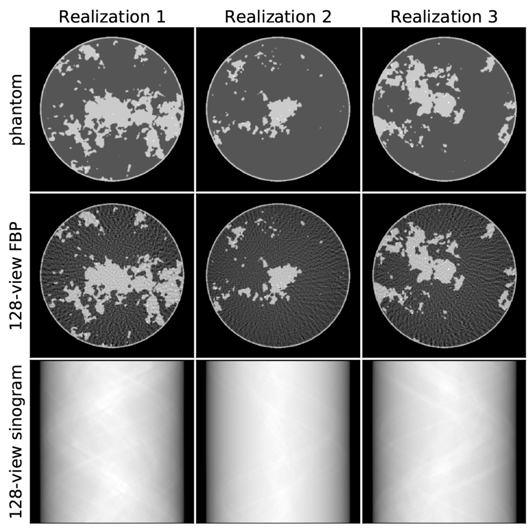
(Top row) Three realizations of the breast phantom model. (Middle row) Corresponding FBP image obtained from the 128-view sinogram (Bottom row). The images are shown in a gray scale window of [0.174,0.253] cm⁻¹.

The breast phantom images are challenging to recover mainly due to the complex fibroglandular morphology. The image smoothing and random speck amplitudes prevents hard-coding discrete gray levels or a tight upper bound for the fibroglandular component of the phantom. Despite the object complexity, it is amenable to sparsity-exploiting image reconstruction techniques because the phantom can be expressed as the gaussian blurring of an image that has a sparse spatial gradient magnitude image. In Sidky et al.⁷, accurate image reconstruction for this CT configuration and breast model is demonstrated with a standard sparsity exploiting image reconstruction technique. The purpose of designing the object so that model inversion is possible by exploiting gradient-sparsity is to demonstrate that solution of this sparse-view CT system is possible. In this way, for whatever image reconstruction technique that is developed, we know in advance that numerically exact object recovery is possible.

II.C. Challenge logistics and scoring metrics

In order to explain the information provided for this challenge, we refer to the taxonomy of DL techniques for inverse problems in imaging provided in Ongie et al..¹⁰ The DL taxonomy is organized along two axes: (1) knowledge of the system matrix, and (2) quality of the training data. Because we are interested in image recovery under ideal conditions, we provide training data of the highest quality, i.e. supervised learning with exact knowledge of the ground truth images. The DL sparse-view CT challenge focuses on the first axis of the DL taxonomy: (i) X is known exactly, (ii) X is known only at test time, (iii) X is partially known, and (iv) X is unknown. In the literature for DL-based image reconstruction for CT, by far the most common approach involves predicting the truth image from an FBP reconstructed image, using a U-net to remove the streak artifacts inherent in the latter.^4,5 This strategy falls into the first category of DL techniques because the exact geometry of the scan configuration, which specifies X, is exploited in obtaining the FBP image that serves as the input to the CNN. On the other extreme, the automated transform by manifold approximation (AUTOMAP) framework⁶ is an example of the last category; for this type of approach the transformation from sinogram to image is learned without knowledge of X or the scan geometry. There are also numerous techniques for incorporating a CNN into an iterative procedure, see Ongie et al.¹⁰ for a survey. The most common form of this approach is the unrolled iterative technique, which belongs to the first category where knowledge of X is available. In the unrolled iterative technique a finite number of iterations are performed, alternating between a regularization step and a standard data-consistency step. The CNN is used for the regularization step, and knowledge of X is exploited in the data-consistency step. Finally, standard iterative image reconstruction can be used with inexact knowledge of X, i.e. category (iii). The resulting images will have artifacts resulting from the use of an inexact system matrix X, and these artifacts can be mitigated by a U-net CNN in a similar way as is done with the FBP-CNN method.

For the DL sparse-view CT challenge, we provided 128-view FBP images, 128-view sinograms, and the knowledge that the scan geometry is a circular, fan-beam configuration. We did not provide the geometry parameters or the scheme for generating the weights of the system matrix X. Under these conditions, DL methods from category (i) had to involve the use of the 128-view FBP images. The challenge does not test category (ii) methods because we used the same X in generating the training and testing data. Category (iii) methods could be developed for the challenge by exploiting a low-parameter description of X and using the sinograms and truth images in the training set to arrive at scan parameter values for an estimate of X. Finally, the challenge also admitted category (iv) approaches which do not require X, such as AUTOMAP, or that estimate the scan geometry parameters simultaneously with the image itself. By not providing the system matrix X, the challenge barred hybrid DL/iterative appoaches in category (i). This was necessary, because the design of the image reconstruction problem is such that it can be solved by constrained, TV-minimization with the smoothed-object model.⁷ With knowledge of X, this TV-minimization algorithm could be used to obtain the truth image from the given test set sinograms.

To kick off the DL-sparse-view CT challenge 4,000 training cases were released on March 17th 2021³. Each training case consisted of the truth image, the 128-view sinogram, and a 128-view FBP, and example cases are shown in Fig. 1. The 128-view FBP images were generated by ramp-filtering the 128-view sinogram and applying back-projection. The back-projection implemented for the FBP image uses the exact transpose of the projection matrix X so that use of the 128-view FBP image in the DL methodology would constitute a category (i) technique. Using the matrix transpose of the line-intersection method, also known as ray-driven projection, is non-standard for FBP implementation in practice. For producing high quality FBP images, with fine angular sampling, the standard back-projection implementation is pixel-driven which is essentially a trapezoid rule discretization of the continuous back-projection integral. This issue of mis-matched projector/backprojector pairs has been studied in the context of iterative image reconstruction^11,12. In developing our CNN implementation⁷, we found that use of X^⊤ as the back-projector yielded more accurate CNN training than use of pixel-drivel back-projection. Pixel-driven back-projection does involve slight smoothing of the sinogram data as the values that are back-projected need to be interpolated from the available samples. We hypothesize that this slight smoothing does make the image recovery problem a little more difficult because it would change the recovery problem from category (i) (exact knowledge of X) to category (iii) (approximate knowledge of X).

Participants could begin exploiting the 4000-case training data set for developing the various CNN-based approaches on March 17th. On March 31st, a validation set consisting of 10 cases without the truth was released. Participants could submit their predictions for the 10 cases to the challenge website and have their results scored an unlimited number of times. They could decide whether or not to submit their scores to the validation-phase leaderboard. In this way, participants could compete openly or decide to keep their results secret. The final test phase began on May 17th with the release of 100 new cases without truth, and participants were only allowed to submit three times. The competition ended May 31st, and final scores for the challenge were taken as the best of the three submissions.

For scoring the submissions, two RMSE-based metrics were used. The primary metric that determined the participant ranking was the RMSE averaged over all 100 test case predictions

$$s_1=\frac{1}{100}\sum _{i=1}^{100}\sqrt{\frac{{\Vert t_i-r_i\Vert }_2^2}{n}},$$

where r and t are the reconstructed and truth images, respectively; i is the test image index; n = 512² is the number of pixels in the truth image. In case of a tie-breaking situation, we also computed a second metric, which is a worst-case ROI RMSE

$$s_2=\underset{i,c}{\max }\sqrt{\frac{b_c^{\top }{\Vert \left(t_i-r_i\right)\Vert }_2^2}{m}},$$

where b_c is the image of an indicator function for a 25x25 pixel ROI centered on coordinates c, and m = 625 is the number of pixels in the test ROI. As stated earlier, the image reconstruction problem is designed so that it is known that exact recovery of the truth images is possible. As a result it is possible to drive both s₁ and s₂ to zero.

The DL sparse-view CT challenge³ is hosted by the MedICI Platform (see https://www.medici-challenges.org/). The MedICI team hosts the challenge data, which is accessible by sftp protocol, and they also provided the initial implementation of the challenge on CodaLab (see https://github.com/codalab/codalab-competitions/wiki/Project_About_CodaLab). Using CodaLab, the MedICI team created the challenge and leaderboard format, set up the submission checking, and created the python plugins that perform the computation of the challenge metrics. The authors of this challenge report were given access to the CodaLab source page in order to edit the text of the DL sparse-view CT Challenge website. Upon release of the training data, the challenge website ran in a completely automated fashion allowing for participant submission of training, validation, and test results in the announced time windows of each phase of the challenge.

III. Results

A scatter plot of the final test phase results appears in Fig. 2. Of the shown results the, the average RMSE s₁ ranges from 6.37 × 10⁻⁶ to 7.90 × 10⁻⁴ and the worst-case ROI RMSE s₂ ranges from 1.11 × 10⁻⁴ to 3.66 × 10⁻³. Interestingly, the rank order of s₁ is not the same as that of s₂. There is, however, a healthy spread of values in both s₁ and s₂, and it is not necessary to go to tie-breaking rules to determine the challenge leaders and winners, which is based solely on the ranking of s₁. The top five teams are listed in Table 1.

Figure 2:

Scatter plot of test phase results with average RMSE s₁ on the x-axis and worst-case ROI RMSE s₂ on the y-axis. The red dots show results for teams that used the sinogram (and possibly the 128-view FBP) data for training their CNN-based algorithms. The blue stars indicate results for teams that exploited only the 128-view FBP image data. The two green triangles are for results that did not specify their methodology.

Table 1:

The team memberships in rank order are: (1) Robust-and-stable: Martin Genzel^a (m.genzel@uu.nl), Jan Macdonald^b (macdonald@math.tu-berlin.de), and Maximillian März^b (maerz@math.tu-berlin.de); (2) YM&RH: Youssef Mansour^c (y.mansour@tum.de), and Reinhard Heckel^c,d; (3) DEEP_UL: Cédric Bélanger^e (cedric.belanger.2@ulaval.ca), Maxence Larose^e, Leonardo Di Schiavi Trotta^e, Rémy Bédard^e, and Daniel Gourdeau^e; (4) deepx: Yading Yuan^f (yading.yuan@mountsinai.org); (5) HBB: Haimiao Zhang^g (hmzhang@bistu.edu.cn), Bin Dong^h, and Baodong Liuⁱ. The participating institutions are: ^aUtrecht University, ^bTechnical University of Berlin, ^cTechnical University of Munich, ^dRice University, ^eUniversiteé Laval, ^fIcahn School of Medicine at Mount Sinai, ^gBeijing Information Science and Technology University, ^hPeking University, ⁱChinese Academy of Sciences.

Username/team	s 1	s 2
Max/Robust-and-stable	6.37×10−6	1.11×10−4
TUM/YM&RH	3.99×10−5	6.95×10−4
cebel67/DEEP_UL	1.29×10−4	1.39×10−3
deepx/−	1.59×10−4	1.71×10−3
Haimiao/HBB	1.81×10−4	1.24×10−3

The plot in Fig. 2 also shows the breakdown of scores for participants that exploited only the 128-view FBP images (blue stars) and those that also made use of the sinogram data (red circles). It is clear that use of the sinogram data helps to improve the image reconstruction accuracy as the red dots cluster at lower values for both s₁ and s₂ metrics; moreover the advantage of exploiting the sinogram persists even though these methods only had approximate knowledge of the system matrix X while the FBP image are created with the exact system matrix transpose X^⊤. Nevertheless the spread in both the red and blue clusters is large suggesting that implementation details for both approaches matter a great deal. For participants who exploited the sinogram data, the majority used this data to find the unknown scan parameters of the fan-beam acquisition geometry thus estimating the physical forward model of the imaging system. Even with such knowledge, the under-sampling of the scan is still a significant barrier to obtaining exact image recovery. The participants using the physical forward model all developed hybrid schemes that combined physical data consistency with CNN-based image regularization.

The top five performing algorithms listed in Table 1 emphasize the success of the DL-sparse-view challenge in catalyzing CNN-based algorithm development for CT image reconstruction. For reference, our implementation of the U-net methods of Jin et al.⁴ and Han and Ye⁵, which exploit only the 128-view FBP image data, yielded an average RMSE of 6.76⁻⁴ cm⁻¹ with the caveat that there are differences between the two studies; for the challenge the scan configuration is fan-beam instead of parallel-beam, high-contrast specks have been added to the phantom, and the test set consists of 100 images instead of 10. Nevertheless, the amount of training data is 4,000 cases in both our study and the DL-sparse-view CT challenge, The winning team, Robust-and-stable, improved on our mark by two orders of magnitude! The fourth place finisher, deepx, achieved the best results among all teams using only the 128-view FBP data, and the deepx result improves over our average RMSE by nearly a factor of 4.

The excellent performance of the top five algorithms is demonstrated in the worst-case ROI images shown in Fig. 3. In each case, the shown 25x25 ROI is the one with the largest RMSE discrepancy between truth and prediction, and in each case it is difficult to detect visual differences between true and predicted ROIs. The discrepancy is only noticeable in the corresponding ROI difference image, where the gray scale is centered on zero and ranges to the maximum pixel difference in the ROI. The fifth place team, HBB, achieved a maximum pixel error of 0.0074 cm⁻¹, which is a factor of five smaller than the tissue contrast between the adipose and fibro-glandular tissue.

Figure 3:

Worst case ROIs for the top five performing teams where the order from top to bottom corresponds to the rank order of average RMSE s₁ from lowest to highest. The shown ROI is the one that yielded the worst-case ROI RMSE s₂ for the respective algorithms. The truth and predicted ROIs are shown in a gray scale [0.184,0.243] cm⁻¹. The ROI difference gray scale is set to ± the maximum pixel error in the ROI, and the numerical values are shown in the difference images in units of cm⁻¹. For reference, the contrast between adipose and fibro-glandular tissue in the phantom is 0.039 cm⁻¹. The locations of the worst-case ROIs from top to bottom are: (262,135) of image realization 39, (275,318) of image realization 26, (284,306) of image realization 26, (242,340) of image realization 26, and (246,339) of image realization 26; (0,0) and (512,512) are the upper-left and lower-right corners of the image, respectively.

There are a few other points of interest to mention about the worst-case ROI results. The fourth place result has a higher s₂ than the fifth place result, and more generally, we note that it is particularly difficult for approaches, which only exploit the 128-view FBP data, to drive the s₂ metric to zero. Four of the five top place finishers had their worst-case ROI appear in the 26th image; only the first place finisher had their worst-case ROI occur in the 39th image of the 100-case test set. The fourth and fifth place finisher even had their worst-case ROI appear nearly at the same location as their corresponding ROIs are only shifted from each other by a few pixels. This is particularly surprising because deepx uses only the 128-view FBP data, while HBB exploits the sinogram data.

We briefly summarize the methodologies of the top five performing teams, leaving the participants the option to publish their own detailed manuscripts on their methodology: The winning team, Robust-and-stable, estimated the system geometry from the 128-view training sinograms and truth images. Then, they made use of only the 128-view sinogram data along with the estimated system geometry in testing. The system geometry was used for a data-consistency step in an iterative scheme and for generating their own 128-view FBP images. Specifically, they developed a network called ItNet which consists of an iterative loop with two main components: a pretrained U-net and a data-consistency layer that enforces agreement between the sinogram of the prediction and the true sinogram. The pretraining of the U-net is accomplished by training it on a data set that consists of their own 128-view FBP images paired with the truth images. The pre-training facilitates the training of the U-nets embedded in the overall ItNet algorithm. The data-consistency layer has the structure of a least-squares gradient descent step

$$f_{n+1}=f_n-\alpha X^{\top }\left(X{f}_n-g\right),$$

where n is the iteration number and α is a step-size parameter. In the ItNet implementation, the back-projection is replaced by filtered back-projection

$$f_{n+1}=f_n-\alpha \text{FBP}\left(X{f}_n-g\right).$$

Computationally, the method is very efficient; five iterations of ItNet are used, which entails a total of eleven applications of expensive X-ray projection or back-projection operations (two operations for each loop plus one back-projection in forming the FBP initial estimate). There are many other details to the Robust-and-stable strategy, but we highlight only one other point. Their method also acknowledges the statistical nature of CNN training, and to address this, Robust-and-stable create an ensemble of 10 trained networks and average their results.

The second place team, YM&RH, develop multistage processing for their CNN-based image reconstruction that also only makes use of the 128-view sinogram data. As with the previous methodology, YM&RH estimates the fan-bean scan geometry parameters, and the estimated forward model is used for both total variation (TV) based image reconstruction and for a variational network. The first stage involves solving TV-penalized least-squares initialized with the FBP image. The output of this result fed into a variational network which has an update equation of the form

$$f_{n+1}=f_n-\alpha X^{\top }\left(X{f}_n-g\right)-\beta \text{CNN}\left(f_n\right),$$

where α and β are the data consistency step length and CNN regularization strength, respectively. At the variational network stage, two branches are created. In one branch, seven iterations of the variational network are followed by two U-net cascades, and in the other branch the variational network is followed by two attention U-net cascades. The results of the two branches are averaged to yield the final prediction.

The third place team, DEEP_UL, used staged processing similar to team YM&RH. They make use of only the 128-view sinogram data and they estimate the system geometry. DEEP_UL solves TV-penalized least-squares in the first stage, but they do so using an ordered-subsets-based algorithm. For the second stage, they developed their own version of U-net, which they call high-frequency U-net (HF U-net) to remove the high-frequency artifacts from the output of the first stage. Similar to Robust-and-stable’s implementation, DEEP_UL used an ensemble of networks and averaged the results to obtain a final prediction.

The fourth place individual, deepx, is the best performer among all participants who only exploited the 128-view FBP image data. In this approach, the exact geometry information is used implicitly as X^⊤ is used in the process of generating the 128-view FBP image data. In this approach the CNN processing is used to remove artifacts from the FBP images. The particular network developed is based on a scale attention network developed for the 2020 MRI brain tumor segmentation challenge. Some modifications were made to tailor the algorithm to the DL sparse-view CT challenge. This participant also implemented an ensemble of networks trained with different subsets of the training cases, and used the average to make a final prediction.

The fifth place team, HBB, exploited only the 128-view sinogram data. They develop a hybrid iterative technique where the trained CNNs are included in the iterative loop as a regularizer. Their particular design is based on an optimization technique where regularization is performed on both the image estimate and the corresponding sinogram estimate, and the technique is called joint spatial-Radon (JSR) domain reconstruction. The JSR optimization problem is solved by the alternating direction method of multipliers (ADMM). For the CNN-based version, JSR-Net, the sinogram and image regularization update steps include a trained CNN. The loss function used for training JSR-Net include three terms that measure different aspects of image fidelity: structural similarity index, similarity in the gradient magnitude image as measured by TV, and mean-square error. As with approaches one through three, the fan-beam geometry is estimated in order to implement the data consistency step.

These brief overviews only hit some of the highlights of the methodologies and they clearly miss many important implementation details and parameter settings that are crucial to the excellent performance achieved by these participants. Readers interested in learning more about any of these methods are encouraged to contact the team members directly. We point out also that the participating teams are also encouraged to publish their methodology in approaching the DL-sparse-view CT Challenge.

IV. Discussion and conclusion

The impressive results obtained by the challenge participants motivate a discussion on whether or not DL-based image reconstruction can solve the sparse-view CT inverse problem. From a practical perspective, there is an argument that can be made that the error in the top five performing algorithms is negligible. After all the design of the scan parameters, phantom contrast and image size are representative of what would be encountered in the mid-plane of an actual breast CT device. Within these conditions, even the worst-case ROI discrepancies do not show visible error as seen in Fig. 3; in order to see the ROI discrepancy it is necessary to show the difference images. Another interesting point is that the first and fourth place teams achieved their high degree of accuracy without the use of optimization-based methods. Robust-and-stable use only eleven operations that involve forward- or back-projection, and deepx’s image-to-image method is purely based on a CNN.

Even when discussing practical inversion, there are limitations of the challenge results that mainly have to do with the set-up of the challenge itself. First, for practical inversion, it needs to be demonstrated that highly accurate reconstruction can always be obtained reliably. This would require a test set that is much larger than the training set in order to be convincing, and due to practical considerations of running the challenge we only provided 100 test cases. Another important issue is that the DL-sparse-view CT challenge uses an object model and scan configuration that we know is solvable by using optimization-based sparsity-exploiting image reconstruction⁷. A more convincing case for DL-based solution to tomography-motivated inverse problems needs to demonstrate solution to a problem where no other solution exists.

Beyond practical inversion, there is the issue of mathematical solution of inverse problems. Generating numerical evidence for solving inverse problems in imaging involves studying the image reconstruction error as a function of various algorithm parameters and investigating what it takes to achieve a desired RMSE target. Or, put another way, can the image reconstruction be made arbitrarily accurate. Here are leading issues for such studies:

Training error:

Can the algorithm recover the images in the training set exactly? Note that this study goes against the conventional wisdom of avoiding “over-training”, where there is a danger of increasing error on the test set by fitting the training set too closely. For the present set-up the data are ideal and there is no inconsistency in the training data that would potentially throw off the NN model fitting. Both the training and testing images need to be recovered accurately.

Training set size:

For the present challenge, the number of training cases is fixed at 4000. An important extension of the challenge would be to investigate if the image reconstruction error can be reduced by increasing the training set size.

Test set size:

The challenge test set size is fixed at 100 cases. For claiming solution to the CT inverse problem, however, it is important to demonstrate that the algorithm can reconstruct any image that is representative of the training data. Specically, for the study in the challenge, it would be important to study the s₁ and s₂ metrics as the number of test cases generated from the breast phantom model is increased.

Performing such studies will either reveal limitations of DL-based solution to inverse problems in imaging or increase confidence that DL-based solution is possible. Aside from the above-mentioned studies, there are a number of interesting extensions: varying the system size from small toy problems to full-blown cone-beam CT, testing different phantom models, and investigating different tomographic imaging modalities. Even if it turns out that exact recovery by DL-based image reconstruction is not strictly possible, performing ideal data studies with the intention of reducing RMSE as far as possible can yield important insight into applying DL-based methods to CT image reconstruction. Each of the above-mentioned study extensions help to reveal how upper bound performance varies with parameters of the deep-learning algorithm and training set.

These ideal data studies may also advance DL methodology. We point out that even though there is a lot of literature on deep learning for sparse-view CT image reconstruction, there is a large spread in RMSE results from all participants. Furthermore, none of the top five performing teams used a published DL-based algorithm out of the box. Each team designed their own algorithm using ideas from the literature but there were a number of important adjustments needed in order to achieve the reconstruction accuracy obtained on the test sets.

In terms of general approach for DL-based image reconstruction, the most successful strategy amongst the participants is to use the sinogram data to find the forward model of the imaging system, then to exploit the sinogram training data with the forward model. Four of the top five teams use this approach. The “de-artifacting” approach using the 128-view FBP images to predict the ground truth images is not as successful in reducing RMSE. One team, however, did rank in the top five using this approach. For either approach the large spread in results hints at the possibility that further reduction in test RMSE can be achieved for the sparse-view CT system specified in the challenge. Further studies along this line can help to clarify the use of deep-learning for solving inverse problems in imaging.

Data availability

The DL-sparse-view CT challenge data are available at the challenge website: https://dl-sparse-view-ct-challenge.eastus.cloudapp.azure.com/competitions/1. To access the data, please sign up for the challenge and then follow the instructions under the “Participate” tab.

References

- 1.Deep Learning for Inverse Problems: Sparse-View Computed Tomography Image Reconstruction (DL-sparse-view CT), https://www.aapm.org/GrandChallenge/DL-sparse-view-CT/, Accessed: 2021-12-23.
- 2.DL-sparse-view CT winners, https://www.aapm.org/GrandChallenge/DL-sparse-view-CT/winners.asp, Accessed: 2021-12-23.
- 3.DL Sparse View CT challenge, https://dl-sparse-view-ct-challenge.eastus.cloudapp.azure.com/competitions/1, Accessed: 2021-12-23.
- 4.Jin KH, McCann MT, Froustey E, and Unser M, Deep convolutional neural network for inverse problems in imaging, IEEE Trans. Image Proc 26, 4509–4522 (2017). [DOI] [PubMed] [Google Scholar]
- 5.Han Y and Ye JC, Framing U-Net via deep convolutional framelets: Application to sparse-view CT, IEEE Trans. Med. Imag 37, 1418–1429 (2018). [DOI] [PubMed] [Google Scholar]
- 6.Zhu B, Liu JZ, Cauley SF, Rosen BR, and Rosen MS, Image reconstruction by domain-transform manifold learning, Nature 555, 487–492 (2018). [DOI] [PubMed] [Google Scholar]
- 7.Sidky EY, Lorente I, Brankov JG, and Pan X, Do CNNs solve the CT inverse problem?, IEEE Trans. Biomed. Eng 68, 1799–1810 (2020). [DOI] [PMC free article] [PubMed] [Google Scholar]
- 8.Bal G, Introduction to inverse problems, 2012, URL: https://statistics.uchicago.edu/~guillaumebal/PAPERS/IntroductionInverseProblems.pdf.
- 9.Reiser I and Nishikawa RM, Task-based assessment of breast tomosynthesis: effect of acquisition parameters and quantum noise, Med. Phys 37, 1591–1600 (2010). [DOI] [PMC free article] [PubMed] [Google Scholar]
- 10.Ongie G, Jalal A, Metzler CA, Baraniuk RG, Dimakis AG, and Willett R, Deep learning techniques for inverse problems in imaging, IEEE J. Sel. Areas Inf. Theory 1, 39–56 (2020). [Google Scholar]
- 11.Zeng GL and Gullberg GT, Unmatched projector/backprojector pairs in an iterative reconstruction algorithm, IEEE Trans. Med. Imaging 19, 548–555 (2000). [DOI] [PMC free article] [PubMed] [Google Scholar]
- 12.Lorenz DA, Rose S, and Schöpfer F, The randomized Kaczmarz method with mis-matched adjoint, BIT Numer. Math 58, 1079–1098 (2018). [Google Scholar]
Associated Data
This section collects any data citations, data availability statements, or supplementary materials included in this article.
Data Availability Statement