Abstract.
Significance
The combination of polarized imaging with artificial intelligence (AI) technology has provided a powerful tool for performing an objective and precise diagnosis in medicine.
Aim
An approach is proposed for the detection of hepatitis B (HB) virus using a combined Mueller matrix imaging technique and deep learning method.
Approach
In the proposed approach, Mueller matrix imaging polarimetry is applied to obtain Mueller matrix images of 138 HBsAg-containing (positive) serum samples and 136 HBsAg-free (negative) serum samples. The kernel estimation density results show that, of the 16 Mueller matrix elements, elements and provide the best discriminatory power between the positive and negative samples.
Results
As a result, and are taken as the inputs to five different deep learning models: Xception, VGG16, VGG19, ResNet 50, and ResNet150. It is shown that the optimal classification accuracy (94.5%) is obtained using the VGG19 model with element as the input.
Conclusions
Overall, the results confirm that the proposed hybrid Mueller matrix imaging and AI framework provides a simple and effective approach for HB virus detection.
Keywords: hepatitis B, HBsAg, Mueller matrix imaging, convolutional neural network, polarimetry
1. Introduction
Hepatitis B (HB) affects millions of people around the world every year. According to the World Health Organization (WHO), around 2 billion people have been infected with HB virus (HBV) historically, and the annual chronic HBV infection rate and death toll around the world are million and 820,000, respectively.1 HBV is transmitted from one person to another via the exchange of body fluids and represents a serious health danger to both the individuals involved and the entire local population.2 HBV comprises dual-stranded DNA and DNA polymerase enclosed by an exterior layer of HBsAg protein.3–5 The gold standard tests for HBV diagnosis include polymerase chain reaction (PCR) and enzyme-linked immunoassay (ELISA). However, PCR is time-consuming and expensive, whereas ELISA sometimes produces false positives (FPs) and false negatives (FNs).6 Consequently, there is an urgent need for cheaper, faster, and more reliable techniques for detecting HBV at early stage.
Mueller matrix polarimetry (MMP) provides a comprehensive and noninvasive approach for the characterization of microstructures and biological tissues.7,8 Many studies have utilized MMP to characterize the polarization properties of pathological tissues, such as colon cancer,9 cervical cancer,10 skin cancer,11 and liver fibrosis.12 Ghosh et al.13 proposed a method based on Mueller matrix decomposition for separating the linear birefringence (LB), circular birefringence (CB), linear dichroism (LD), and depolarization (Dep) properties of complex turbid media. Ossikovski14 utilized a differential Mueller matrix formalism to extract the optical properties of Dep anisotropic media. In general, the results obtained from these studies confirm that MMP provides a promising approach for a wide range of biosensing and clinical diagnosis applications. Lee et al.15 showed that Mueller matrix imaging polarimetry (MMIP) is an effective technique for performing the rapid and precise scoring of collagen in pregnancy to evaluate the preterm birth risk. Liu et al.16 used a Mueller matrix imaging ellipsometry (MMIE) technique to perform the rapid, nondestructive, and precise measurement of nanostructure materials. Liu et al.17 employed MMIP to observe the phase delay change of mouse oocytes before and after maturation, respectively. Badieyan et al.18 showed that MMIP provides a dependable and economic approach for the detection of infectious diseases through identifying and discriminating between different bacterial colonies. Meng et al.19 found that the performance of transmission MMIP systems can be significantly improved through the use of spatial filtering. Angelo et al.20 utilized MMIP to examine diffuse-scattering phantoms under sinusoidal irradiance of varying spatial frequency. The results showed that the spatial frequency generated diverse effects on the unpolarized intensity, linear polarization, and circular polarization, respectively. Sang et al.21 combined MMIP with spatial frequency domain imaging to investigate the effects of polarization on the scattering direction of media with near-surface material anisotropy.
Artificial intelligence (AI) is used in many application domains nowadays, including social media, healthcare, education, finance, autonomous vehicles, and so on. One of the most important datasets in the computer vision field is the ImageNet dataset, which contains around 15 million manually-annotated images distributed over 22,000 different categories.22 ImageNet has been used to train and evaluate many convolutional neural network (CNN) models in recent years, including VGG, ResNet, and Xception. It has been shown that these models provide an excellent image classification performance for a wide variety of input images. For example, VGG16 achieved a 92.7% top-5 test accuracy when applied to ImageNet,23 whereas ResNet24 showed a classification error of just 3.57% and Xception achieved a top-5 accuracy of 94.5%.25
The feasibility of combining MMIP with AI technology has attracted significant attention in recent years. Ma et al.26 combined MMIP with a hybrid 3D–2D CNN to classify cells and showed that the integration of the two technologies resulted in a significant improvement in the classification performance compared with that achieved using MMIP alone. Li et al.27 similarly showed that the combined use of MMIP and a CNN provided an effective means of classifying morphologically-similar algae and cyanobacteria. Liu et al.28 classified marine microalgae using a low-resolution MMIP technique and a CNN and showed that the classification accuracy obtained using the whole Mueller matrix image was greater than that achieved using the image alone at each resolution level. Ma et al.29 combined Muller matrix imaging with the transfer learning technique to achieve the automatic classification of electrospun ultrafine fibers with an accuracy of 96%. Zhao et al.30 used a combined MMIP and multiparameter fusion network approach to detect giant cell tumors of bone lesions with an accuracy of 99%.
In a previous study, the present group proposed a polarization technique for characterizing the optical properties of turbid media.31,32 Recently, the same group developed a polarization technique for dengue virus detection33 and skin cancer detection using deep learning techniques based on polarization properties.34,35 In this study, a combination of MMIP and AI classification framework was utilized to perform HBV detection in human blood serum samples in the reflectance configuration. The MMIP technique was first employed to extract Mueller matrix images of 274 blood serum samples, comprising 138 HBsAg-containing (positive) samples and 136 HBsAg-free (negative) samples, respectively. Then, the differential Mueller matrix formalism was used to extract anisotropic parameters of the serum sample, namely the orientation angle of LB (), the phase retardation (), the optical rotation angle (), the orientation angle of LD (), the LD (), the circular dichroism (), and the Dep index () and to determine the suitable parameters for distinguishing positive and negative samples. Second, the images of Mueller matrix elements having the greatest discriminatory power between the positive and negative samples (as identified from an inspection of the kernel estimation distribution results) were then taken as the inputs to five different deep learning models, namely Xception, VGG16, VGG19, ResNet 50, and ResNet150. It is noted that the proposed approach in this study based on polarimetry imaging in reflectance configuration provides more versatile information than that based on an absolute value from one single point of the previous studies.34,35 Furthermore, it is more useful for the development of classification algorithms and noninvasive techniques for biosensing applications.
2. Differential Mueller Matrix Formalism and Deep Learning Model
2.1. Mueller Matrix Formalism
The Mueller matrix of a biological sample has the form36
| (1) |
where , , , , , and denote 0 deg, 90 deg, 45 deg, 135 deg, circular right-hand, and circular left-hand polarization states, respectively, and each two-letter combination indicates the experimental settings required to obtain the corresponding Mueller matrix element. For instance, the state (HV) indicates the use of linear and horizontal polarization light, respectively. Thus, to obtain Mueller matrix element , e.g., four measurements are required, namely (PH), (PV), (MH), and (MV). A detailed inspection of Eq. (1) reveals that a total of 36 measurements are needed to construct the full Mueller matrix.
The differential Mueller matrix for extracting optical properties of anisotropic samples was developed and described in detail in Ref. 37. This method is a further extension of the conventional differential Mueller matrix introduced first by Azzam.38 Briefly, the differential Mueller matrix of a biological sample with light propagating along the -axis of a right-handed Cartesian coordinate system is written as38
| (2) |
where are the eigenvector and eigenvalue, respectively, of the Mueller matrix, . As discussed in Ref. 37, the anisotropic parameters of a biological sample include the orientation angle of LB , the phase retardation , the optical rotation angle , the orientation angle of LD , the LD , the circular dichroism , and the Dep index . These parameters are expressed in terms of the elements of the differential Mueller matrix as follows:
| (3) |
| (4) |
| (5) |
| (6) |
| (7) |
| (8) |
| (9) |
where and are the degrees of linear Dep, and is the degree of circular Dep. Then, the seven anisotropic parameters that are extracted from Eqs. (3)–(9) are used as the comparison in terms of their discriminatory powers between positive and negative HBV samples.
2.2. Deep Learning Model
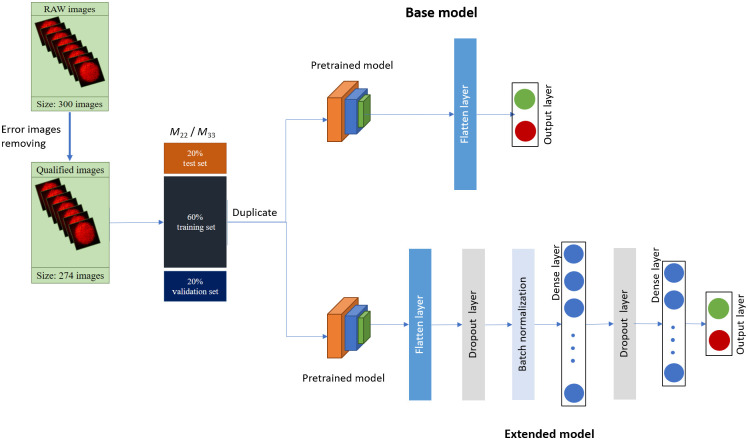
In the present study, the positive and negative HBV samples were classified using five deep learning models based on the MMIP-derived Mueller matrix elements (see Sec. 4.2). Figure 1 shows the basic architecture of the deep learning models implemented in the present study. (Note that the models were all implemented on Google Colab Pro with a Tesla P100 GPU.)
Fig. 1.
Schematic of deep learning model architecture.
For each model, 274 samples were taken as the input to the learning algorithm, with 219 samples used for training and validation purposes (i.e., 80% of the dataset) and 55 images retained for testing (i.e., 20% of the dataset). It is noted that, for the training set of MMIP images, a fivefold cross-validation technique was applied, and for solving the problem of insufficient training data, a transfer learning technique was applied in this study.39 Furthermore, the augmentation technique was applied to increase the diversification of the dataset during the training process. As shown in Fig. 1, two model variants were considered in each case: a base model and an extended model. In the base model, all of the layers were frozen, i.e., the weights pretrained on ImageNet were not modified but were used to classify the input MMIM images directly. By contrast, in the extended model, the layers were unfrozen and were thus updated during the training process in accordance with the loss function. It is noted that the dense layers were added to slowly reduce the output of the last layer of models from 1000 classes to [256, 128, 64, 32, 16] (i.e., intermediate layers) and finally to two classes. Moreover, dropout and batch normalization layers were put together with fully-connected layers (i.e., dense layers) in the model architecture to reduce overfitting. For both model variants, the binary cross entropy loss was employed, with an initial learning rate of 0.0001, the Adam optimizer, and a batch size of 32. Moreover, the classification performance was evaluated using four metrics, namely,
| (10) |
| (11) |
| (12) |
| (13) |
where TP, TN, FP, and FN denote true positive, true negative, false positive, and false negative, respectively.
Machine learning algorithms are highly susceptible to the range and distribution of the attribute values. In particular, data outliers can harm and delude the training process, resulting in prolonged training intervals and, ultimately, a poorer result. Thus, detecting and removing outliers in the input data is of crucial importance in improving the classification performance of the algorithm.40 One of the most commonly used methods for identifying outliers is the Tukey test,41 in which the outliers are defined based on the quartiles of the data, where the first quartile is the value larger than a quarter of the data, the second quartile (the median) is the value larger than half of the data, and the third quartile is the value larger than three-quarters of the data. The interquartile range is defined as , and the outliers are then defined in accordance with Tukey’s rule as
| (14) |
where IQR stands for the interquartile range ().
3. Sample Preparation and Experimental Setup
3.1. Sample Preparation
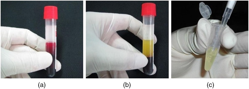
A total of 274 human serum samples were obtained from the General Central Hospital of Tien Giang Province in Vietnam between May and June 2020 [see Fig. 2(a)]. According to clinical assays, 138 of the samples were positive for HBsAg (an antigen for HBV), and 136 samples were negative. The samples were placed in serum separator tubes spray-coated with silica to assist in clotting and a polymer gel for separating the serum. The tubes were stored vertically for 20 to 30 min to form blood clots and were then centrifuged at 4000 to 5000 rpm for 10 min to separate the serum layer [see Fig. 2(b)]. The serum was extracted by a sterile plastic pipette and placed in 1.5 mL Eppendorf tubes [see Fig. 2(c)]. Finally, the tubes were stored in 100-position cryo-boxes at until required for use. The entire process was performed under the approval of the Ethics Institute of the hospital involved.
Fig. 2.
Blood sample: (a) before and (b) after centrifuging. (c) Final hepatitis serum.
Prior to the MMIP tests, two cuvettes were prepared: one for the positive samples and one for the negative samples. The cuvettes were soaked in medical alcohol at a temperature of 70°C for 15 min, rinsed with distilled water, and then left to dry. A clean micropipette was used to transfer the sample (positive or negative) from the Eppendorf tube to the cuvette. Finally, the cuvette was sealed and placed in the holder of the MMIP measurement system to evaluate its Dep properties.
3.2. Experimental Setup
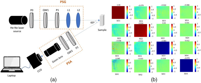
Figure 3 presents a schematic illustration of the experimental setup. As shown, the system consists mainly of a He–Ne laser as the light source (Thorlabs Inc. HRS015B, 633 nm), a polarizer (P0, Thorlabs Inc. LPVIS100-MP), a polarization state generator (PSG), a polarization state analyzer (PSA), a zoom lens (Thorlabs Inc. MVL6X12Z), a charge-coupled device (CCD) camera, and a computer. It is also noted that a coherent light source was used for the sake of simplicity and stability. The PSG creates polarized light from the unfiltered laser source, while the PSA analyzes the polarization state of the light beam scattered from the sample. The PSG comprises a quarter waveplate (QW1, Thorlabs Inc. WPQ05M-633) to generate circular polarization light, a linear polarizer (P1, Thorlabs Inc. LPVIS100-MP) to produce linear polarization light, and two condenser lenses (L1, L2, Thorlabs Inc. LSSB04-A) to focus the light onto the sample. Meanwhile, the PSA consists of a quarter waveplate (QW2, Thorlabs Inc. WPQ05M-633) and a linear polarizer (P2, Thorlabs Inc. LPVIS100-MP). In performing the measurement process, the incident angle was set to 60 deg to prevent the reflection of the incident light from the sample surface and to obtain a good polarization image.33,42 Moreover, the polarizers (P1, P2) and quarter waveplates (QW1, QW2) in the PSG and PSA were mounted on rotators (Sigma Koki Co., SGSP-60YAW-0B) to generate the 36 polarization states required to construct the Mueller matrix of each sample. In the PSG, the linear polarization states (0 deg, 45 deg, 90 deg, and 135 deg) were generated simply by rotating the polarizer (P1). The circular polarization lights (right and left) were produced by moving P1 out of the laser path with a slider and rotating the QW1 to the right- and left-hand circular polarization states. Similarly, in the PSA, the linear states of polarization were produced by rotating polarizer P2 and moving QW2 out of the laser path with a slider, whereas the circular polarization lights were generated by rotating QW2 and moving P2 out of the laser path with a slider. The principal axis angle of optical elements in the measurement system and the degree of Dep were calibrated and controlled by a commercial Stokes polarimeter (Thorlabs Inc., PAX5710). A similar calibration process was described in detail in Refs. 31 and 32. The degree of polarization of the output light is measured by commercial Stokes polarimeter and is approximately 99.99%. The calibration result of the measured Mueller matrix of a standard mirror (Thorlabs Inc., BB1-E02) with an accuracy of is shown in Fig. 3(b). It is noted that the measurement system was first developed by the Hui Ma group7,8,43 for characterizing the microstructure of biological tissue. Furthermore, the system was also employed by the present group for dengue detection.33 Thus, the feasibility of the measurement for extracting the Mueller matrix of anisotropic turbid media is confirmed. When performing the experiments, HBV samples were stored in a 1.3 mm-thickness quartz cuvette (Thorlabs Inc., CV10Q35F). It is noted that both the incident photon beam and the remission photon beam went through the isotropic cuvette sample holder. Subsequently, blood plasma is an anisotropic scattering medium but is contained in an isotropic cylinder. Therefore, the Muller matrix strongly depends on the angle at which the detector is set relative to the cuvette. The phenomenon of using an isotropic cuvette for anisotropic samples is common and well known. The simple way to eliminate the effect of the cuvette material is by dividing the measured results by the results obtained by the cuvette itself. In the current setup, the Mueller matrix is measured with 36 images. It is noted that the Mueller matrix is able to be constructed with 16 images but requires a more complicated system.44
Fig. 3.
(a) Schematic of experimental MMIM setup and (b) calibration result of measured Mueller matrix of a standard mirror.
4. Results and Discussion
4.1. Anisotropic Properties of Serum Samples
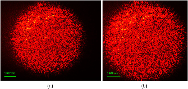
Figure 4 shows the results of HBV images before and after dropping, respectively. The original image captured from a CCD camera has the size of . For the dropping step, an average kernel was created as large as the sample (). It is noted that the size of the kernel was chosen after numerous trial and error efforts. The kernel swept across every pixel of each image. After that, the largest average intensity value was chosen, which is normally the center pixel of the image. From the center pixel, the image spread to the size of (i.e., 450 pixels in each direction). As a result, a “for” loop was used to automatically crop 274 samples (with 36 images for each sample) and save new images in PNG format.
Fig. 4.
HBV images (a) before and (b) after dropping.
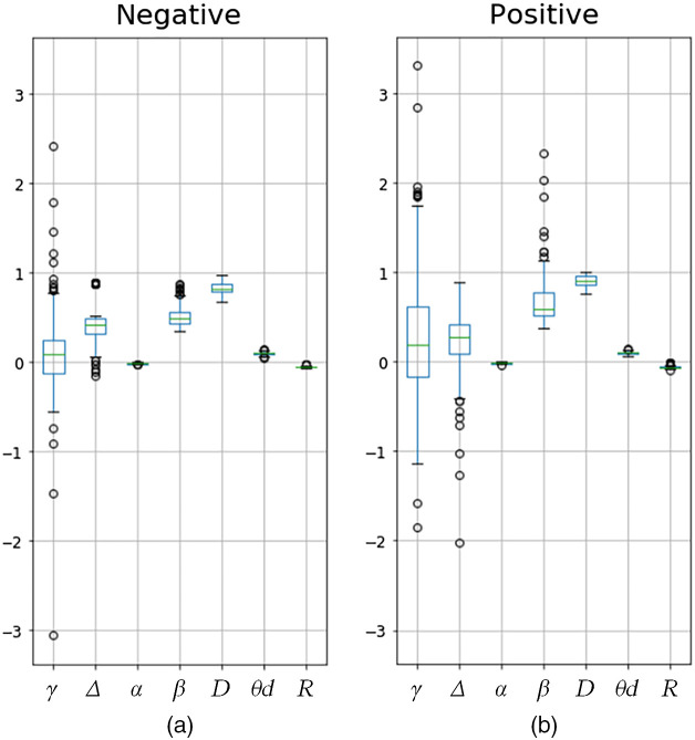
Table 1 and Fig. 5 show the values and seaborn boxplots of the anisotropic parameters of the negative and positive samples. As shown, the values of Δ provide a good discriminatory power between two samples because of the scattering properties of blood plasma. The values of Δ have a value overlap only in the range of 0.32 to 0.42, and the outliers of the positive class are much lower than those of the negative class. The value also provides a reliable indication of the sample class because of the photoelasticity properties of possible fiber structure within blood plasma. The ranges of the two classes have a minor overlap (between 0.51 and 0.55), and the outliers of the positive class have a higher value than those of the negative class. Parameters D and R can also be used to discriminate between the samples possibly containing the protein structure of antibodies (IgG or IgM) within the samples generating the dichroism properties. The values of and have overlaps between the two classes (i.e., from 0.86 to 0.876 and to , respectively). In contrast, the value range of , , and cannot be used to reliably distinguish between the two samples. is a well-known parameter used for diabetes measurement, and and are parameters for collagen and tumor structure, respectively. As shown, the outlier values of also fall within a similar range for both samples. The value ranges of and are almost the same for both classes.
Table 1.
Anisotropic parameters of negative and positive serum samples.
| Sample | Parameters | |||||||
|---|---|---|---|---|---|---|---|---|
| Negative | Mean | 0.106 | 0.440 | −0.015 | 0.509 | 0.099 | 0.836 | −0.053 |
| Std | 0.525 | 0.240 | 0.005 | 0.110 | 0.015 | 0.061 | 0.009 | |
| Min | −3.054 | −0.156 | −0.030 | 0.350 | 0.048 | 0.679 | −0.073 | |
| Max | 2.412 | 0.892 | −0.002 | 0.870 | 0.150 | 0.977 | −0.021 | |
| −0.118 | 0.319 | −0.018 | 0.428 | 0.091 | 0.790 | −0.060 | ||
| 0.243 | 0.492 | −0.011 | 0.558 | 0.109 | 0.877 | −0.048 | ||
| IQR | 0.361 | 0.173 | 0.007 | 0.130 | 0.018 | 0.086 | 0.011 | |
| Positive | Mean | 0.317 | 0.230 | −0.013 | 0.700 | 0.103 | 0.905 | −0.056 |
| Std | 0.765 | 0.431 | 0.006 | 0.300 | 0.014 | 0.060 | 0.014 | |
| Min | −1.856 | −2.016 | −0.032 | 0.372 | 0.069 | 0.763 | −0.098 | |
| Max | 3.318 | 0.892 | −0.0001 | 2.335 | 0.143 | 1.000 | −0.011 | |
| −0.161 | 0.091 | −0.017 | 0.513 | 0.093 | 0.860 | −0.065 | ||
| 0.623 | 0.423 | −0.009 | 0.776 | 0.112 | 0.958 | −0.054 | ||
| IQR | 0.784 | 0.332 | 0.008 | 0.263 | 0.019 | 0.098 | 0.011 | |
Fig. 5.
Seaborn boxplot of anisotropic parameters of serum samples: (a) negative sample and (b) positive sample.
4.2. Application of Deep Learning Models to HBV Detection
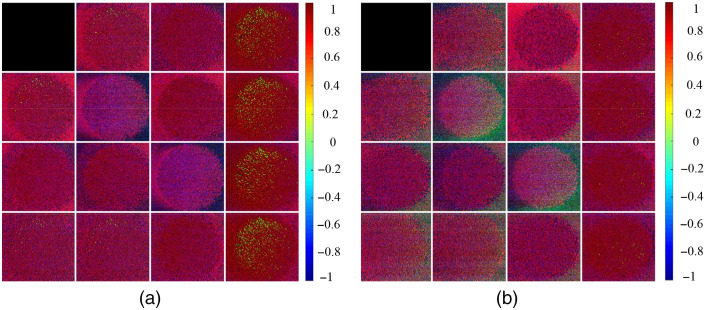
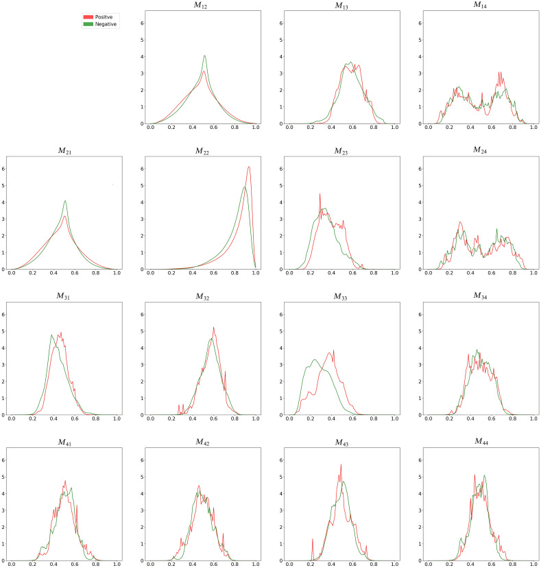
Figures 6(a) and 6(b) present illustrative Mueller matrix images of the negative and positive HbsAg samples, respectively. Figure 7 presents the corresponding kernel density estimation results. The images presented in Fig. 6 confirm that qualitative differences exist between the Mueller matrix element images of the two classes. A close inspection of Fig. 7 reveals that elements and show the greatest difference between the two classes and hence provide the most reliable elements for differentiating between them. It is noted that these results show a good quantitative agreement with those obtained from Ref. 33 and are consistent with the results reported in Ref. 45. Accordingly, two datasets consisting of and images, respectively, were prepared and supplied as inputs to five different deep learning models (Xception, VGG16, VGG19, ResNet50, and ResNet150).
Fig. 6.
Mueller matrix images in BGR color format: (a) negative sample and (b) positive sample.
Fig. 7.
Kernel density estimations of positive and negative samples.
Table 2 shows the number of positive and negative HbsAg samples used for training and testing. From 138 of the positive and 136 negative samples, 219 samples (i.e., 108 positive samples and 111 negative samples) were used for training with a fivefold cross-validation technique, and 55 samples (i.e., 30 positive samples and 25 negative samples) were used for testing.
Table 2.
Number of positive and negative HbsAg samples in training and testing datasets.
| Positive | Negative | |
|---|---|---|
| Number of training samples | 108 | 111 |
| Number of testing samples | 30 | 25 |
4.3. Base Model Results
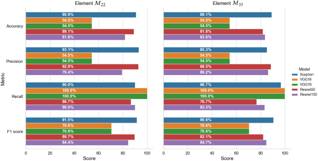
Figure 8 shows the performance metrics of the five base models when applied to the test dataset using matrix elements (a) and (b) as the input for classification purposes. Obviously, as shown in Fig. 8, the abilities of detection among the five models have significant differences. It is seen that the Xception, ResNet50, and ResNet150 models all have accuracies of . By contrast, the two VGG models have an accuracy of just 54.5%. Moreover, both models have a recall score of 100%, which indicates that they consider all of the healthy samples to be HBV samples.
Fig. 8.
Performance metrics of five base models when applied to the testing dataset.
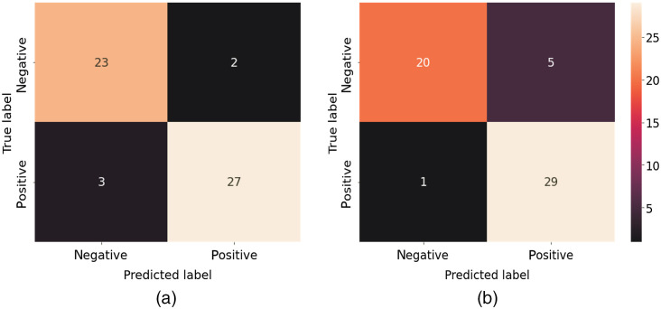
Of all models, the Xception model provides the most stable performance across the five performance metrics and achieves the highest accuracy of 90.9% and 87.3% for matrix elements and , respectively. Referring to the confusion matrixes in Fig. 9, it is seen that matrix element results in five incorrect detection cases (i.e., three FN and two FP), whereas matrix element results in six incorrect detection cases (i.e., one FN and five FP). However, matrix element results in only one positive sample being incorrectly classified as a negative (i.e., normal) sample. It is noted that, in a medical procedure of diagnosis, a highly sensitive test is when there are few FN results; in other words, few actual cases are missed.46 Therefore, usually, the prediction model with a low false negative rate will be selected.
Fig. 9.
Confusion matrixes for base the Xception model using (a) and (b) as inputs.
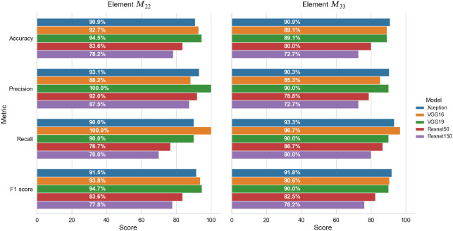
As described in Sec. 2, the base models were extended through the addition of a dropout layer, a batch normalization layer, and fully-connected layers. Keras callbacks (ModelCheckpoint, EarlyStopping, and GridsearchCV) were additionally used to optimize the training procedure. These callbacks are used to test different fully connected layer configurations with output features of [256, 128, 64, 32, 16], regularization, and kernel constraint automatically. Figure 10 shows the performance metrics of the extended models with the best output features of 32 for a fully connected layer when using matrix elements (a) and (b) as the basis for the classification process.
Fig. 10.
Performance metrics of the five extended models when applied to the testing dataset.
The Xception, VGG16, and VGG19 models all achieve an F1 score of for both matrix elements. For the case in which is taken as the basis for the classification process, the VGG19 model achieves the highest accuracy (94.5%) and F1 score (94.7%), whereas the Xception model yields the lowest accuracy (90.9%) and F1 score (91.5%). By contrast, when using element as the input, the Xception model achieves the highest F1 score (91.8%), whereas the VGG19 model achieves the lowest score (90.0%).
The ResNet models achieve a lower classification performance than the VGG and Xception models. However, the ResNet150 and ResNet50 models nevertheless achieve precision scores of 87.5% and 92%, respectively, when taking matrix element as the input to the classification process. It is noted that, in this study when using elements and as the inputs, the performance of base ResNet models achieves better results than the extended ones. This can be explained by the addition of some layers to reduce output features slowly did not guarantee an improvement in the performance of the pretrained models.
Figure 11 shows the confusion matrix of the extended VGG19 model when using matrix element as the input. As shown, all 25 negative samples are correctly classified, giving a precision score of 100% (see Fig. 10). However, 3 of the 30 positive samples are not recognized, leading to a recall score of 90%.
Fig. 11.
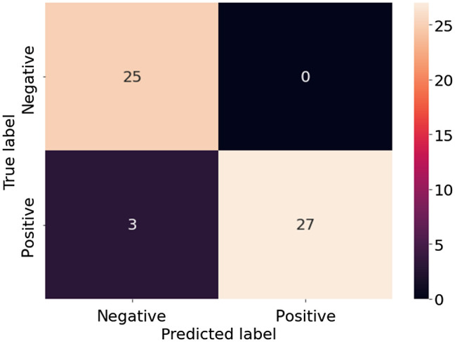
Confusion matrix of extended the VGG19 model using as input.
Figure 12 shows the confusion matrix of the extended Xception model when using matrix element as the input. It is seen that just three negative samples and two positive samples are misclassified. Thus, the precision and recall scores are equal to 90.3% and 93.3%, respectively, and the overall accuracy is 90.9%.
Fig. 12.
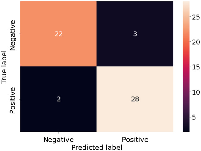
Confusion matrix of extended the Xception model using as input.
5. Conclusion
This study has proposed a combined MMIM and machine learning framework for performing the detection of HBV based on the polarization properties of blood serum samples. The results have shown that, among all of the optical anisotropic parameters of HBV serum samples, parameters , , , and provide the optimal discriminatory power between the negative and positive classes. Furthermore, five deep learning models have been considered: Xception, VGG16, VGG19, ResNet 50, and ResNet150. For each model, two variants have been implemented, namely a base model with fixed weights based on a pretrained ImageNet model and an extended model in which the weights are adjusted adaptively over the course of the training process. The results have shown that elements and of the Mueller matrix provide the maximum discriminatory power between the negative and positive samples. Moreover, among the five base models, the Xception model achieved the highest accuracy of 90.9% and 87.3% when using matrix elements and for classification purposes, respectively. By contrast, for the extended models, the optimal accuracy (94.5%) was obtained using the VGG19 model with element as the input. Overall, the results indicate that the framework proposed in this study provides a reliable and straightforward approach for detecting HBV.
Acknowledgments
This research was funded by Vietnam National University HoChiMinh City (VNU-HCM) under Grant No. NCM2020-28-01.
Biographies
Thi-Thu-Hien Pham received her BS degree in mechatronics from HCMC University of Technology, Vietnam, in 2003 and her MS degree and PhD in mechanical engineering from the Southern Taiwan University of Technology and National Cheng Kung University, Taiwan, in 2007 and 2012, respectively. She is currently an associate professor at the School of Biomedical Engineering, International University-Vietnam National University HCMC, Vietnam. Her research interests include polarized light-tissue studies, polarimetry, optical techniques in precision measurement to determine the optical properties of bio-samples or cancer detection, and AI applications.
Hoang-Phuoc Nguyen received his BS degree in biomedical engineering from International University, Vietnam National University HCMC, Vietnam, in 2021. His research interests include artificial intelligence (AI), deep learning, and machine learning techniques for cancer detection, biomedical detection, imaging polarimetry, and applications.
Ngan-Thanh Luu received her BS degree in biomedical engineering from International University, Vietnam National University HCMC, Vietnam, in 2021. Her research interests include artificial intelligence (AI), deep learning, and machine learning techniques for biosensing, skin cancer detection, cancer detection, biomedical detection, imaging polarimetry, and applications.
Ngoc Trinh Huynh received her pharmacist diploma from the University of Medicine and Pharmacy at Ho Chi Minh City, Viet Nam, in 2004 and her master’s degree in organic chemistry from the University of Caen – Basse Normandie, France, in 2005. She received her PhD in experimental and clinical pharmacology from the University of Angers, France, in 2011. She was promoted to associate professor in 2016. Currently, she is the deputy head of the Pharmacology Department, Faculty of Pharmacy, University of Medicine and Pharmacy at Ho Chi Minh City, Vietnam. Her research interests include designing certain pathological models (diabetes, cancer, skin disorders, etc.) in vitro and in vivo in animals and investigating the efficacy or the toxicity of natural products and synthetic derivatives.
Quoc-Hung Phan received his BS degree in mechanical engineering from HCM University of Technology, Viet Nam in 2004, his MS degree from the Department of Mechanical Engineering, Southern Taiwan University, Taiwan, in 2007, and his PhD from the Department of Mechanical Engineering, National Cheng Jung University, in 2016. His research interests include surface plasmon resonance, Stokes–Mueller matrix polarimetry, optical biosensing, and noninvasive glucose monitoring devices.
Thanh-Hai Le received his BS degree in mechatronic engineering from Ho Chi Minh City University of Technology, Vietnam, and his MS degree and PhD in biomechatronic engineering from Sungkyunkwan University, South Korea, in 2007 and 2011, respectively. In September 2011, he joined the HCMC University of Technology, where he is currently a lecturer in the Department of Mechatronics, Faculty of Mechanical Engineering. His current research interests are vision-guided systems; diagnostic imaging systems using MRIs, CT scans, and X-rays; industrial automation using PLC; and instructional methodology.
Biographies of the other authors are not available.
Disclosures
The authors declare no conflicts of interest.
Contributor Information
Thi-Thu-Hien Pham, Email: ptthien@hcmiu.edu.vn.
Hoang-Phuoc Nguyen, Email: hphuoc1810@gmail.com.
Thanh-Ngan Luu, Email: nganluu0903@gmail.com.
Ngoc-Bich Le, Email: lnbich@hcmiu.edu.vn.
Van-Toi Vo, Email: lnbich@hcmiu.edu.vn.
Ngoc-Trinh Huynh, Email: hntrinh@ump.edu.vn.
Quoc-Hung Phan, Email: phanquochung3@gmail.com.
Thanh-Hai Le, Email: lthai@hcmut.edu.vn.
Code, Data, and Materials Availability
No materials were used for the analysis. The code and data used to generate the results are available in the Code Ocean repository: https://codeocean.com/capsule/9493796/tree.
References
- 1.WHO, “Hepatitis B,” 2021, https://www.who.int/news-room/fact-sheets/detail/hepatitis-b (accessed 01 December 2021).
- 2.Yu Q., et al. , “A sensitive and quantitative immunochromatographic assay for HBsAg based on novel red silica nanoparticles,” Anal. Methods 11, 6103 (2019). 10.1039/C9AY02088H [DOI] [Google Scholar]
- 3.Krajden M., et al. , “Multi-measurement method comparison of three commercial hepatitis B virus DNA quantification assays,” J. Viral Hepat. 5, 415–422 (1998). 10.1046/j.1365-2893.1998.00129.x [DOI] [PubMed] [Google Scholar]
- 4.Chevrier M. C., et al. , “Detection and characterization of hepatitis B virus of anti-hepatitis B core antigen-reactive blood donors in Quebec with an in-house nucleic acid testing assay,” Transfusion 47, 1794–1802 (2007). 10.1111/j.1537-2995.2007.01394.x [DOI] [PubMed] [Google Scholar]
- 5.Khabiri A., et al. , “Compositional changes of PBL population in patients with chronic hepatitis B virus infection,” Braz. J. Infect. Dis. 5, 345–351 (2001). 10.1590/S1413-86702001000600009 [DOI] [PubMed] [Google Scholar]
- 6.Lin Y. H., et al. , “Evaluation of a new hepatitis B virus surface antigen rapid test with improved sensitivity,” J. Clin. Microbiol. 46, 3319–3324 (2008). 10.1128/JCM.00498-08 [DOI] [PMC free article] [PubMed] [Google Scholar]
- 7.Sun M., et al. , “Characterizing the microstructures of biological tissues using Mueller matrix and transformed polarization parameters,” Biomed. Opt. Express 5, 4223–4234 (2014). 10.1364/BOE.5.004223 [DOI] [PMC free article] [PubMed] [Google Scholar]
- 8.He H., et al. , “Transformation of full 4×4 Mueller matrices: a quantitative technique for biomedical diagnosis,” Proc. SPIE 9707, 97070K (2016). 10.1117/12.2210878 [DOI] [Google Scholar]
- 9.Pierangelo A., et al. , “Ex-vivo characterization of human colon cancer by Mueller polarimetric imaging,” Opt. Express 19, 1582–1593 (2011). 10.1364/OE.19.001582 [DOI] [PubMed] [Google Scholar]
- 10.Shukla P., Pradhan A., “Mueller decomposition images for cervical tissue: potential for discriminating normal and dysplastic states,” Opt. Express 17, 1600–1609 (2009). 10.1364/OE.17.001600 [DOI] [PubMed] [Google Scholar]
- 11.Du E., et al. , “Mueller matrix polarimetry for differentiating characteristic features of cancerous tissues,” J. Biomed. Opt. 19(7), 076013 (2014). 10.1117/1.JBO.19.7.076013 [DOI] [PubMed] [Google Scholar]
- 12.Wang Y., et al. , “Mueller matrix microscope: a quantitative tool to facilitate detections and fibrosis scorings of liver cirrhosis and cancer tissues,” J. Biomed. Opt. 21(27), 071112 (2016). 10.1117/1.JBO.21.7.071112 [DOI] [PubMed] [Google Scholar]
- 13.Ghosh N., et al. , “Mueller matrix decomposition for polarized light assessment of biological tissues,” J. Biophotonics 2, 145–156 (2009). 10.1002/jbio.200810040 [DOI] [PubMed] [Google Scholar]
- 14.Ossikovski R., “Differential matrix formalism for depolarizing anisotropic media,” Opt. Lett. 36, 2330–2332 (2011). 10.1364/OL.36.002330 [DOI] [PubMed] [Google Scholar]
- 15.Lee H. R., et al. , “Mueller matrix imaging for collagen scoring in mice model of pregnancy,” Sci. Rep. 11, 15621 (2021). 10.1038/s41598-021-95020-8 [DOI] [PMC free article] [PubMed] [Google Scholar]
- 16.Liu S., et al. , “Mueller matrix imaging ellipsometry for nanostructure metrology,” Opt. Express 23(13), 17316–17329 (2015). 10.1364/OE.23.017316 [DOI] [PubMed] [Google Scholar]
- 17.Liu M. J., Tian N., Yu J., “Polarization properties of mouse oocyte captured by Mueller matrix imaging,” J. Phys. Conf. Ser. 1914(1), 012040 (2021). 10.1088/1742-6596/1914/1/012040 [DOI] [Google Scholar]
- 18.Badieyan S., et al. , “Detection and discrimination of bacterial colonies with Mueller matrix imaging,” Sci. Rep. 8, 10815 (2018). 10.1038/s41598-018-29059-5 [DOI] [PMC free article] [PubMed] [Google Scholar]
- 19.Meng R., Shao C., Dong Y., “Transmission Mueller matrix imaging with spatial filtering,” Opt. Lett. 46(16), 4009–4012 (2021). 10.1364/OL.435166 [DOI] [PubMed] [Google Scholar]
- 20.Angelo J. P., Germer T., Litorja M., “Structured illumination Mueller matrix imaging,” Biomed. Opt. Express 10(6), 2861 (2019). 10.1364/BOE.10.002861 [DOI] [PMC free article] [PubMed] [Google Scholar]
- 21.Sang J. C., et al. , “Spatial frequency domain Mueller matrix imaging,” Proc. SPIE 11646, 116460E (2021). 10.1117/12.2576350 [DOI] [Google Scholar]
- 22.Krizhevsky A., Sutskever I., Hinton G. E., “ImageNet classification with deep convolutional neural networks,” Commun. ACM 60(6), 84–90 (2017). 10.1145/3065386 [DOI] [Google Scholar]
- 23.Simonyan K., Zisserman A., “Very deep convolutional networks for large-scale image recognition,” in 3rd ICLR 2015 (2015). [Google Scholar]
- 24.He K., et al. , “Deep residual learning for image recognition,” in IEEE Conf. Comput. Vision and Pattern Recognit. (CVPR), pp. 770–778 (2016). 10.1109/CVPR.2016.90 [DOI] [Google Scholar]
- 25.Francois C., “Xception: deep learning with depthwise separable convolutions,” in IEEE Conf. Comput. Vision and Pattern Recognit. (CVPR), pp. 1800–1807 (2017). 10.1109/CVPR.2017.195 [DOI] [Google Scholar]
- 26.Ma D., et al. , “MuellerNet: a hybrid 3D-2D CNN for cell classification with Mueller matrix images,” Appl. Opt. 60(22), 6682–6694 (2021). 10.1364/AO.431076 [DOI] [PubMed] [Google Scholar]
- 27.Li X., et al. , “Classification of morphologically similar algae and cyanobacteria using Mueller matrix imaging and convolutional neural networks,” Appl. Opt. 56(23), 6520–6530 (2017). 10.1364/AO.56.006520 [DOI] [PubMed] [Google Scholar]
- 28.Liu Z., et al. , “Classification of marine microalgae using low-resolution Mueller matrix images and convolutional neural network,” Appl. Opt. 59(31), 9698–9709 (2020). 10.1364/AO.405427 [DOI] [PubMed] [Google Scholar]
- 29.Ma M., Zou Y., Huang Z., “Deep learning-based automated morphology classification of electrospun ultrafine fibers from M44 element image of Muller matrix,” Optik 206, 164261 (2020). 10.1016/j.ijleo.2020.164261 [DOI] [Google Scholar]
- 30.Zhao Y. G., et al. , “Detecting giant cell tumor of bone lesions using Mueller matrix polarimetry polarization microsocpic imaging and multi-parameters fusion network,” IEEE Sens. J. 20(13), 7208–7215 (2020). 10.1109/JSEN.2020.2978021 [DOI] [Google Scholar]
- 31.Pham T. T. H., Lo Y. L., “Extraction of effective parameters of anisotropic optical materials using a decoupled analytical method,” J. Biomed. Opt. 17(2), 025006, 2012. 10.1117/1.JBO.17.2.025006 [DOI] [PubMed] [Google Scholar]
- 32.Pham T. T. H., Lo Y. L., “Extraction of effective parameters of turbid media utilizing the Mueller matrix approach: study of glucose sensing,” J. Biomed. Opt. 17(9), 0970021 (2012). 10.1117/1.JBO.17.9.097002 [DOI] [PubMed] [Google Scholar]
- 33.Le H. M., et al. , “Mueller matrix imaging polarimetry technique for dengue Dengue fever detection,” Opt. Commun. 502, 127420 (2022). 10.1016/j.optcom.2021.127420 [DOI] [Google Scholar]
- 34.Luu N. T., et al. , “Characterization of Mueller matrix elements for classifying human skin cancer utilizing random forest algorithm,” J. Biomed. Opt. 26(7), 075001 (2021). 10.1117/1.JBO.26.7.075001 [DOI] [PMC free article] [PubMed] [Google Scholar]
- 35.Luu N. T., et al. , “Classification of human skin cancer using Stokes-Mueller decomposition method and artificial intelligence models,” Optik 249, 168239 (2022). 10.1016/j.ijleo.2021.168239 [DOI] [Google Scholar]
- 36.Baba J. S., et al. , “Development and calibration of an automated Mueller matrix polarization imaging system,” J. Biomed. Opt. 7(3), 341–349 (2002). 10.1117/1.1486248 [DOI] [PubMed] [Google Scholar]
- 37.Liao C. C., Lo Y. L., “Extraction of anisotropic parameters of turbid media using hybrid model comprising differential- and decomposition-based Mueller matrices,” Opt. Express 21, 16831–16853 (2013). 10.1364/OE.21.016831 [DOI] [PubMed] [Google Scholar]
- 38.Azzam R. M. A., “Propagation of partially polarized light through anisotropic media with or without depolarization: a differential 4 × 4 matrix calculus,” J. Opt. Soc. Am. 68, 1576–1767 (1978). [Google Scholar]
- 39.Tan C., et al. , “A survey on deep transfer learning,” in Artificial Neural Networks and Machine Learning, Kůrková V., et al., Eds., Vol. 11141, Springer, Cham: (2018). [Google Scholar]
- 40.Han J., Kamber M., Data Mining: Concepts and Techniques, Morgan Kaufman Publishers; (2000). [Google Scholar]
- 41.Tukey J., Exploratory Data Analysis, Addison-Wesley Pub. Co; (1977). [Google Scholar]
- 42.Phan Q. H., Lo Y. L., “Differential Mueller matrix polarimetry technique for non-invasive measurement of glucose concentration on human fingertip,” Opt. Express 25(13), 15179–15187 (2017). 10.1364/OE.25.015179 [DOI] [PubMed] [Google Scholar]
- 43.Nan Z., et al. , “Linear polarization difference imaging and its potential applications,” Appl. Opt. 48(35), 6734–6739 (2009). 10.1364/AO.48.006734 [DOI] [PubMed] [Google Scholar]
- 44.Han C. Y., Du C. Y., Chen D. F., “Evaluation of structural and molecular variation of starch granules during the gelatinization process by using the rapid Mueller matrix imaging polarimetry system,” Opt. Express 26(12), 15851–15866 (2018). 10.1364/OE.26.015851 [DOI] [PubMed] [Google Scholar]
- 45.Dong Y., et al. , “Characterizing the effects of washing by different detergents on the wavelength scale microstructures of silk samples using Mueller matrix polarimetry,” Mol. Sci. Opt. 17(8), 1301 (2016). 10.3390/ijms17081301 [DOI] [PMC free article] [PubMed] [Google Scholar]
- 46.Maxim L. D., Niebo R., Utell M. J., “Screening tests: a review with examples,” Inhal. Toxicol. 26(13), 811–828 (2014). 10.3109/08958378.2014.955932 [DOI] [PMC free article] [PubMed] [Google Scholar]


