A personalized deep learning denoising strategy for low-count PET images

Abstract

Objective.

Deep learning denoising networks are typically trained with images that are representative of the testing data. Due to the large variability of the noise levels in PET images, it is challenging to develop a proper training set for general clinical use. Our work aims to develop a personalized denoising strategy for the low-count PET images at various noise levels.

Approach.

We first investigated the impact of the noise level in the training images on the model performance. Five 3D U-Net models were trained on five groups of images at different noise levels, and a one-size-fits-all model was trained on images covering a wider range of noise levels. We then developed a personalized weighting method by linearly blending the results from two models trained on 20%-count level images and 60%-count level images to balance the trade-off between noise reduction and spatial blurring. By adjusting the weighting factor, denoising can be conducted in a personalized and task-dependent way.

Main results.

The evaluation results of the six models showed that models trained on noisier images had better performance in denoising but introduced more spatial blurriness, and the one-size-fits-all model did not generalize well when deployed for testing images with a wide range of noise levels. The personalized denoising results showed that noisier images require higher weights on noise reduction to maximize the structural similarity (SSIM) and mean squared error (MSE). And model trained on 20%-count level images can produce the best liver lesion detectability.

Significance.

Our study demonstrated that in deep learning-based low dose PET denoising, noise levels in the training input images have a substantial impact on the model performance. The proposed personalized denoising strategy utilized two training sets to overcome the drawbacks introduced by each individual network and provided a series of denoised results for clinical reading.

Introduction

Positron Emission Tomography (PET) has been widely applied in clinics for oncology (Bar-Shalom et al., 2000; Rohren et al., 2004), cardiology (Schindler et al., 2010), and neurology (Nasrallah and Dubroff, 2013; Chen, 2001). A typical PET scan requires a standard dose of radioactive tracer injection, followed by a 60-minute waiting period allowing the tracer to be distributed and a 10 to 20 minutes scanning time during which the patients are asked to stay motionless(Beyer et al., 2000). The increasing number of PET studies each year raises concerns about the lifetime cancer risk to patients and healthcare providers due to excessive radiation exposure(Robbins, 2008). In addition, the long image acquisition time not only introduces motion artifacts on the PET image but also discomforts for the patients(Peng et al., 2021). As a result, it is desirable to reduce tracer dosage and image acquisition time. However, in this case, the detector rings will collect fewer coincidence events and result in noisier reconstructed images. It is more difficult to detect low contrast lesions in a noisier image (Yan et al., 2016).

Therefore, many conventional and deep learning (DL) methods have been proposed to improve the low count PET image quality. There are three categories of the conventional denoising algorithms: image filtering and post-processing(Chan et al., 2010; Peltonen et al., 2011; Dutta et al., 2013; Arabi and Zaidi, 2021), image translation and denoising(Lin et al., 2001; Green, 2005; Le Pogam et al., 2013), and iterative reconstruction(Somayajula et al., 2010; Riddell et al., 2001; Cheng et al., 2021). Deep-learning approach can learn both the noise distribution and the image prior information which makes it outperform many conventional methods(Wang et al., 2021a) in medical image denoising fileds, including CT(Chen et al., 2017; Gholizadeh-Ansari et al., 2020), MRI(Manjón and Coupe, 2018; Tian et al., 2022), Ultrasound(Karaoğlu et al., 2022; Khor et al., 2022), and PET(Zhou et al., 2021). Xu et al. applied a residual convolutional neural network (CNN)(Zhang et al., 2017) to denoise the ultra-low-dose (0.5% counts level) brain PET data(Xu, 2017). The results showed that aside from better noise reduction, DL-based approach better preserved fine structures and image resolution. Incorporating anatomical information from Computed Tomography (CT) and Magnetic Resonance Imaging (MRI) in the deep-learning network is an efficient way to further preserve image resolution. Xiang et al. proposed a CNN network utilizing both the low dose brain PET and the T1 MRI as the training inputs to estimate the standard dose brain PET images (Xiang et al., 2017). Cui et al. trained a U-Net (Çiçek et al., 2016) with CT or MRI image as input and the noisy PET image as label(Cui et al., 2019). The network was able to learn the intrinsic structure and denoise the low count PET image simultaneously.

However, it is hard to directly apply a lab-trained DL model in clinics. In the DL experiments, the noise levels in the testing images are usually pre-defined, so the training datasets are designed to match the testing datasets. Images previously acquired from the same imaging protocol are collected to train the network. In this case, tracer type and voxel size are matched. Even if the majority of training images are collected from different vendors and have different tracer types and voxel sizes with the testing images, transfer learning can be implemented to address this issue(Chen et al., 2020; Liu et al., 2020). However, the previous transfer learning works did not take the noise level disparity into consideration. The remaining challenge for implementing a DL-based denoising algorithm on PET data is that PET images have wide range of noise levels. Even for PET images collected from the same scanner and reconstructed using the same algorithm, the noise level can vary greatly due to different injection doses, scanning time, patient weights, tracer distribution, and so on. In a previous extremely obese patient study, when the training images had higher noise level than the obese patient images, the deep learning model introduced spatial blurriness to the testing images(Liu et al., 2021a). To the best of our knowledge, there is no supervised DL denoising for PET images generalizable for a wider noise level range.

In CT denoising, task-specific and noise reduction controllable networks have gained more interest in recent years. Shan et al proposed a modularized cascaded network to denoise low count CT images(Shan et al., 2019). Intermediate denoised CT images were obtained and evaluated by physicians in a task-dependent way. The cascaded denoising network works well on CT images with different noise levels. Wang et al. inserted a hyper-parameter in a CNN network that can control the noise reduction level in the denoised CT images(Wang et al., 2021b). In total, nine networks were trained with nine hyper-parameters which allows a personalized selection towards nine different noise-resolution trade-offs. Since PET images have a higher degree of variation in noise level than CT images, DL-based personalized denoising for low-count PET images are particularly needed. Several studies made attempts toward this goal. Kim et al. proposed a penalized function to solve the noise level disparity problem in PET iterative reconstruction((Kim et al., 2018)). A linear fitting function was applied to control the bias generated by DnCNN(Zhang et al. ,2017) which was trained on different noise level images. Another study suggested that in the training process, low dose input images with higher counts or higher noise levels had more influence on the model optimization direction, so a modified loss function taking the image noise level as a weighting factor could increase model generalizability(Liu et al., 2021b). However, there is no study investigating personalized low-count PET denoising that allows controllable noise-resolution trade-offs.

In this work, we first investigated the impact of the noise level in the training images on the model performance. Normalized standard deviation in the liver region of interest (ROI) was chosen as a surrogate of image noise. We found that the noise level in the training images had a substantial impact on the model performance. The model trained with noisier input images had better performance in denoising but led to more spatial blurring. Based on this finding, we propose a personalized denoising method. Two networks were trained using lower and higher noise level datasets as inputs, respectively. The testing result was combined by the predictions of the two networks multiplied by tunable weighting factors. In this way, the weighting factors could be easily adjusted based on the image noise level or a given task. Our personalized denoising method was evaluated on patient images and phantom images in terms of image quality and lesion detectability. We found that the optimal weighting factors are different for various tasks.

Materials and Methods

2.1. Patient dataset

195 anonymized patients’ ¹⁸F-FDG PET images acquired on a Siemens Biograph mCT at Yale-New Haven Hospital were included in this study. The patient dosage was 368.24±30.26 MBq (303.33-435.12 MBq), and patient weight was 77.27±22.91 kg (37.56-178.40 kg).

Corrections for attenuation, scatter, and randoms were included in reconstruction using the Siemens E7 tool. Images were reconstructed by the ordered-subsets expectation maximization (OSEM) method with three iterations, 21 subsets, and a voxel size of 4×4×3 mm³. A Gaussian filter with a 5-mm kernel was applied to the reconstructed image. Images were all calibrated, decay corrected, and normalized to standard uptake value (SUV) units.

The low dose PET images were simulated by uniformly decimating the list-mode data at 20%, 40%, and 60% down-sampling rates(Schaefferkoetter et al., 2019). There were five independent 20%-count replicates, two independent 40%-count replicates , and one independent 60%-count replicate rebinned from the 100%-count list-mode data. We generated two noise realizations at 20% and 40% count levels, and only one sample at the 60% count level to make sure the independence of the simulated low dose images. Among the 195 patients’ PET studies, 100 studies were randomly selected as the training datasets, 27 studies were used as validation datasets, and the remaining 68 studies were used as the testing data. Therefore, there were in total 500 images for training, 135 images for validation, and 340 images for testing.

2.2. Network architecture and training

We employed a 3D U-Net (Çiçek et al., 2016) for the denoising task, as illustrated in Figure 1. The contracting path consists of three down-sampling blocks, which are constructed by two 3×3×3 3D convolutional layers. A 2×2×2 max-pooling layer connects the down-sampling blocks. Image patch size is down-sampled from 64×64×16 to 32×32×8, and to 16×16×4. The contracting path is followed by a bottleneck, which consists of two 3×3×3 convolutional layers. The expanding path has three up-sampling blocks, and each contains an up-convolutional layer followed by two convolutional layers. The concatenating paths copy and concatenate the down-sampling layers to the up-convolutional layers.

Figure 1.

3D U-Net structure used in this study.

Due to the limitations of GPU memory, a patch-based training strategy was utilized, with the patch size set as 64×64×16 voxels. During each training iteration, 1600 patches were used and the mini-batch size was set as 64. Based on the validation set that after 240 epochs the loss remained stable, the total epoch number was set as 240. Adam optimizer was used and the learning rate was set to 0.0001 initially with the exponential decay set as 0.999 after each iteration. The training was towards minimizing the L2 loss. The total number of trainable parameters was around 7.1 million. 46G memory space was required to train the network. In the testing step, patch size was increased to 256×256×64 voxels with a 64×64×16 overlapping-tile stride. The final denoised image was combined by the predicted patches where the overlapped voxels were averaged.

Training the network using 100 images took around 72 hours and testing on 340 images took 20 hours on average. The computing source used a 48G Quadro RTX 8000 GPU card.

2.3. Analysis of noise level impact on model performance

The impact of the noise level in the training images was first investigated. To determine the noise level of each PET image, we utilized the normalized standard deviation (NSTD) within a 3-cm diameter sphere in a relatively uniform part of the liver as the surrogate of image noise(Schaefferkoetter et al., 2019). We evenly grouped the 500 training images into five groups based on their NSTD value, named as Group 1 to 5. The NSTD ranges were shown in Table 1. Group 1 contained images with the lowest noise level while Group 5 contained the noisiest images. Five sample images are shown in Figure 2. In addition, we created a set of training images named “Group All” containing 100 images randomly chosen from the 500 images, covering a large range of noise levels. In Group All, there were 20, 23, 22, 19, 16 images belong to Group 1, 2, 3, 4, 5, respectively. The NSTD distribution of the 6 groups was shown in Figure 3. Group 5 had the widest range of NSTD values and some outliers. Group All had some outliers too. The training label images were the corresponding 100% counts level images. Six networks were trained using the six group datasets, respectively. The testing dataset included 340 patient images and were also sorted into 5 groups based on the NSTD ranges similar to those of the training images. The number of testing images in each group was 67, 76, 63, 60, and 74, respectively. All six networks were evaluated on the five testing groups.

Table 1.

Ranges of liver ROI NSTD in the five groups.

Group 1	Group 2	Group 3	Group 4	Group 5
(0.060-0.113)	(0.113-0.141)	(0.141-0.166)	(0.166-0.204)	(0.204-0.540)

Figure 2.

Sample training images in each of the 5 groups.

Figure 3.

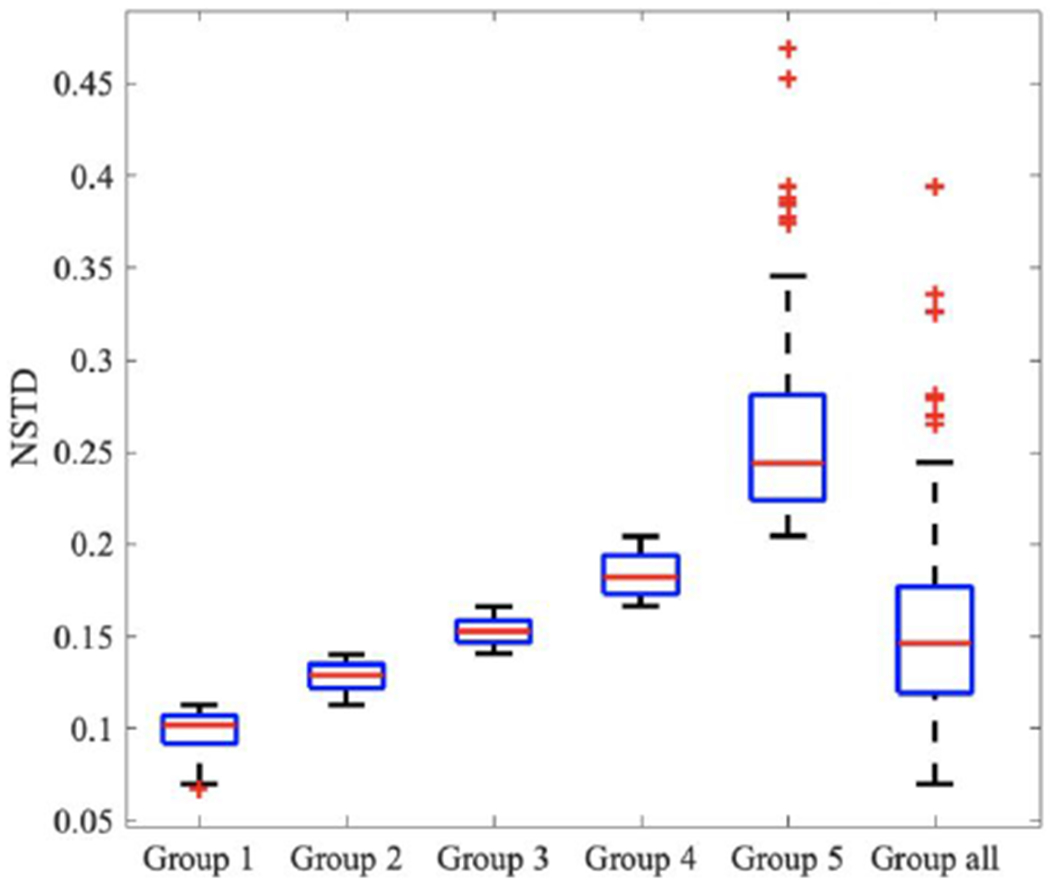
Boxplot of NSTD distribution in 6 training groups

2.4. Personalized Weighting for personalized denoising

We incorporated a blending strategy into PET denoising. Two denoised images, one has higher resolution and another has lower noise, were weighted by a tunable parameter. The overall workflow of the proposed method is shown in Figure 4. To acquire the denoised images, two 3D U-Net models were trained using 20% and 60%-count level images as inputs respectively, named as UNet 20 and UNet 60. Images denoised by these two networks were called Denoised 20 and Denoised 60. Denoised 20 were less noisy and more blurred, while Denoised 60 could better preserve the resolution but were noisier. The final denoised image was the linear blending of Denosied 20 and Denoised 60. The weighting factor was evaluated as eleven values between 0 and 1 with increments of 0.1, while in practice the weighting factor can be adjusted into any value between 0 and 1. The optimal weighting factor was determined in terms of image noise and given tasks.

Figure 4.

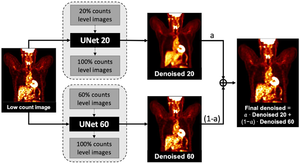
Workflow of customized denoising

We tested the customized weighting method on 340 low-dose PET images and the lung and liver lesion phantom data from the University of Pennsylvania(Surti et al., 2020). The 340 low-dose PET images were the same as the testing images used in the matched denoising study. The lung and liver lesion phantoms were the combination of the SNMMI CTN phantom (lung) with a uniform cylinder (liver) acquired on a Siemens mCT scanner. The lesion data were collected by scanning the spheres in the air. There were 16 lesions in the lung and 21 lesions in the cylinder. Both the phantom and the lesion list-mode data were combined to generate the phantom images embedded with the lesions. There were 10 replicates of the phantom datasets. For each dataset, the full scanning time was 6 min. Then each dataset was parsed into small time fractions at 0.5, 1, 1.5, 2, and 3 minutes to generate five low-count level images. There are 60 phantom images in total. Sample phantom images are shown in Figure 5.

Figure 5.

Sample slices of six noise level phantom images. The embedded lung lesions are indicated by red arrows. The embedded lung lesions are pointed by yellow arrows.

2.5. Evaluation metrics

2.5.1. Noise level

We applied NSTD as the surrogate of image noise for the human images. In the relatively uniforme liver region, we selected a 3 cm diameter sphere as the region of interest (ROI). The total number of voxels in the ROI is denoted as n. I_i, and $I_i^L$ are the SUV values in the ROI of the evaluated image and the label image. Higher the NSTD value, noisier the image

$$\text{NSTD}=\frac{\sqrt{{\sum }_i{\left(I_i-I_i^{\text{L}}\right)}^2}}{n{\sum }_i{I}_i}$$ (1)

2.5.2. Mean Squared Error (MSE)

MSE is used as a loss function and comparison method for both human and phantom images. It is defined as

$$\text{MSE}=\frac{{\sum }_i{(I_i-I_i^{\text{L}})}^2}{m},$$ (2)

where m is the total number of voxels within the human body. The background region in the PET image is excluded.

2.5.3. Peak signal-to-noise ratio (PSNR)

PSNR is defined as

$$\mathrm{PSNR}=10{\log }_{10}\left(\frac{\mathit{max}{(I^{\text{L}})}^2}{\frac{1}{\text{m}}{\sum }_{i\in \text{R}}{(I_i-I_i^{\text{L}})}^2}\right),$$ (3)

and is evaluated on the human images. Only voxels within the human body are considered.

2.5.4. Structural similarity index measure (SSIM)

SSIM is calculated by

$$\text{SSIM}=\frac{1}{N_{\text{R}}}{\sum }_{j\in \text{R}}\frac{(2{\mu }_{jx}{\mu }_{{\mathit{jx}}^L}+c_1)(2{\sigma }_{{\mathit{jx}}^L}+c_2)}{\left({\mu }_{jx}^2+{\mu }_{{\mathit{jx}}^L}^2+c_1\right)\left({\sigma }_{jx}^2+{\sigma }_{{\mathit{jx}}^L}^2+c_2\right)}\times 100\text{\%},$$ (4)

where R represents the region of interest within the human body, x and x^L represent the evaluated image and the label image, respectively. μ_jx, μ_jx^L, and ${\sigma }_{jx}^2$, ${\sigma }_{{\mathrm{jx}}^L}^2$ are the means and standard deviations in the square window on the j^th voxel of x and x^L. σ_xx^L is the covariance between x and x^L. c₁, and c₂ follow the default settings, equal to 2.55² and 7.65² respectively. It is calculated for both human and phantom images.

2.5.5. Lesion detectability

The lesion detectability was evaluated by the area under the localized receiver operating curve using the CTN phantom data. We first calculated the contrast of both background and lesions to generate the probability distribution function. Based on the two functions, the ALROC can be obtained using the below function.

$$ALROC={\int }_{-\infty }^{\infty }{f}_t(c)\ast G{(c)}^{2}dc,$$ (5)

where f(c) and g(c) are the lesion and background probability distribution functions, respectively, and G(c) is the cumulative distribution function of g(c)(Surti et al., 2020).

Results

3.1. Impact of the noise level in training images on model performance

In Figure 6, the illustrated noisy input images are down-sampled from the same 100% counts level label image. The first row 20%-count level image matches the Group 5 noise level, the second row 40%-count level image matches with Group 3, and the third row 60%-count level image is sorted into Group 1. The first colum shows the input low-count images. The middle six columns show the denoised images by different models. Model 1, Model 2, Model 3, Model 4, Model 5, and Model All U-Nets utilized training input images from Group 1, Group 2, Group 3, Group 4, Group 5, and Group All respectively. The right most column shows the same three 100% counts level label images. For the noisy input at Group 1 noise level, the MSE, PSNR, and SSIM value of input were the highest. For the noisier testing image at Group 3 noise level, the denoised MSE, PSNR, and SSIM value was the highest using Model 2. For the 20%-count images which is sorted as Group 5, Model 5 achieved the best MSE and PSNR, and Model 4 has the highest SSIM. Denoised images by Model 5 and Model All are visually less noisy than other denoised image (Pointed by the red arrows). However, Model 5 and Model All introduce more spatial blurriness. Pointed by the yellow arrows, the two lesions are merged in Model 5 and Model All images. While in the rest denoised image, the boundary between these two lesions is clear.

Figure 6.

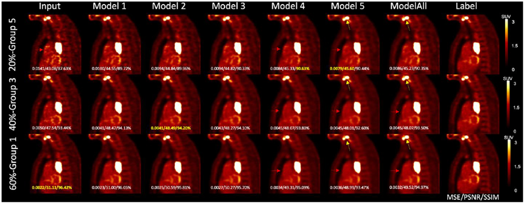
Results of matched denoising, unmatched denoising, and one-size-fits-all denoising from one sample patient. The MSE, PSNR, and SSIM values with the label image as reference are shown on each image, with the highest value shown in yellow. Yellow arrows point to the gap between two lesions. Red arrows indicate the noise reduction in the chest.

3.1.1. Noise reduction

Table 2 shows the NSTD mean and variance of the input, label, and denoised images for the five groups with the paired t-test results between the label and denoised images. The p-values higher than 0.05 are shown in the table. Compared with the input low dose images, denoised images have lower NSTD. The NSTD decreasing trend is observed for images denoised by a model trained on noisier images. For less noisy images from Group 1, the NSTDs of the denoised images by Model 1 are consistent with the label NSTDs. For noisier input images from Groups 2, 3, and 4, to get the similar denoised NSTDs with the label, the model needs to be trained on noisier images. In terms of the NSTD values. Model All has the closest performance with Model 4(p = 0.08).

Table 2.

The average NSTD value in the input, label, and denoising images

NSTD	Input	Label	Model All	Model 1	Model 2	Model 3	Model 4	Model 5
Group 1	0.097±0.012	0.072±0.011	0.058±0.008	0.073±0.010 p = 0.25	0.068±0.009	0.062±0.009	0.057±0.008	0.050±0.008
Group 2	0.127±0.008	0.087±0.017	0.078±0.009	0.097±0.008	0.092±0.008	0.084±0.009 p = 0.08	0.077±0.010	0.069±0.011
Group 3	0.152±0.007	0.093±0.016	0.093±0.008 p = 0.48	0.118±0.007	0.110±0.007	0.102±0.007	0.093±0.008 p = 0.46	0.083±0.009
Group 4	0.182±0.012	0.103±0.022	0.111±0.010	0.142±0.010	0.133±0.010	0.124±0.010	0.113±0.009	0.099±0.010 p = 0.08
Group 5	0.249±0.042	0.136±0.046	0.167±0.040	0.205±0.041	0.195±0.041	0.185±0.041	0.171±0.041	0.151±0.040

Sample images and line profiles are shown in Figure 7. The left sub-figure shows the images and line profiles of the spine in a sample Group 1 testing image. The Group 1 testing input image, label image, Model 1 denoised image, and Model 5 denoised image are shown in the upper left. The right sub-figure shows the line profile of a lesion in a Group 5 testing image, including the corresponding testing input image, label image, Model 1, and Model 5 denoised images. Model 5 led to more blurring than Model 1.

Figure 7.

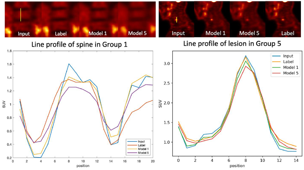
Line profile of spine in Group 1(left) and lesion in Group 3(right). Input, label, Model 1 denoised, and Model 5 denoised line profile are shown at the bottom.

3.1.3. Image Quality

MSE, PSNR, SSIM comparison results are presented in Table 3, Table 4, and Table 5, respectively. We computed the mean and standard deviation across all patients in each group. Within each group, the best model is identified by the lowest value for MSE or the highest value for PSNR and SSIM. A paired-test was performed to show the statistical significance of the best model by comparing it with the input images and other models. P-value larger than 0.05 are shown in the table. For MSE comparison, when the testing input image is from Group 1 and Group 2, Model 1 produces the lowest MSE value but doesn’t outperform the input images, which are not very noisy. For testing images from Group 3, Model 1 and Model 2 have similar superior performance. For noisier testing images from Group 4 and 5, Model 5 trained on the noisiest input images outperforms other models.

Table 3.

MSE between low dose testing images and full activity images (Mean ± SD)

Group	Input	Model All	Model1	Model2	Model3	Model4	Model5
1	0.002±0.001	0.003±0.002	0.002±0.001	0.003±0.002	0.003±0.002	0.003±0.002	0.003±0.001
2	0.004±0.002 P=0.985	0.004±0.003	0.004±0.002	0.004±0.004	0.004±0.003	0.005±0.003	0.005±0.002
3	0.006±0.003	0.005±0.002	0.005±0.002 P=0.079	0.005±0.002 P=0.054	0.005±0.002	0.005±0.002	0.005±0.002
4	0.009±0.005	0.007±0.004	0.007±0.004	0.007±0.004	0.007±0.004	0.007±0.003	0.006±0.003
5	0.018±0.013	0.012±0.008	0.014±0.010	0.013±0.009	0.012±0.009	0.012±0.008	0.010±0.007

Table 4.

PSNR between low dose testing images and full activity images (Mean ± SD)

Group	Input	Model All	Model1	Model2	Model3	Model4	Model5
1	56.09±8.49	53.55±6.67	55.18±6.98	54.53±6.52	54.33±6.73	53.38±6.89	53.35±7.30
2	53.20±7.62 P=0.482	52.40±6.03	53.25±6.47	52.90±6.09	52.82±6.21	52.27±6.16	52.34±6.34
3	51.57±6.15	52.30±5.43	52.44±5.75	52.43±5.59	52.36±5.59	52.23±5.51	52.37±5.48
4	49.40±5.53	50.58±4.87	50.42±5.12 P=0.769	50.51±4.95 P=0.241	50.49±5.00 P=0.818	50.55±4.91	50.79±4.96
5	48.75±7.28	50.17±6.32	49.77±6.76	49.90±6.50	49.91±6.54	50.20±6.35	50.63±6.30

Table 5.

SSIM between low dose testing images and full activity images (Mean ± SD)

Group	Input	Model All	Model1	Model2	Model3	Model4	Model5
1	94.57%±2.05% P=0.551	93.41%±1.29%	94.51%±1.46%	94.62%±1.47%	94.45%±1.35%	94.10%±1.24%	93.19%±1.19%
2	91.48%±3.09%	91.64%±1.69%	92.23%±2.21%	92.37%±2.17% P=0.082	92.43%±1.94%	92.29%±1.72%	91.67%±1.49%
3	87.65%±3.95%	89.35%±2.12%	89.26%±2.89%	89.44%±2.81%	89.75%±2.55%	89.92%±2.21%	89.71%±1.79%
4	85.22%±4.28%	87.56%±3.07%	87.35%±3.52%	87.35%±3.30%	87.80%±3.30%	88.12%±3.02% P=0.326	88.21%±2.71%
5	81.00%±6.35%	84.18%±5.04%	83.49%±5.65%	83.49%±5.65%	84.12%±5.43%	84.71%±5.08%	85.30%±4.50%

Similar results are observed in the PSNR comparison. Model 1 produces the highest PSNR among other models given the testing images from Group 1, 2, and 3. For testing imgaes from Group 4, all models have similar performance. For noisier testing images from Group 5, Model 5 outperforms other models with the highest PSNR.

For SSIM comparison, given the testing images from Group 1, 2, 3, and 4, Model 2, 3, 4, and 5 achieve the highest SSIM respectively. For the testing images from Group 5, Model 5 produces the highest SSIM.

3.2. Customized weighting for personalized denoising

Figure 8 shows the sagittal view of the personalized denoising results of a sample patient. Denoised images are shown in the middle five columns with five different weighting factors. Smaller weights led to images with higher resolution and noise. SSIM values are labeled on the images. Images with the highest SSIM value from the same input are framed. For 20% count level input, the highest SSIM is achieved with weight of 0.9, which means 90% from Denoised 20 and 10% from Denoised 60. For the 40% count level, the weight of 0.5 with half Denoised 20 and half Denoised 60 outperformed other weightings. For the least noisy image at 60% count level, the highest SSIM is achieved at 10% of Denoised 20 blended with 90% of Denoised 60.

Figure 8.

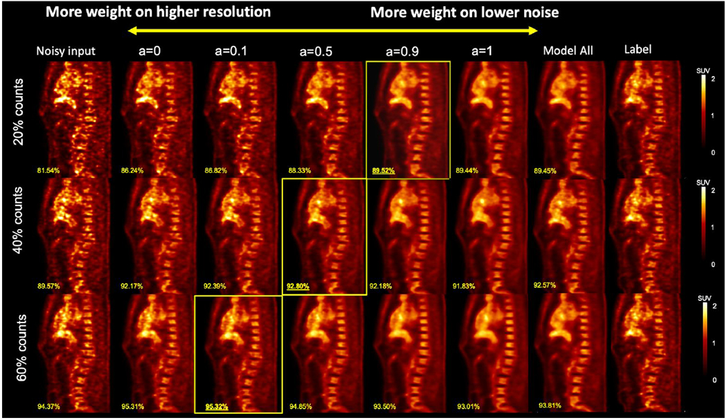
Personalized denoising results of three human images at 20%, 40%, and 60% counts levels. The weighting factor is denoted as ‘a’. The SSIM values are shown on the image in yellow. Denoised images with the highest SSIM value are framed.

Coronal views of the phantom images are shown in Figure 9. The left input images have 1.5, 2, and 3 minutes scan time, and the three same label images are shown on the right. The middle five columns show the weighted denoising results with weighting factors selected to be 0, 0.3, 0.5, 0.8, and 1. Similar performance is observed in the phantom images that noisier images require higher proportion from Denoised 20 to get the highest SSIM value.

Figure 9.

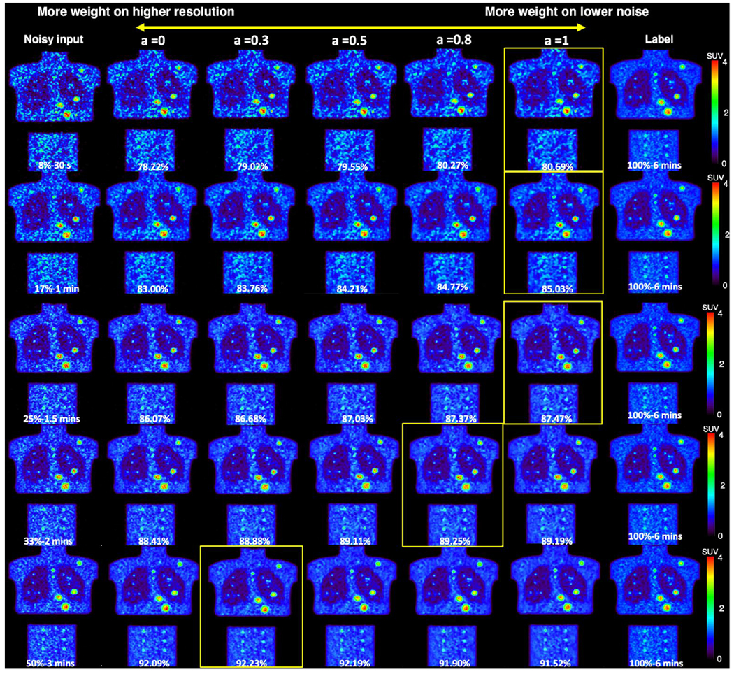
Personalized denoising results for phantom images at 8%, 17%, 25%, 33%, and 50% counts level. The weighting factor is denoted as ‘a’. The SSIM values are shown on the image in yellow. Denoised images with the highest SSIM value are framed.

3.2.1. Image quality evaluation

The SSIM and MSE using different weighting factors are shown in Figure 10. Overall, denoised images from a input with lower noise have higher SSIM and lower MSE. Both the SSIM and MSE curves show a clear trend that for noisier input, more weights on Denoised 20 are needed. The optimal weighting factors at five groups for optimizing SSIM and MSE are not always the same. For SSIM, they are 0.2, 0.4, 0.6, 0.7, 0.8, repectively for the 5 groups. For MSE, they are 0.2, 0.5, 0.6, 0.7, 0.8, repectively for the 5 groups.

Figure 10.

SSIM and MSE curves of the denoised human images. Optimal weighting factors in terms of highest SSIM and lowest MSE are marked on the curve.

The phantom SSIM and MSE curves are shown in Figure 11. When the count levels are higher than 20%, we observed the same SSIM trend with human data. However, for the MSE curve, the optimal weights are equal to 1, except for 50%, which is equal to 0.7.

Figure 11.

SSIM and MSE curves for denoised phantom images produced by customized weighting. The optimal weighting factors in terms of highest SSIM and lowest MSE are marked on the curve.

3.2.2. Lesion detectability

We plotted the lesion ALROC as shown in Figure 12. Overall, the lesions in the denoised image from higher count data are more likely to be detected. A weighting factor equal to 1 achieves the highest ALROC for a liver lesion at all noise level images, and for the lung lesion, there was no significant difference when using different weighting factors.

Figure 12.

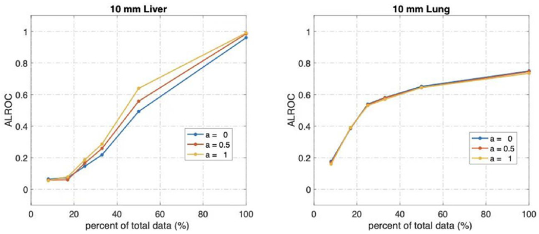
The Area under the Localized Operating Curve of liver and lung lesions.

Discussion

In this low count PET denoising study, we demonstrated the substantial impact of the noise level in the training images on the model performance and developed a personalized weighting strategy to balance the noise reduction and resolution preservation. We found that the optimal weights are affected by the image noise level and are task-driven. Given the tunable feature of the weights, it can be adjusted by physicians according to their preferences as well.

In the investigation of noise level impact, our work showed that models trained on higher noise level images have better noise reduction ability but the denoised images have a worse resolution. We also noticed that there is a noise level threshold at around NSTD smaller than 0.12 (Group 1) that performing deep learning denoising models on these images doesn’t improve the image quality. Training input images having the similar noise levels with the testing images is preferred in most cases. However, when given high noise level images, the preferred denoising model should be trained using higher noise level images as the input. If the model selection is fully dependent on better noise reduction, models trained on reasonable higher noise level images are preferred.

Model All trained on a wide range of noise level images has a similar performance with Model 4 in terms of NSTD value (p = 0.08) and Model All couldn’t outperform the matched models, which suggests that the one-size-fits-all training might not have good model generalizability. In fact, this assumption was proved in the previous study(Liu et al., 2021b). Noisier images or higher dosage have more influence in the model training procedure. A weighting matrix was applied in the loss function to diminish the impact of different dosages and noise levels. The model generalizability is improved with the modified loss function.

Based on our findings that the noise level in the training images has a substantial impact on the model performance, we propose the personalized weighting method utilizing models trained on lower noise level images and noisier images. The personalized weighting method was inspired by the widely applied adaptive statistical iterative reconstruction (ASiR™) in CT (Mangat et al., 2016; Protik et al., 2012). Compared with the filtered-back projection (FBP) reconstruction images, ASiR™ images have lower noise levels but limited spatial resolution. A linear combination of ASiR™ with FBP can achieve better image quality compared with 100% ASiR™ or FBP. In addition, the weight can be adjusted by the CT dosage and physician’s preferences(Brady and Shulkin, 2015). Practically, we envision that a similar strategy can be used for our proposed PET approach with tunable weighting factors, that can be chosen by individual users according to the PET images for a specific task. The previous deep learning studies can denoise the CT image in a personalized way, but only a fixed number of denoising degrees are available(Shan et al., 2019). Besides, some studies trained more than ten networks to achieve the goal, which consumes a fair amount of network training time(Wang et al., 2021a). Our personalized denoising only requires training two deep learning networks, and the number of alternative tunable parameters is not limited. The customized weighting method gives reasonable results on our clinical human images and lung and liver phantom images. Higher weight on the Denoised 20 is favored given noisier images, which is expected because UNet 20 has better noise reduction ability compared with UNet 60. When the testing image has a lower noise level, the weighting factor is smaller, which means the final denoised image has less contribution from Denoised 20 and more contibution from Denoised 60. By tuning the weighting factor, our customized weighting method can denoise PET images at a wide reasonable range of noise levels. In addition, the optimal weights for whole image visualization and lesion detectability are different. For liver lesions, the weighting factor equaling to 1 provides the best lesion detectability. For lung lesions, we did not observe the difference using different weighting factors, which may be due to the low activity of the lung background.(Surti et al., 2020). The personalized denoising with FDG data trained network was also applied to a sample set of low-count ⁶⁸Ga-DOTATATE images. As illustrated in Figure 13, the highest SSIM value between the denoised images with the 100%-count DOTATATE image was achieved when the weighting factor equaled 0.3 for a 30%-count image and 0 for a 50%-count image. More comprehensice evaluations are needed to demonstrate the feasibility of personzalied denoising for other tracers. Besides, the performance of personalized denoising on other tracer datasets can be improved by transfer learning(Liu et al., 2020).

Figure 13.

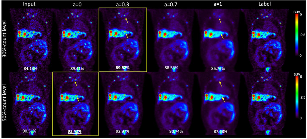
Samples of 30%-count and 50%-count DOTATATE images, and denoised images at weights 0, 0.3, 0.7, and 1. The SSIM value are shown in the bottom of each image. Weighted denoised images with the highest SSIM are framed. The yellow arrows point out lesions that were smoothed by U-Net 20.

Currently, this study focused on the simulated low dose PET image between 20% and 60% counts level, with the noise level NSTD range in 0.07 to 0.45. We have shown that when the image noise level is low (e.g. Group 1 image), DL denoising is unnessary. The performance of personalized weighting on noisier images is also not guaranteed although phantom studies show that when the image counts level is lower than 20%, the potential optimal weights should be larger than one. In this case, a model trained on noisier images is needed. In other words, the Denoised 20 should be noisier in such cases to create a wider range for the weighting strategy to tune. However, it is noted that the model trained on higher noise level images has worse spatial blurriness. Although we used Denoised 20 and Denoised 60 as examples to demonstrate our proposed weighted strategy in this study, the optimal choice of the input image noise level of the two networks in the weighted strategy depends on specific applications. In this study, the local noise level in the liver region was used as the surrogate of the whole image noise level. Since organs may have different local noise levels, further study incorporating organ segmentations will be performed to optimize the denoising for each organ. We will also examine the customized weighting on dynamic images where the noise level has large variance across frames even within the same patient.

Conclusions

In this study, we comprehensively investigated the impact of the noise level in the training images on the model performance and proposed a personalized weighting method applicable to denoised images at a wide range of noise levels. The noise level in the training images has a substantial impact on the model performance: model trained on high noise level images has stronger noise reduction ability but will introduce more spatial blurriness while model trained on low noise level images can better preserve the resolution but with inferior noise reduction. Personalized denoising is realized by individually weighting two denoised results by these two kinds of models. The optimal weighting factor is task-dependent and can be adjusted by users.

References

- Arabi H and Zaidi H 2021. Non-local mean denoising using multiple PET reconstructions Annals of nuclear medicine 35 176–86 [DOI] [PMC free article] [PubMed] [Google Scholar]
- Bar-Shalom R, Valdivia AY and Blaufox MD Seminars in nuclear medicine, 2000), vol. Series 30): Elsevier; ) pp 150–85 [DOI] [PubMed] [Google Scholar]
- Beyer T, Townsend DW, Brun T, Kinahan PE, Charron M, Roddy R, Jerin J, Young J, Byars L and Nutt R 2000. A combined PET/CT scanner for clinical oncology Journal of nuclear medicine 41 1369–79 [PubMed] [Google Scholar]
- Brady SL and Shulkin BL 2015. Ultralow dose computed tomography attenuation correction for pediatric PET CT using adaptive statistical iterative reconstruction Medical physics 42 558–66 [DOI] [PubMed] [Google Scholar]
- Chan C, Fulton R, Feng DD and Meikle S IEEE Nuclear Science Symposuim & Medical Imaging Conference,2010), vol. Series): IEEE; ) pp 3613–8 [Google Scholar]
- Chen AC 2001. New perspectives in EEG/MEG brain mapping and PET/fMRI neuroimaging of human pain International Journal of Psychophysiology 42 147–59 [DOI] [PubMed] [Google Scholar]
- Chen H, Zhang Y, Zhang W, Liao P, Li K, Zhou J and Wang G 2017. IEEE 14th International Symposium on Biomedical Imaging (ISBI 2017),2017), vol. Series): IEEE; ) pp 143–6 [Google Scholar]
- Chen KT, Schürer M, Ouyang J, Koran MEI, Davidzon G, Mormino E, Tiepolt S, Hoffmann K-T, Sabri O and Zaharchuk G 2020. Generalization of deep learning models for ultra-low-count amyloid PET/MRI using transfer learning European Journal of Nuclear Medicine and Molecular Imaging 47 2998–3007 [DOI] [PMC free article] [PubMed] [Google Scholar]
- Cheng JC, Bevington C, Rahmim A, Klyuzhin I, Matthews J, Boellaard R and Sossi V 2021. Dynamic PET image reconstruction utilizing intrinsic data-driven HYPR4D denoising kernel Medical Physics [DOI] [PubMed] [Google Scholar]
- Çiçek Ö, Abdulkadir A, Lienkamp SS, Brox T and Ronneberger O International conference on medical image computing and computer-assisted intervention, 2016), vol. Series): Springer; ) pp 424–32 [Google Scholar]
- Cui J, Gong K, Guo N, Wu C, Meng X, Kim K, Zheng K, Wu Z, Fu L, Xu B, Zhu Z, Tian J, Liu H and Li Q 2019. PET image denoising using unsupervised deep learning Eur J Nucl Med Mol Imaging 46 2780–9 [DOI] [PMC free article] [PubMed] [Google Scholar]
- Dutta J, Leahy RM and Li Q 2013. Non-local means denoising of dynamic PET images PloS one 8 e81390. [DOI] [PMC free article] [PubMed] [Google Scholar]
- Gholizadeh-Ansari M, Alirezaie J and Babyn P 2020. Deep learning for low-dose CT denoising using perceptual loss and edge detection layer Journal of digital imaging 33 504–15 [DOI] [PMC free article] [PubMed] [Google Scholar]
- Green GC 2005. Wavelet-based denoising of cardiac PET data. Carleton University; ) [Google Scholar]
- Karaoğlu O, Bilge HŞ and Uluer İ 2022. Removal of speckle noises from ultrasound images using five different deep learning networks Engineering Science and Technology, an International Journal 29 101030 [Google Scholar]
- Khor HG, Ning G, Zhang X and Liao H 2022. Ultrasound Speckle Reduction using Wavelet-based Generative Adversarial Network IEEE Journal of Biomedical and Health Informatics [DOI] [PubMed] [Google Scholar]
- Kim K, Wu D, Gong K, Dutta J, Kim JH, Son YD, Kim HK, El Fakhri G and Li Q 2018. Penalized PET reconstruction using deep learning prior and local linear fitting IEEE transactions on medical imaging 37 1478–87 [DOI] [PMC free article] [PubMed] [Google Scholar]
- Le Pogam A, Hanzouli H, Hatt M, Le Rest C C and Visvikis D 2013. Denoising of PET images by combining wavelets and curvelets for improved preservation of resolution and quantitation Medical image analysis 17 877–91 [DOI] [PubMed] [Google Scholar]
- Lin J-W, Laine AF and Bergmann SR 2001. Improving PET-based physiological quantification through methods of wavelet denoising IEEE Transactions on Biomedical Engineering 48 202–12 [DOI] [PubMed] [Google Scholar]
- Liu H, Wu J, Lu W, Onofrey JA, Liu Y-H and Liu C 2020. Noise reduction with cross-tracer and cross-protocol deep transfer learning for low-dose PET Physics in Medicine & Biology 65 185006. [DOI] [PubMed] [Google Scholar]
- Liu H, Yousefi H, Mirian N, De Lin M, Menard D, Gregory M, Aboian M, Boustani A, Chen M-K and Saperstein L 2021a. PET Image Denoising using a Deep-Learning Method for Extremely Obese Patients IEEE Transactions on Radiation and Plasma Medical Sciences [DOI] [PMC free article] [PubMed] [Google Scholar]
- Liu J, Yang Y, Wernick MN, Pretorius PH and King MA 2021. IEEE International Conference on Image Processing (ICIP),2021b), vol. Series): IEEE; ) pp 2913–7 [Google Scholar]
- Mangat J, Morgan J, Benson E, Båth M, Lewis M and Reilly A 2016. A study of the image quality of computed tomography adaptive statistical iterative reconstructed brain images using subjective and objective methods Radiation protection dosimetry 169 92–9 [DOI] [PubMed] [Google Scholar]
- Manjón JV and Coupe P International Workshop on Patch-based Techniques in Medical Imaging,2018), vol. Series): Springer; ) pp 12–9 [Google Scholar]
- Nasrallah I and Dubroff J 2013. An overview of PET neuroimaging Semin Nucl Med 43 449–61 [DOI] [PubMed] [Google Scholar]
- Peltonen S, Tuna U, Sánchez-Monge E and Ruotsalainen U 2011. IEEE Nuclear Science Symposium Conference Record,2011), vol. Series): IEEE; ) pp 3125–9 [Google Scholar]
- Peng Z, Ni M, Shan H, Lu Y, Li Y, Zhang Y, Pei X, Chen Z, Xie Q and Wang S 2021. Feasibility evaluation of PET scan-time reduction for diagnosing amyloid-β levels in Alzheimer’s disease patients using a deep-learning-based denoising algorithm Computers in Biology and Medicine 138 104919. [DOI] [PubMed] [Google Scholar]
- Protik A, Thomas K, Babyn P and Ford NL 2012. Phantom study of the impact of adaptive statistical iterative reconstruction (ASiR TM) on image quality for paediatric computed tomography [Google Scholar]
- Riddell C, Carson RE, Carrasquillo JA, Libutti SK, Danforth DN, Whatley M and Bacharach SL 2001. Noise reduction in oncology FDG PET images by iterative reconstruction: a quantitative assessment Journal of Nuclear Medicine 42 1316–23 [PubMed] [Google Scholar]
- Robbins E 2008. Radiation risks from imaging studies in children with cancer Pediatric blood & cancer 51 453–7 [DOI] [PubMed] [Google Scholar]
- Rohren EM, Turkington TG and Coleman RE 2004. Clinical applications of PET in oncology Radiology 231 305–32 [DOI] [PubMed] [Google Scholar]
- Schaefferkoetter J, Nai YH, Reilhac A, Townsend DW, Eriksson L and Conti M 2019. Low dose positron emission tomography emulation from decimated high statistics: a clinical validation study Medical physics 46 2638–45 [DOI] [PubMed] [Google Scholar]
- Schindler TH, Schelbert HR, Quercioli A and Dilsizian V 2010. Cardiac PET imaging for the detection and monitoring of coronary artery disease and microvascular health JACC Cardiovasc Imaging 3 623–40 [DOI] [PubMed] [Google Scholar]
- Shan H, Padole A, Homayounieh F, Kruger U, Khera RD, Nitiwarangkul C, Kalra MK and Wang G 2019. Competitive performance of a modularized deep neural network compared to commercial algorithms for low-dose CT image reconstruction Nature Machine Intelligence 1 269–76 [DOI] [PMC free article] [PubMed] [Google Scholar]
- Somayajula S, Panagiotou C, Rangarajan A, Li Q, Arridge SR and Leahy RM 2010. PET image reconstruction using information theoretic anatomical priors IEEE transactions on medical imaging 30 537–49 [DOI] [PMC free article] [PubMed] [Google Scholar]
- Surti S, Viswanath V, Daube-Witherspoon ME, Conti M, Casey ME and Karp JS 2020. Benefit of improved performance with state-of-the art digital PET/CT for lesion detection in oncology Journal of Nuclear Medicine 61 1684–90 [DOI] [PMC free article] [PubMed] [Google Scholar]
- Tian Q, Li Z, Fan Q, Polimeni JR, Bilgic B, Salat DH and Huang SY 2022. SDnDTI: Self-supervised deep learning-based denoising for diffusion tensor MRI NeuroImage 253 119033. [DOI] [PMC free article] [PubMed] [Google Scholar]
- Wang W, Gang GJ and Stayman JW IV Medical Imaging 2021: Physics of Medical Imaging,2021a), vol. Series 11595): International Society for Optics and Photonics; ) p 115950K [Google Scholar]
- Wang W, Gang GJ and Stayman JW 2021b. A CT Denoising Neural Network with Image Properties Parameterization and Control Proc SPIE Int Soc Opt Eng 11595. [DOI] [PMC free article] [PubMed] [Google Scholar]
- Xiang L, Qiao Y, Nie D, An L, Wang Q and Shen D 2017. Deep Auto-context Convolutional Neural Networks for Standard-Dose PET Image Estimation from Low-Dose PET/MRI Neurocomputing 267 406–16 [DOI] [PMC free article] [PubMed] [Google Scholar]
- Xu JGE; Pauly J; Zaharchuk G 2017. 200x Low-dose PET Reconstruction using Deep Learning [Google Scholar]
- Yan J, Schaefferkoetter J, Conti M and Townsend D 2016. A method to assess image quality for low-dose PET: analysis of SNR, CNR, bias and image noise Cancer Imaging 16 1–12 [DOI] [PMC free article] [PubMed] [Google Scholar]
- Zhang K, Zuo W, Chen Y, Meng D and Zhang L 2017. Beyond a gaussian denoiser: Residual learning of deep cnn for image denoising IEEE transactions on image processing 26 3142–55 [DOI] [PubMed] [Google Scholar]
- Zhou B, Tsai Y-J, Chen X, Duncan JS and Liu C 2021. MDPET: a unified motion correction and denoising adversarial network for low-dose gated PET IEEE Transactions on Medical Imaging 40 3154–64 [DOI] [PMC free article] [PubMed] [Google Scholar]