HFP‐QSMGAN: QSM from homodyne‐filtered phase images

Vincent Beliveau; Christoph Birkl; Ambra Stefani; Elke R Gizewski; Christoph Scherfler

doi:10.1002/mrm.29260

. 2022 Apr 5;88(3):1255–1262. doi: 10.1002/mrm.29260

HFP‐QSMGAN: QSM from homodyne‐filtered phase images

Vincent Beliveau ^1,^2,^✉, Christoph Birkl ^2,³, Ambra Stefani ¹, Elke R Gizewski ^2,³, Christoph Scherfler ^1,²

PMCID: PMC9323427 PMID: 35381109

Abstract

Purpose

Homodyne filtering is a standard preprocessing step in the estimation of SWI. Unfortunately, SWI is not quantitative, and QSM cannot be accurately estimated from filtered phase images. Compared with gradient‐echo sequences suitable for computing QSM, SWI is more readily available and is often the only susceptibility‐sensitive sequence acquired in the clinical setting. In this project, we aimed to quantify susceptibility from the homodyne‐filtered phase (HFP), acquired for computing susceptibility‐weighted images, using convolutional neural networks to solve the compounded problem of (1) computing the solution to the inverse dipole problem, and (2) compensating for the effects of the homodyne filtering.

Methods

Two convolutional neural networks, the U‐Net and a modified QSMGAN architecture (HFP‐QSMGAN), were trained to predict QSM maps at different TEs from HFP images. The QSM maps were quantified from a gradient‐echo sequence acquired in the same individuals using total generalized variation (TGV)‐QSM. The QSM maps estimated directly from the HFP were also included for comparison. Voxel‐wise predictions and, importantly, regional predictions of susceptibility with adjustment to a reference region, were compared.

Results

Our results indicate that the U‐Net model provides more accurate voxel‐wise predictions of susceptibility compared with HFP‐QSMGAN and HFP‐QSM. However, regional estimates of susceptibility predicted by HFP‐QSMGAN are more strongly correlated with the values from TGV–QSM compared with those of U‐Net and HFP‐QSM.

Conclusion

Accurate prediction of susceptibility can be achieved from filtered SWI phase using convolutional neural networks.

Keywords: CNN, homodyne filtering, QSM, SWI

1. INTRODUCTION

Quantitative susceptibility mapping is a recent MRI technique that has enabled the in vivo quantification of tissue magnetic susceptibility. ¹ The main strength of QSM compared with other susceptibility‐sensitive MRI techniques is that it disentangles the local magnetic field from the nonlocal contributions in gradient‐echo (GRE) phase images by solving a complex field‐to‐source ill‐posed inverse problem. ² Due to the strong paramagnetic effect of iron, QSM has been used widely to explore pathophysiology associated with iron levels within the in vivo human brain, especially in multiple sclerosis ³ and neurodegenerative diseases. ⁴

Susceptibility‐weighted imaging is a MRI technique in which the GRE phase is used to enhance the signal from GRE magnitude images. ⁵ Typically, the phase image is high‐pass‐filtered using a homodyne filter to remove unwanted phase artifacts and multiplied multiple times with the magnitude image to get the SWI. Although SWI is not a quantitative MRI technique, it is more widely adopted compared with QSM, especially in the clinical setting. As such, many clinical studies or routine examinations performed in the last decade have acquired SWI sequences. Depending on the manufacturer of the MRI system, by default, only the homodyne‐filtered phase (HFP) of the GRE sequence is stored when acquiring SWI, and, unfortunately, this phase information is not suitable for computing QSM. In older or special clinical data sets (eg, targeting a rare disease or a patient group challenging to scan with MRI), in which only the HFP images are available, the impossibility of computing accurate susceptibility values is truly a missed opportunity.

In this study we addressed the problem of estimating QSM directly from HFP images. To do this, we must solve the compounded problem of (1) computing the solution to the inverse dipole problem, and (2) compensating for the effects of the homodyne filtering. Furthermore, we investigate the possibility of predicting QSM at target TEs using a HFP image acquired at a different TE. Importantly, as measures of regional susceptibility are generally the desired endpoint of QSM analyses, our evaluation is focused toward achieving valid regional measures of susceptibility, including proper adjustment with a reference region. Furthermore, to increase reproducibility, all regions of interests are defined using a fully automatized procedure.

2. METHODS

2.1. Data set

A cohort of 13 individuals (age [years] (mean, SD) = 70.7 (7.9); sex [male/female] = 11/2) having both SWI and GRE scans available was retrospectively identified from a database at the Medical University of Innsbruck. These individuals suffered from rapid eye movement sleep behavior disorder. Regional susceptibility values in rapid eye movement sleep behavior disorder have been shown to be either in the normal range or higher, ⁶ thus providing a wider range of intensities for training. We note that this particular data set was not selected for reasons related rapid eye movement sleep behavior disorder, but represents a true scenario in which only a limited data set with both SW images and multi‐echo GRE are available, and without the possibility of acquiring more samples. The data was originally acquired as part of a study on Restless Legs Syndrome, which was approved by the local ethical board of the Medical University of Innsbruck (number AM3512 273/4.8 320/5.7 [3111a]).

2.2. Magnetic resonance imaging data acquisition

The MRI measurements were performed on a 3T whole‐body MR scanner (Magnetom Verio; Siemens). All participants underwent the same MRI protocol, including the following sequences: a coronal 3D T₁‐weighted MPRAGE sequence (TR = 1800 ms; TE = 2.19 ms; TI = 900 ms; flip angle [FA] = 9°; matrix = 416 × 160 × 512; voxel size = 0.43 × 1.2 × 0.43 mm; bandwidth = 199 Hz/pixel), a transversal 3D single‐echo GRE sequence with inline SWI computation (TR = 35 ms; TE = 20 ms; FA = 15°; matrix = 260 × 320 × 64; voxel size = 0.69 × 0.69 × 2.4 mm; bandwidth = 120 Hz/pixel; GRAPPA factor = 2), a transversal 3D multi‐echo GRE sequence (TR = 35 ms; TE = 4.92, 9.84, 14.7, 19.6, 24.6 and 29.5 ms; FA =15°; matrix = 208 × 256 × 72; voxel size = 0.9 × 0.9 × 2 mm; bandwidth = 190 Hz/pixel), and a diffusion‐weighted sequence with 20 directions and one B₀ image (TR = 6300 ms; TE = 95 ms; FA = 90°; matrix = 256 × 256 × 45; voxel size = 0.9 × 0.9 × 3.3 mm; bandwidth = 1502 Hz/pixel; GRAPPA factor = 2). Only HFP and SW images were stored for the single‐echo GRE sequence.

2.3. Predictive models

The model architecture and training procedure adopted in this work was largely derived from the QSMGAN approach proposed by Chen et al ⁷ ; we denote our model as HFP‐QSMGAN to distinguish it from the original implementation. The models were implemented in PyTorch v1.7.0. ⁸ Implementation details for the generator and discriminator of the generative adversarial network (GAN) of HFP‐QSMGAN are presented in Figure 1.

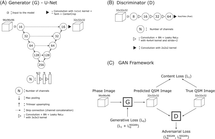
MRM-29260-FIG-0001-b — Overview of the homodyne‐filtered phase (HFP) QSM generative adversarial network (GAN) model (HFP‐QSMGAN). A, Convolutional neural network (CNN) model (U‐Net) used as image generator. B, The CNN model used as discriminator. C, Overview of the GAN framework

The generator (Figure 1A) is based on 3D implementation of the widely popular U‐Net architecture. ⁹ , ¹⁰ Importantly, we improved on the previous implementation ⁷ by replacing the transposed convolution layers by trilinear up‐sampling layers to correct for the well‐known problem of checkerboard artifacts. ¹¹ To reduce edge artifacts between patches, the model uses large input patches and crops the output of the last layer in the network, thus resulting in an increased receptive field for the final patch. We explored different input patch and cropping sizes by gradually increasing patch size and reducing cropped size, and empirically determined that an input patch of size 96 × 96 × 96 and cropping size of 32 × 32 × 32 produced minimal edge artifacts. When used on its own (ie, without adversarial training), we refer to this model as U‐Net. A content loss (ie, L1 error) was used to train the U‐Net.

For the discriminator, we adopted the same architecture as proposed by Chen et al ⁷ but adapted it to the size of the generator output (Figure 1B). To stabilize the training of the discriminator and reduce training time, a relativistic GAN ¹² was used instead of the Wasserstein GAN with the gradient penalty ¹³ proposed by Chen et al. ⁷ In relativistic GAN, the adversarial discriminator and generator loss functions are defined as

L_{D}^{RSGAN} (x_{r}, x_{f}) = - E_{(x_{r}, x_{f})} [\log (sigmoid (D (x_{r}) - D (x_{f})))]

L_{G}^{RSGAN} (x_{r}, x_{f}) = - E_{(x_{r}, x_{f})} [\log (sigmoid (D (x_{f}) - D (x_{r})))]

where x _r and x _f are real and fake (ie, generated) QSM images; D is the discriminator; and G is the generator. The full generator loss $L_{G}$ is therefore defined as

L_{G} (x_{r}, x_{f}) = {‖x_{r} - x_{f}‖}_{1} + λ \cdot L_{G}^{RSGAN} (x_{r}, x_{f})

where $λ = 0.01$ . Optimization of the discriminator and generator is performed in alternance at each minibatch update. (See Figure 1C for an overview of the GAN framework.)

2.4. Training and evaluation

Input HFP images were resampled to an isotropic resolution (0.69 mm³). Corresponding output QSM images were estimated from the phase image of the fourth, fifth, and sixth echoes of the GRE sequence (TE4 = 19.6 ms, TE5 = 24.6 ms, and TE6 = 29.5 ms) using total generalized variation (TGV)–QSM ¹⁴ ; TE after TGV‐QSM (eg, TGV‐QSM TE4) indicates that the echo of the multi‐echo GRE sequence was used by TGV‐QSM. These images were then scaled ( $\hat{x} = \tanh (10 x)$ ) and aligned with the corresponding magnitude images using Advanced Normalization Tools (rigid registration, cubic interpolation). In total, six different convolutional neural network (CNN) models were trained (both U‐Net and HFP‐QSMGAN for predicting TGV‐QSM at each of the TEs). The TE after a model name (eg, U‐Net TE4) thus denotes which TGV‐QSM maps the model was trained to predict. For comparative purposes, QSM maps were also estimated directly from the HFP using TGV‐QSM; these maps are referred to as HFP‐QSM.

The models were evaluated using a 5‐fold cross‐validation; in every fold, there were 10–11 samples available for training and 2–3 samples for testing. For each fold, the models were trained for 50 epochs using the Adam optimizer (β₁ = 0.5, β₂ = 0.999) with an initial learning rate of 1e‐5 and a batch size of 8. At each epoch, images were augmented (random affine, rotations, zooms, shears, elastic deformation, and left/right flip) and divided into nonoverlapping patches (except on the edges for complete image cover). Training each model took approximately 24 h using a NVIDIA TITAN V GPU.

2.5. Reference region

Regional QSM values were referenced to values from the posterior limb of the internal capsule (PLIC), which was previously shown to be suitable reference region for QSM. ¹⁵ To align the PLIC labels from the JHU white matter atlas ¹⁶ with the SWI (isotropic) space, the following strategy was adopted. First, fractional anisotropy maps were computed from the DWI data; preprocessing included MRtrix3's (v3.0.0) ¹⁷ denoising, unringing, and correction for eddy current and motion using FSL's eddy. ¹⁸ Then transformation from atlas space to SWI space was estimated by first aligning the corresponding atlas fractional anisotropy image to subject fractional anisotropy image (SyN registration) and B₀ image from the DWI data to the SW magnitude image (rigid registration). The PLIC label from the JHU atlas was then mapped to the SWI space (nearest‐neighbor interpolation) and eroded (1 voxel radius) to avoid any accidental overlap with the pallidum. This procedure was also used to obtain PLIC labels in the RLS data set.

2.6. Statistical analysis

All statistical analyses were performed in R v4.1 (R Foundation for Statistical Computing). ¹⁹ For evaluation purposes, only the QSM images predicted using the test data across all folds of the cross‐validation were used. The L1 errors across the susceptibility maps obtained for U‐Net and HFP‐QSMGAN at different TEs as well as from HFP‐QSM were compared using two‐sided Wilcoxon signed‐rank tests. Regional estimates of susceptibility were compared with the values obtained with TGV‐QSM using Pearson's correlation coefficients (ρ). p‐Values smaller than 0.05 were considered significant. Additionally, regional susceptibility values obtained with the CNN models were compared to those obtained with TGV‐QSM using generalized least squares (GLS) models with individual variance estimation per regions using R's nlme package (v3.1–152). ²⁰ The GLS models were fitted for the U‐Net and HFP‐QSMGAN values obtained at the three TEs, and the models were compared on the basis of the Akaike information criterion (AIC), Bayesian information criterion (BIC), and log likelihood (LL).

3. RESULTS

Examples of susceptibility maps obtained with TGV‐QSM, HFP‐QSM, U‐Net, HFP‐QSMGAN, as well as the corresponding difference maps with TGV‐QSM, are presented in Figure 2 for TE4 = 19.6 ms and Supporting Information Figures S1 and S2 for TE5 = 24.6 ms and TE6 = 29.5 ms. The HFP‐QSM map is clearly different from the TGV‐QSM map. The maps predicted by U‐Net and HFP‐QSMGAN were more similar to the TGV‐QSM map, but the U‐Net map was smoother compared with that of HFP‐QSMGAN. These observations are reflected in the difference map, where structured residuals can be seen (eg, caudate, putamen pallidum) for the HFP‐QSM map, whereas the difference maps for U‐Net and HFP‐QSMGAN appear random and unstructured.

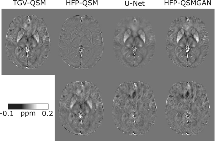
MRM-29260-FIG-0002-b — Example susceptibility maps (top) obtained for total generalized variation (TGV)–QSM (TE4 = 19.6 ms), HFP‐QSM, U‐Net and HFP‐QSMGAN, and the corresponding difference maps with the TGV‐QSM image (bottom)

Figure 3 presents the correlations between regional values for TGV‐QSM maps and predicted values obtained with the HFP‐QSMGAN TE4 model. A detailed comparison between the results of TGV‐QSM, U‐Net, HFP‐QSMGAN, and HFP‐QSM is presented in Figure 4A and Supporting Information Table S1. For only a few brain regions, HFP‐QSM values were significantly correlated with those of TGV‐QSM, whereas U‐Net and HFP‐QSMGAN were significantly correlated across almost all regions aside from the thalamus.

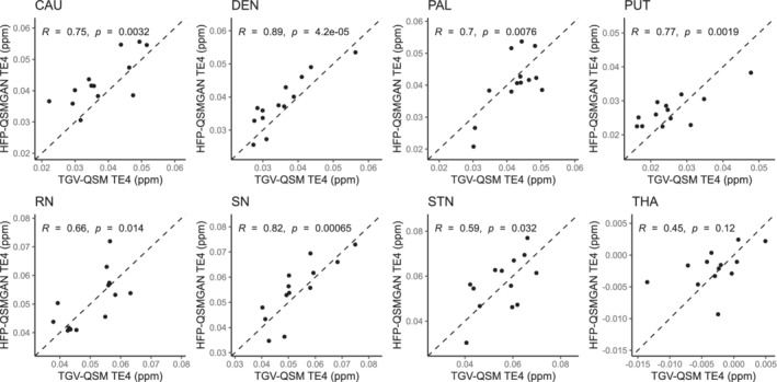
MRM-29260-FIG-0003-b — Example correlations between the estimates of regional susceptibility from TGV‐QSM and the cross‐validated values obtained from the HFP‐QSMGAN model at TE4. The dashed lines indicate identity. Abbreviations: CAU, caudate; DEN, dentate nuclei; PAL, pallidum; PUT, putamen; RN, red nuclei; SN, substantia nigra; STN, subthalamic nuclei; THA, thalamus

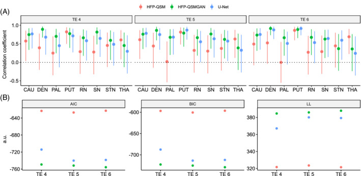
MRM-29260-FIG-0004-c — A, Pearson's correlation coefficient. B, Akaike information criterion (AIC), Bayesian information criterion (BIC), and log likelihood (LL). C, Average L1 errors for the different models. Abbreviation: a.u., arbitrary unit

GLS models were estimated, and the evaluation metrics AIC, BIC, and LL are presented in Figure 4B and Supporting Information Table S1. Lower AIC and BIC, and larger LL, correspond to better model fit. Across all echoes and metrics, the models ranked from worst to best were HFP‐QSM, U‐Net, and HFP‐QSMGAN. Performances were also always superior for the later TE (ie, results for TE5 were better than for TE4, and results for TE6 were better than for TE5).

For completeness, the average L1 errors (content loss) obtained for each susceptibility map compared with TGV‐QSM are presented in Figure 4C. Across all TEs, the U‐Net achieved significantly lower (p < 0.001) L1 errors compared with HFP‐QSMGAN and HFP‐QSM, and the L1 errors for HFP‐QSMGAN were significantly lower than that of HFP‐QSM.

4. DISCUSSION

Accurate quantification of susceptibility from SW phase images is severely impaired by homodyne filtering, which is required for SWI. In the current data set, regional QSM values quantified directly from HFP (HFP‐QSM) were generally not correlated with values quantified from unfiltered phase images acquired using multi‐echo GRE sequences (ie, TGV‐QSM). It was also apparent that QSM images generated from HFP images have a contrast that differs drastically from the QSM maps quantified from unfiltered multi‐echo GRE phase (Figure 2). In this work we have demonstrated that regional susceptibility—which is significantly correlated with a target susceptibility (ie, TGV‐QSM)—can be achieved from HFP images using CNNs. It is important to note that this is not a generic method, and that the models are specifically tuned to reconstruct images from the predefined sequence and scanner available to train the models. Domain shift (ie, the generalization of an algorithm to an input with a different distribution) is an important, unresolved issue in medical image analysis, ²¹ and it is bound to impact any task in which accuracy is heavily dependent on the distribution of the input, as is the case here. However, we have shown that even with a limited data set containing both unfiltered and HFP images, satisfying results can be achieved.

Other studies conducted in parallel to this work have also attempted to recover unfiltered phase images ²² or predict QSM ²³ from HFP images using CNNs. These studies have shown that reasonable voxel‐wise prediction was possible. In this work, we have rather concentrated on validating the regional quantification of susceptibility, including adjustment to a reference region, using a GAN model. It is well known that GAN models generate sharper images compared to CNNs without adversarial training, thus making them highly suitable for applications such as superresolution and deblurring. ²⁴ This effect is clearly apparent in Figure 2 when comparing results from the U‐Net and HFP‐QSMGAN models, with the images generated with HFP‐QSMGAN being more detailed and sharper. It is therefore interesting to note that the U‐Net achieved lower voxel‐wise L1 error compared with HFP‐QSMGAN. These results are in contrast with the initial report using QSMGAN ⁷ and may be related to the recovery of the homodyne filtering process. Nonetheless, the fit of the GLS models assessed with AIC, BIC, and LL all indicate that HFP‐QSMGAN is more accurate for the estimation of regional values with proper adjustment to a reference region, thus making it the preferred choice for predicting regional susceptibility values. Furthermore, we note that the intended goal of the models was to quantify regional susceptibility, and that L1 error does not represent an appropriate measure to assess this aim.

The question of which TE is most appropriate for assessing QSM that is most sensitive to brain iron is still not fully resolved. It was shown that the association between susceptibility and TE varies across deep gray‐matter regions and may reflect different tissue properties. ²⁵ We have demonstrated that CNNs can provide regional susceptibility estimates that are significantly correlated to the values corresponding to a different TE than the one at which the input was acquired. Beyond the current application in which QSM at a target TE is predicted from SWI phase at a different TE, this method could similarly be used to estimate QSM maps at a given TE based on the availability of GRE phase images at another TE. However, the proposed approach to generate QSM from HFP images is limited to a regional analysis of susceptibility values in gray‐matter structures. Gradient‐echo phase images, and thus QSM, are known to be sensitive to the anisotropic microstructure in white matter. ²⁶ In particular, the orientation of myelinated fibers with respect to the main magnetic field of the scanner induces a frequency shift. ²⁷ Furthermore, the fiber orientation has an impact on the TE‐dependent evaluation of the phase signal. ²⁸ Thus, for analyzing susceptibility values in white‐matter regions based on QSM retrieved from HFP images, the source and target TE should be matched as closely as possible.

A major limitation of the approach presented here is the necessity of having both the source HFP image and target GRE data acquired in the same individuals for training the models. These data may be unavailable or limited in sample size, as was the case here. Furthermore, we note that some of the structural differences observed in Figure 2 may partly be attributed to the fact that separate acquisitions were used to generate the susceptibility maps. Small sample size can be partially mitigated with proper data augmentation, which is a necessary step in almost all neuroimaging application of CNNs, but it would nonetheless hinder the generalizability of the models. Nevertheless, our results would suggest that the inference of susceptibility values from CNN models trained with limited sample size is superior for estimating susceptibility values directly from HFP images.

5. CONCLUSION

We can show that for a regional susceptibility analysis, QSM can be retrieved from HFP images acquired with standard sequences for SWI.

Supporting information

Figure S1 Example susceptibility maps (top) obtained for TGV‐QSM (TE 5 = 24.6 ms), HFP‐QSM, U‐Net and HFP‐QSMGAN, and the corresponding difference maps with the TGV‐QSM image (bottom). TE: echo time.

Figure S2 Example susceptibility maps (top) obtained for TGV‐QSM (TE 6 = 29.5 ms), HFP‐QSM, U‐Net and HFP‐QSMGAN, and the corresponding difference maps with the TGV‐QSM image (bottom). TE: echo time.

Table S1 Pearson's correlation coefficient (ρ, p‐value) between regional susceptibility estimates obtained with TGV‐QSM at different echo times as reference and HFP‐QSM, U‐Net, and HFP‐QSMGAN. GRE‐TE: echo time of the gradient echo sequence used for comparison, CAU: caudate, DEN: dendate nucleus, PAL: pallidum, PUT: putamen, RN: red nucleus, SN: substantia nigra, STN: subthalamic nucleus, THAL: thalamus.

Table S2 Evaluation metrics Akaike Information Criterion (AIC), Bayesian Information Criterion (BIC), and Log Likelihood (LL) of the different model fits.

Click here for additional data file.^{(628.8KB, docx)}

ACKNOWLEDGMENT

The authors gratefully acknowledge the support of the NVIDIA Corporation for the donation of one NVIDIA TITAN V GPU for their research.

Beliveau V, Birkl C, Stefani A, Gizewski ER, Scherfler C. HFP‐QSMGAN: QSM from homodyne‐filtered phase images. Magn Reson Med. 2022;88(3):1255‐1262. doi: 10.1002/mrm.29260

DATA AVAILABILITY STATEMENT

As data sharing was not included in the original ethics, the data used in this study cannot be made available publicly due to privacy issues. The source code for this manuscript is freely available at https://github.com/mui‐neuro/HFP‐QSMGAN.

REFERENCES

1. Deistung A, Schweser F, Reichenbach JR. Overview of quantitative susceptibility mapping. NMR Biomed. 2017;30:e3569. [DOI] [PubMed] [Google Scholar]
2. De Rochefort L, Liu T, Kressler B, et al. Quantitative susceptibility map reconstruction from MR phase data using Bayesian regularization: validation and application to brain imaging. Magn Reson Med. 2010;63:194‐206. [DOI] [PubMed] [Google Scholar]
3. Granziera C, Wuerfel J, Barkhof F, et al. Quantitative magnetic resonance imaging towards clinical application in multiple sclerosis. Brain. 2021;144:1296‐1311. [DOI] [PMC free article] [PubMed] [Google Scholar]
4. Ravanfar P, Loi SM, Syeda WT, et al. Systematic review: quantitative susceptibility mapping (QSM) of brain iron profile in neurodegenerative diseases. Front Neurosci. 2021;15:618435. [DOI] [PMC free article] [PubMed] [Google Scholar]
5. Haacke EM, Xu Y, Cheng Y‐CN, Reichenbach JR. Susceptibility weighted imaging (SWI). Magn Reson Med. 2004;52:612‐618. [DOI] [PubMed] [Google Scholar]
6. Sun J, Lai Z, Ma J, et al. Quantitative evaluation of iron content in idiopathic rapid eye movement sleep behavior disorder. Mov Disord. 2020;35:478‐485. [DOI] [PubMed] [Google Scholar]
7. Chen Y, Jakary A, Avadiappan S, Hess CP, Lupo JM. QSMGAN: improved quantitative susceptibility mapping using 3D generative adversarial networks with increased receptive field. Neuroimage. 2019;207:116389. [DOI] [PMC free article] [PubMed] [Google Scholar]
8. Paszke A, Gross S, Massa F, et al. PyTorch: an imperative style, high‐performance deep learning library. Proceedings of the 33rd International Conference on Neural Information Processing Systems. Red Hook, NY: Curran Associates Inc.; 2019;721:8026‐8037. [Google Scholar]
9. Ronneberger O, Fischer P, Brox T. U‐net: convolutional networks for biomedical image segmentation. International Conference on Medical Image Computing and Computer‐Assisted Intervention. Springer; 2015:234‐241. [Google Scholar]
10. Çiçek Ö, Abdulkadir A, Lienkamp SS, Brox T, Ronneberger O. 3D U‐net: learning dense volumetric segmentation from sparse annotation. Lecture Notes in Computer Science (Including Subseries Lecture Notes in Artificial Intelligence and Lecture Notes in Bioinformatics). Springer; 2016:424‐432. [Google Scholar]
11. Odena A, Dumoulin V, Olah C. Deconvolution and checkerboard artifacts. Distill. 2016;1:1. [Google Scholar]
12. Jolicoeur‐Martineau A. The relativistic discriminator: a key element missing from standard GAN. arXiv 2018.
13. Gulrajani I, Ahmed F, Arjovsky M, Dumoulin V, Courville A. Improved training of Wasserstein GANs. Adv Neural Inf Process Syst. 2017;2017:5768‐5778. [Google Scholar]
14. Langkammer C, Bredies K, Poser BA, et al. Fast quantitative susceptibility mapping using 3D EPI and total generalized variation. Neuroimage. 2015;111:622‐630. [DOI] [PubMed] [Google Scholar]
15. Straub S, Schneider TM, Emmerich J, et al. Suitable reference tissues for quantitative susceptibility mapping of the brain. Magn Reson Med. 2017;78:204‐214. [DOI] [PubMed] [Google Scholar]
16. Oishi K, Zilles K, Amunts K, et al. Human brain white matter atlas: identification and assignment of common anatomical structures in superficial white matter. Neuroimage. 2008;43:447‐457. [DOI] [PMC free article] [PubMed] [Google Scholar]
17. Tournier J‐D, Smith R, Raffelt D, et al. MRtrix3: a fast, flexible and open software framework for medical image processing and visualisation. Neuroimage. 2019;202:116137. [DOI] [PubMed] [Google Scholar]
18. Andersson JLR, Sotiropoulos SN. An integrated approach to correction for off‐resonance effects and subject movement in diffusion MR imaging. Neuroimage. 2016;125:1063‐1078. [DOI] [PMC free article] [PubMed] [Google Scholar]
19. R Core Team. R: A Language and Environment for Statistical Computing. Vienna, Austria: R Foundation for Statistical Computing. 2018.
20. Pinheiro J, Bates D, DebRoy S, Sarkar D. R Core Team Nlme: Linear and Nonlinear Mixed Effects Models, 2021.
21. Guan H, Liu M. Domain adaptation for medical image analysis: a survey. 2021: 1–15 [DOI] [PMC free article] [PubMed]
22. Kames C, Doucette J, Birkl C, Rauscher A. Recovering SWI‐filtered phase data using deep learning. Magn Reson Med. 2022;87:948‐959. [DOI] [PubMed] [Google Scholar]
23. Lu Z, Li J, Li Z, He H, Shi J. Reconstruction of quantitative susceptibility maps from phase of susceptibility weighted imaging with cross‐connected Ψ‐net. 2021 IEEE 18th International Symposium on Biomedical Imaging (ISBI). 2021;1:1351‐1355. [Google Scholar]
24. Ledig C, Theis L & Huszar F et al. Photo‐realistic single image super‐resolution using a generative adversarial network. In: Proceedings of the 30th IEEE Conference on Computer Vision and Visual Pattern Recognition, Honolulu, Hawaii. 2016. pp. 105–14.
25. Sood S, Urriola J, Reutens D, et al. Echo time‐dependent quantitative susceptibility mapping contains information on tissue properties. Magn Reson Med. 2017;77:1946‐1958. [DOI] [PubMed] [Google Scholar]
26. Wharton S, Bowtell R. Effects of white matter microstructure on phase and susceptibility maps. Magn Reson Med. 2015;73:1258‐1269. [DOI] [PMC free article] [PubMed] [Google Scholar]
27. Lancione M, Tosetti M, Donatelli G, Cosottini M, Costagli M. The impact of white matter fiber orientation in single‐acquisition quantitative susceptibility mapping. NMR Biomed. 2017;30:e3798. [DOI] [PubMed] [Google Scholar]
28. Wharton S, Bowtell R. Fiber orientation‐dependent white matter contrast in gradient echo MRI. Proc Natl Acad Sci. 2012;109:18559‐18564. [DOI] [PMC free article] [PubMed] [Google Scholar]

Associated Data

This section collects any data citations, data availability statements, or supplementary materials included in this article.

Supplementary Materials

Table S2 Evaluation metrics Akaike Information Criterion (AIC), Bayesian Information Criterion (BIC), and Log Likelihood (LL) of the different model fits.

Click here for additional data file.^{(628.8KB, docx)}

Data Availability Statement

[mrm29260-bib-0001] 1. Deistung A, Schweser F, Reichenbach JR. Overview of quantitative susceptibility mapping. NMR Biomed. 2017;30:e3569. [DOI] [PubMed] [Google Scholar]

[mrm29260-bib-0002] 2. De Rochefort L, Liu T, Kressler B, et al. Quantitative susceptibility map reconstruction from MR phase data using Bayesian regularization: validation and application to brain imaging. Magn Reson Med. 2010;63:194‐206. [DOI] [PubMed] [Google Scholar]

[mrm29260-bib-0003] 3. Granziera C, Wuerfel J, Barkhof F, et al. Quantitative magnetic resonance imaging towards clinical application in multiple sclerosis. Brain. 2021;144:1296‐1311. [DOI] [PMC free article] [PubMed] [Google Scholar]

[mrm29260-bib-0004] 4. Ravanfar P, Loi SM, Syeda WT, et al. Systematic review: quantitative susceptibility mapping (QSM) of brain iron profile in neurodegenerative diseases. Front Neurosci. 2021;15:618435. [DOI] [PMC free article] [PubMed] [Google Scholar]

[mrm29260-bib-0005] 5. Haacke EM, Xu Y, Cheng Y‐CN, Reichenbach JR. Susceptibility weighted imaging (SWI). Magn Reson Med. 2004;52:612‐618. [DOI] [PubMed] [Google Scholar]

[mrm29260-bib-0006] 6. Sun J, Lai Z, Ma J, et al. Quantitative evaluation of iron content in idiopathic rapid eye movement sleep behavior disorder. Mov Disord. 2020;35:478‐485. [DOI] [PubMed] [Google Scholar]

[mrm29260-bib-0007] 7. Chen Y, Jakary A, Avadiappan S, Hess CP, Lupo JM. QSMGAN: improved quantitative susceptibility mapping using 3D generative adversarial networks with increased receptive field. Neuroimage. 2019;207:116389. [DOI] [PMC free article] [PubMed] [Google Scholar]

[mrm29260-bib-0008] 8. Paszke A, Gross S, Massa F, et al. PyTorch: an imperative style, high‐performance deep learning library. Proceedings of the 33rd International Conference on Neural Information Processing Systems. Red Hook, NY: Curran Associates Inc.; 2019;721:8026‐8037. [Google Scholar]

[mrm29260-bib-0009] 9. Ronneberger O, Fischer P, Brox T. U‐net: convolutional networks for biomedical image segmentation. International Conference on Medical Image Computing and Computer‐Assisted Intervention. Springer; 2015:234‐241. [Google Scholar]

[mrm29260-bib-0010] 10. Çiçek Ö, Abdulkadir A, Lienkamp SS, Brox T, Ronneberger O. 3D U‐net: learning dense volumetric segmentation from sparse annotation. Lecture Notes in Computer Science (Including Subseries Lecture Notes in Artificial Intelligence and Lecture Notes in Bioinformatics). Springer; 2016:424‐432. [Google Scholar]

[mrm29260-bib-0011] 11. Odena A, Dumoulin V, Olah C. Deconvolution and checkerboard artifacts. Distill. 2016;1:1. [Google Scholar]

[mrm29260-bib-0012] 12. Jolicoeur‐Martineau A. The relativistic discriminator: a key element missing from standard GAN. arXiv 2018.

[mrm29260-bib-0013] 13. Gulrajani I, Ahmed F, Arjovsky M, Dumoulin V, Courville A. Improved training of Wasserstein GANs. Adv Neural Inf Process Syst. 2017;2017:5768‐5778. [Google Scholar]

[mrm29260-bib-0014] 14. Langkammer C, Bredies K, Poser BA, et al. Fast quantitative susceptibility mapping using 3D EPI and total generalized variation. Neuroimage. 2015;111:622‐630. [DOI] [PubMed] [Google Scholar]

[mrm29260-bib-0015] 15. Straub S, Schneider TM, Emmerich J, et al. Suitable reference tissues for quantitative susceptibility mapping of the brain. Magn Reson Med. 2017;78:204‐214. [DOI] [PubMed] [Google Scholar]

[mrm29260-bib-0016] 16. Oishi K, Zilles K, Amunts K, et al. Human brain white matter atlas: identification and assignment of common anatomical structures in superficial white matter. Neuroimage. 2008;43:447‐457. [DOI] [PMC free article] [PubMed] [Google Scholar]

[mrm29260-bib-0017] 17. Tournier J‐D, Smith R, Raffelt D, et al. MRtrix3: a fast, flexible and open software framework for medical image processing and visualisation. Neuroimage. 2019;202:116137. [DOI] [PubMed] [Google Scholar]

[mrm29260-bib-0018] 18. Andersson JLR, Sotiropoulos SN. An integrated approach to correction for off‐resonance effects and subject movement in diffusion MR imaging. Neuroimage. 2016;125:1063‐1078. [DOI] [PMC free article] [PubMed] [Google Scholar]

[mrm29260-bib-0019] 19. R Core Team. R: A Language and Environment for Statistical Computing. Vienna, Austria: R Foundation for Statistical Computing. 2018.

[mrm29260-bib-0020] 20. Pinheiro J, Bates D, DebRoy S, Sarkar D. R Core Team Nlme: Linear and Nonlinear Mixed Effects Models, 2021.

[mrm29260-bib-0021] 21. Guan H, Liu M. Domain adaptation for medical image analysis: a survey. 2021: 1–15 [DOI] [PMC free article] [PubMed]

[mrm29260-bib-0022] 22. Kames C, Doucette J, Birkl C, Rauscher A. Recovering SWI‐filtered phase data using deep learning. Magn Reson Med. 2022;87:948‐959. [DOI] [PubMed] [Google Scholar]

[mrm29260-bib-0023] 23. Lu Z, Li J, Li Z, He H, Shi J. Reconstruction of quantitative susceptibility maps from phase of susceptibility weighted imaging with cross‐connected Ψ‐net. 2021 IEEE 18th International Symposium on Biomedical Imaging (ISBI). 2021;1:1351‐1355. [Google Scholar]

[mrm29260-bib-0024] 24. Ledig C, Theis L & Huszar F et al. Photo‐realistic single image super‐resolution using a generative adversarial network. In: Proceedings of the 30th IEEE Conference on Computer Vision and Visual Pattern Recognition, Honolulu, Hawaii. 2016. pp. 105–14.

[mrm29260-bib-0025] 25. Sood S, Urriola J, Reutens D, et al. Echo time‐dependent quantitative susceptibility mapping contains information on tissue properties. Magn Reson Med. 2017;77:1946‐1958. [DOI] [PubMed] [Google Scholar]

[mrm29260-bib-0026] 26. Wharton S, Bowtell R. Effects of white matter microstructure on phase and susceptibility maps. Magn Reson Med. 2015;73:1258‐1269. [DOI] [PMC free article] [PubMed] [Google Scholar]

[mrm29260-bib-0027] 27. Lancione M, Tosetti M, Donatelli G, Cosottini M, Costagli M. The impact of white matter fiber orientation in single‐acquisition quantitative susceptibility mapping. NMR Biomed. 2017;30:e3798. [DOI] [PubMed] [Google Scholar]

[mrm29260-bib-0028] 28. Wharton S, Bowtell R. Fiber orientation‐dependent white matter contrast in gradient echo MRI. Proc Natl Acad Sci. 2012;109:18559‐18564. [DOI] [PMC free article] [PubMed] [Google Scholar]

PERMALINK

HFP‐QSMGAN: QSM from homodyne‐filtered phase images

Vincent Beliveau

Christoph Birkl

Ambra Stefani

Elke R Gizewski

Christoph Scherfler