Evolution and development of inflorescences and floral symmetry in Solanaceae

Abstract

Premise

The inflorescences of Solanaceae are unique and complex, which has led to long‐standing disputes over floral symmetry mainly due to different interpretations of the cyme‐like inflorescence structure. The main disagreements have been over how the phyllomes associated with the flower were arranged relative to the inflorescence axis especially during early flower initiation.

Methods

Here we investigated the evolution of inflorescences in Solanaceae by analyzing inflorescence structure in the context of phylogeny using ancestral state reconstruction (ASR) to determine the evolutionary transitions between loosely arranged and tightly clustered inflorescences and between monochasial‐like and dichasial‐like cymes. We also reconstructed two‐ and three‐dimensional models for 12 solanaceous species that represent both inflorescence and phylogenetic diversity in the family.

Results

Our results indicate that the most recent common ancestor of Solanaceae had a loosely arranged and monochasial‐like cyme, while tightly clustered inflorescences and dichasial‐like cymes were derived. Compared to the known process of scorpioid cyme evolution, Solanaceae achieved their scorpioid cyme‐like inflorescences through a previously undescribed way. Along the pedicel, the two flower‐preceding prophylls are not in the typical transverse position of dicotyledonous plants; they frequently have axillary buds, and the main inflorescence axis continues in a sympodial fashion. As a result, the plane of symmetry of the flower is 36° from the median, and the inflorescence axis and the two flower‐preceding prophylls are symmetrically located along that plane.

Conclusions

A better understanding of the morphological evolution of solanaceous inflorescence structure helped clarify the floral symmetry of Solanaceae.

Flowering plants often bear flowers in clusters, also known as inflorescences (Bentham, 1892; reviewed by Parkin, 1914). Inflorescence diversity is the result of different branching patterns. The two extreme forms of branching patterns are racemose and cymose (Roeper, 1826; Hofmeister, 1868; Eichler, 1875–1878; Endress, 2010; also see monotelic and polytelic classification system in Troll, 1969; Weberling, 1988, 1989). In the racemose pattern, a single apical meristem gives rise to the main axis of the inflorescence, and the flowers are all axillary; this process is also called monopodial growth (Hofmeister, 1868; Eichler, 1875–1878; Endress, 2010). In contrast, the apical meristem of the cymose pattern is terminated by developing a flower, an axillary meristem grows out and is terminated by a flower, and the process repeats itself (Hofmeister, 1868; Eichler, 1875–1878; Endress, 2010). This branching pattern with the repeated conversion of the apical meristem to a flower and the shift of the growth to the axillary meristem is also called sympodial growth (Hofmeister, 1868; Eichler, 1875–1878; Endress, 2010). Cymose branching patterns were thought to be derived from racemose branching patterns during angiosperm evolution (Kusnetzova, 1988; Endress and Doyle, 2009; reviewed by Endress, 2010). Inflorescence topology and flowering sequence may reflect adaptation to ecological factors (Prusinkiewicz et al., 2007; reviewed by Kirchoff and Claßen‐Bockhoff, 2013). For example, inflorescence structure determines the presentation of flowers; it can affect pollen transfer efficiency and eventually influence the plant's reproductive success (reviewed by Endress, 2010; Kirchoff and Claßen‐Bockhoff, 2013). Moreover, particular inflorescence types have repeatedly evolved in quite separate lineages; thus, inflorescence morphologies are highly homoplastic (Prenner et al., 2009 and references therein).

The Solanaceae family was thought to possess thyrsoids with predominantly scorpioid cymes (also called a cincinnus) (Danert, 1958; Endress, 2010). This cymose branching pattern also evolved independently in other groups such as Boraginaceae, Caryophyllaceae, and Gentianaceae (Child, 1979; Weberling, 1989; Barboza et al., 2016) and was proposed to have evolved from a compound dichasium with a bilateral branching pattern (Figure 1; Parkin, 1914; Stebbins, 1973). Dichasial cymes are relatively rare in Solanaceae but can be found in e.g., Datura, Physalis, Margaranthus, and Capsicum (reviewed by Child, 1979). In a conventional compound dichasial cyme (Figure 1A), the successive branches are at right angles, growing from axils of the prophylls; however, if the branch on one side does not develop, but aborts, abortion on alternate sides results in a scorpioid or zig‐zagging cyme (Figure 1B and C). The structure of the scorpioid‐like cyme in Solanaceae, however, is more complex than this standard model (Eichler, 1875−1878; Danert, 1958; reviewed by Child, 1979). In Solanaceae, there are often two phyllomes, not one, as the model above might suggest, associated with each flower growing along the inflorescence, and vegetative shoots grow out from the axils of these phyllomes in some species (Figure 1D; Goebel, 1931; Child, 1979; Weberling, 1989). This pattern suggests that a different process underlies the development of scorpioid, cyme‐like inflorescences in Solanaceae.

Figure 1.

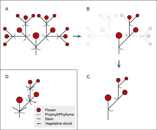
The conventional evolution of the scorpioid cyme (A–C); branching on alternate sides of a compound dichasium is suppressed resulting in a scorpioid cyme. Scorpioid cyme‐like inflorescences of Solanaceae (D) differ; here many scorpioid cyme‐like inflorescences have two flower‐preceding prophylls associated with each flower that may develop axillary vegetative shoots (D). A–C are modified from Parkin (1914) and Stebbins (1973, 1974).

Indeed, these scorpioid cyme‐like inflorescences vary extensively in Solanaceae. Thus, the phyllomes and the axillary shoots that grow along the inflorescence axis vary in number and position. Solanaceae such as Browallia speciosa Hook. and Calibrachoa elegans (Miers) Stehmann & Semir bear phyllomes along the inflorescence in between the flowers (Goebel, 1931; Child, 1979; Weberling, 1989). Other species like Juanulloa mexicana (Schltdl.) Miers have highly reduced phyllomes, while in Solanum lycopersicum L. the phyllomes are completely aborted, the inflorescences consisting of tightly clustered flowers alone (Hunziker, 2001; Welty et al., 2007). Studies on the genetic basis of inflorescence development in Solanaceae, which have focused on the dynamic interplay between determinate and indeterminate growth of the floral and inflorescence meristems, have started to improve our understanding of the inflorescence diversity in this family (Prusinkiewicz et al., 2007; Park et al., 2012, 2014; Lemmon et al., 2016; also reviewed by Ma et al., 2017; Wang et al., 2018). Since the development of phyllomes along the inflorescence is a crucial variable in inflorescence diversity in Solanaceae, the evolutionary shifts between inflorescences with loosely arranged flowers and those with tightly clustered flowers, which involve the modification of the phyllomes, needs further exploration.

There are also long‐standing disputes about the early floral orientation in Solanaceae, mainly due to the different interpretations of the complex inflorescence structures. Most species of Solanaceae have actinomorphic flowers, but those of many early‐branching lineages are zygomorphic (Knapp, 2010; Zhang et al., 2017). The two fused carpels were described as always oblique, being 36° off the median plane as defined by a line that passes through the inflorescence axis and an oppositely‐positioned flower‐subtending phyllome—and this median plane is independent of the floral symmetry of the species (Figure 2A; Wydler, 1866; Eichler, 1875–1878). When zygomorphy is established in floral whorls other than the gynoecium, it develops along the same oblique plane. The 36° oblique plane of floral zygomorphy was first noted by Wydler (1866) based on his study of the zygomorphic‐flowered Schizanthus grahamii Gillies. Eichler (1875–1878) later examined multiple solanaceous genera and found the 36° tilt in all genera except for Nicandra Adans. Robyns (1931) also agreed that Solanaceae had a 36° oblique plane of floral symmetry, but he described only the position of the gynoecium and did not mention the arrangement of the phyllomes associated with the flower (Figure 2B). The single dorsal petal evident in zygomorphic flowers in Solanaceae was the result of a 36° resupination before anthesis. However, the 36° oblique plane model was challenged by researchers such as Grau and Grönbach (1984), who thought floral zygomorphy was the result of a 180° resupination before anthesis based on their study of the genus Schizanthus (Figure 2C). Several other researchers thought that Solanaceae have a rare medial dorsal petal orientation and that the plane of floral symmetry formed along this median plane (Figure 2D) (Ampornpan and Armstrong, 1988, 1989, 1990, 1991, 2002; Ampornpan, 1992). Such disputes are primarily rooted in disagreements over the positions of the floral organs relative to the inflorescence axis and the associated phyllomes and when the different organ initiation patterns and planes of floral symmetry might imply distinct developmental processes (Bukhari et al., 2017). The study of inflorescence morphology with a focus on the relative positions of structures surrounding the flower is, therefore, a critical step to our understanding of floral development in Solanaceae.

Figure 2.

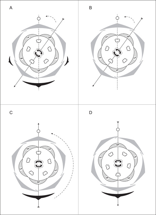
Summary of major disputes over the development of floral zygomorphy in Solanaceae. Wydler (1866) and Eichler (1875–1878) described floral zygomorphy as being established along a 36° oblique plane (A). Robyns (1931) agreed with the 36° oblique plane of floral symmetry, but he omitted the prophylls in his floral diagram (B). Two models do not recognize the 36° oblique plane; Grau and Grönbach (1984) suggested a 180° resupination in Schizanthus hookeri Gillies ex Graham (C); Ampornpan and Armstrong (2002) proposed that the flower zygomorphy is vertical along the median plane from a very early stage (D: note that the basic orientation of the floral organs differs compared to A–C). Black arcs indicate phyllomes associated with a flower; dotted lines indicate the flower's median plane (defined by the positions of the axis and the flower‐subtending bract or the center of the flower); straight arrows indicate the plane of floral symmetry, the arrowhead indicating the median abaxial position at anthesis; the dotted arc with arrowhead shows the rotation of the plane of floral symmetry before anthesis. DP, dorsal petal; LP, lateral petal; VP, ventral petal.

In this study, we investigated the evolutionary transitions of inflorescence structures in Solanaceae by carrying out ancestral state reconstructions (ASRs) on a species‐level phylogeny. We were particularly interested in the evolution of inflorescence structure when comparing loosely arranged and tightly clustered inflorescences and monochasial‐ and dichasial‐like sympodial‐branching patterns. We also reconstructed 2‐dimensional (2D‐) and 3D‐models to compare the inflorescence structures of 12 solanaceous species from 10 genera representing morphologically and phylogenetically diverse lineages by studying living samples. On the basis of the 2D and 3D modeling, we describe the basic unit of solanaceous inflorescences and propose a model to explain how the scorpioid, cyme‐like inflorescences of Solanaceae result from modifications of this basic structure by a process distinct from the existing model of the evolution of scorpioid cymes. Most importantly, we discuss how misunderstandings of inflorescence structure and its evolution have led to the disputes over floral development. Our results suggest that the scorpioid cyme‐like inflorescences in Solanaceae result from an undescribed developmental process and clarify the development of floral zygomorphy in Solanaceae.

MATERIALS AND METHODS

Term usages

Phyllome is a collective term for all types of leaves of a plant (Stevens, 2001 onward). The prophyll is the first phyllome (usually in monocots) or two phyllomes (usually in dicots) formed on an axillary shoot; each may subtend a shoot or a flower (Blaser, 1944; Stevens, 2001). A prophyll is often called a bracteole or flower‐preceding prophyll (FPP) when borne along a pedicel (Stevens, 2001 onward; Prenner et al., 2009). A pherophyll is a phyllome subtending an axillary shoot or flower (Stevens, 2001 onward; Endress, 2010), and is often called a bract or flower‐subtending bract (FSB) when subtending a flower and growing along with the previous branch order (Stevens, 2001 onward; Prenner et al., 2009). So, in a cymose pattern, FPPs become FSBs of the next‐order flowers. The FSB always opposes the axis it grows on, and FPPs in dicotyledonous plants occur in pairs inserted in a more or less transverse fashion (opposite or alternate) (Weberling, 1989). In our study, we use FPPs to indicate the phyllomes growing along the inflorescence axis.

We use dorsal and ventral to define the upper and lower parts of a zygomorphic flower as displayed to its pollinators at the stage of anthesis (Bukhari et al., 2017).

ASRs of the inflorescence structures

We carried out the ASR analyses for inflorescence structures on a species‐level phylogeny that included 1054 species representing 93 of the 98 accepted genera of Solanaceae and also on a genus‐level phylogeny pruned from the species‐level tree (Särkinen et al., 2013; Dupin et al., 2017; Zhang et al., 2017). Ten species that represent the other families of Solanales sensu APG IV (i.e., Convolvulaceae, Montiniaceae, Sphenocleaceae and Hydroleaceae; APG IV et al., 2016) were included as outgroups.

First, we examined character evolution by comparing inflorescences with FPPs in between flowers and inflorescences with flower clusters that lack FPPs. Here, “loosely arranged inflorescences” have conspicuous FPP(s) associated with each flower and long internodes separating these flowers; this type of inflorescence usually has vegetative phyllomes growing between flowers (Hunziker, 2001; Barboza et al., 2016). In “tightly clustered inflorescences,” the FPP(s) and internodes are usually highly reduced, and the flowers are clustered together (Hunziker, 2001; Barboza et al., 2016). The character state of each species was determined based on descriptions in previous taxonomic studies or botanical drawings (for a complete list of references, see Appendix S1).

We then examined character transitions between the two sympodial branching patterns (i.e., dichasial cymose versus monochasial cymose). We first determined whether an inflorescence has “monochasial branching”, the branching being one‐sided and resulting in a zigzag pattern (e.g., Figure 1B–D), or “dichasial branching,” the branching being on both sides and resulting in a forking pattern (Figure 1A). For genera having species with both dichasial and monochasial inflorescences, we coded them as being dichasial only if dichasia are common in those genera. The character states were based on morphological descriptions, illustrations, and photographs from previous taxonomic studies (e.g., Hunziker, 2001; Barboza et al., 2016; see Appendix S1). The inflorescence structures of the outgroups are coded using the same standards (references in Appendix S1). If the branching pattern of an outgroup was neither monochasial nor dichasial, we coded it as “other”.

The ASR analyses for the first test were performed using both maximum likelihood (ML) and Bayesian approaches on the species‐level phylogeny. For the ML inference, the analyses were carried out in Mesquite version 3.10 (Maddison and Maddison, 2017). We determined the best‐fitting model between the Mk1 (one‐parameter model) and AsymmMk (two‐parameter model) by evaluating the likelihood ratios. The Mk1 model presumes that the rates of changes between the two character states, e.g., from “loosely arranged inflorescence” to “tightly clustered inflorescence,” and vice versa, are equal, while the AsymmMk model allows the rates of change to be different. For the Bayesian inference, the stochastic character mapping (SCM) implemented using the make.simmap function in phytools version 0.5−38 (Bollback, 2006; Revell, 2012). The best‐fitting model for our data set was first determined using three models, i.e., equal rates (ER), symmetric rates (SYM), or all rates different (ARD), using the fitMk function in phytools version 0.5−38 (Revell, 2012). The rates of state transitions were then estimated based on the best‐fitting model. The posterior distribution of the transition rates was then determined using a Markov chain Monte Carlo (MCMC) simulation that ran for 10,000 generations, sampling every 100 generations. One hundred simulations were carried out for stochastic character evolution at each node (Nielsen, 2002; Huelsenbeck et al., 2003). We then summarized the ASR results on a genus‐level phylogeny that had been pruned from the species‐level phylogeny following Zhang et al. (2017). Only character states at nodes with 60% or higher support values were reported for this phylogeny.

The ASR analyses for the second test concerning the transitions between the dichasial and monochasial sympodial branching patterns were done using only the genus‐level phylogeny and ML in Mesquite version 3.10 (Maddison and Maddison, 2017). Since there are three character states for the branching patterns, i.e., dichasial, monochasial, and “other” (inflorescence structure neither monochasial nor dichasial, in several outgroups) and AsymmMK can only analyze a data set with two character states, we performed the ASR for the second test using the Mk1 model alone.

Seed germination and plant growth

Plants were either grown from seed or purchased from nurseries. The seeds of Sch. grahamii, Bro. speciosa, Nicotiana obtusifolia M. Martens & Galeotti, Nica. physalodes Scop., and Capsicum annuum L. were soaked in water overnight at 25°C and placed in a tray with pre‐wetted B3 mix soil (Sungro, Agawam, MD, USA). For germination, the tray of Sch. grahamii seeds was covered with foil paper, and the trays with seeds of the other species were covered with plastic wrap. All trays were held at room temperature. After germination, the seedlings were watered every 3 days. Once three to five true leaves had developed, the plants were moved to individual pots containing the pre‐wetted B3 mix soil. The plants of Sch. grahamii continued to grow in a Conviron BDR16 growth chamber (North Branch, MN, USA) at 70% humidity with 16 h light/8 h dark at 20°C. The plants of Bro. speciosa were grown with 16 h light/8 h dark at 25°C. The plants of Nico. obtusifolia, Nica. physalodes, and Cap. annuum and the plants from nurseries, including Petunia × hybrida hort. ex E. Vilm., Cal. elegans, Cestrum aurantiacum Lindl., Jua. mexicana, Sol. lycopersicum, Nico. tabacum L., and Brugmansia suaveolens (Willd.) Bercht. & J. Presl were grown in the VCU greenhouse under natural light–dark cycles during March to June. Vouchers of all examined living plants were deposited at the VCU herbarium (Appendix S2).

Morphological studies of the inflorescence structures

We observed the inflorescence structures of 12 living species from 10 genera of Solanaceae. These species have diverse inflorescence structures and represent both morphologically and phylogenetically diverse clades (Appendix S1). For each species, we observed one to three individuals and generated 2D‐ and 3D‐models to demonstrate inflorescence structure. The 2D models indicated the lateral organs growing at each node of the repeating unit, while the 3D models helped to clarify the spatial positions of these organs and their position relative to one another. The 3D models were generated with Tinkercad (https://www.tinkercad.com). For the microscopic studies, we used a Zeiss SteREO Discovery V8 microscope (Carl Zeiss AG, Oberkochen, Germany) capturing the images with a Zeiss Axiocam 105 color camera and ZEN 2012 Blue Edition software.

RESULTS

Evolution of the inflorescence structures in Solanaceae

The information collected for character states to describe whether the inflorescence was loosely arranged or tightly clustered indicated that the descriptions of this trait at the species‐ and genus‐ levels are mostly the same (Appendix S1). But, due to our incomplete sampling for the Solanaceae (1054 vs. 2480 extant species), the representatives in our sampling did not cover the full breadth of the diversity of inflorescence types for all genera. Thus, each of the nine genera, i.e., Nierembergia Ruiz & Pav., Hunzikeria D'Arcy, Browallia L., Cestrum L., Symonanthus Haegi, Anthotroche Endl., Trianaea Planch. & Linden, Markea Rich., and Atropa L., have both loosely arranged and tightly clustered inflorescence types, however, the species sampled for each of these nine genera represent just one of these (see details in Appendix S1). Most of the sampled species fall into these two categories, but inflorescence morphologies of species belonging to several genera are not easy to categorize. The justification we used for assigning those cases to particular states are as follows. (1) Flowers growing on inflorescence branches with long pedicels without FPPs were treated as tightly clustered inflorescences (i.e., in Schwenckia and Protoschwenkia). (2) Species of several genera (i.e., Fabiana, Combera, and Benthamiella) grow in the arid mountainous regions of South America, and these plants are overall dwarf, compact and with short internodes; their leaves are small and needle‐like. The flowers of these species seem clustered, but we treated these inflorescences as being loosely arranged because FPPs develop along the inflorescences.

The information describing whether the inflorescence was monochasial or dichasial was collected at the genus level based on earlier morphological and/or taxonomic studies (e.g., Hunziker, 2001; Barboza et al., 2016; see details in Appendix S1). For the branching patterns of outgroups, most Solanales possess different kinds of cymose inflorescences. Inflorescences of members of Montiniaceae, i.e., Grevea Baill., Montinia Thunb. and Kaliphora Hook. f., are described as cymose (Ronse Decraene et al., 2000; Stevens, 2001 onward). The only genus of Hydroleaceae, Hydrolea L., has cincinni, a type of scorpioid cyme (Watson and Dallwitz, 1992). The inflorescence of Sphenoclea Gaertn., the only genus of Sphenocleaceae, is spicate (Erbar, 1995; Stevens, 2001 onward). Of the two subfamilies of Convolvulaceae included, Convolvuloideae mainly have dichasial cymes, while the flowers of Humbertioideae are solitary (Stevens, 2001 onward). So, for the outgroups, we coded Hydrolea L. as monochasial, Convolvulus L. and Ipomoea L. as dichasial, and the rest as “other”, that is, neither monochasial nor dichasial (Appendix S1).

We tested for transitions between loosely arranged and tightly clustered inflorescences at the species level. The model tests for the ASR using the ML method indicated that the two‐parameter model is the best‐fitting model for our dataset (P < 0.05; Appendix S3). The rate of transition from loosely arranged to tightly clustered inflorescences was found to be higher than the reverse, that is, 5.83 vs. 1.07, respectively (Appendix S3). The rate differences implied that traits such as FPPs, axillary shoots, and elongated internodes are more likely to be lost than gained/regained. For the ASRs using Bayesian SCM inference, ARD was found to be the optimal model because it had the lowest AIC values. The SCM inference also suggested that the transition rate from loosely arranged to tightly clustered inflorescences was higher compared to the reverse (Appendix S4, 43.53 vs. 14.41).

The ASR results based on both ML and Bayesian methods on the species‐level phylogeny suggested that the most recent common ancestor (MRCA) of the Solanaceae had a loosely arranged inflorescence (96.37% for ML inferences [Appendices S5, S6] and 98.00% for SCM Bayesian inferences [Appendices S4, S7]). There were no fewer than 35 independent origins of tightly clustered inflorescences from ancestors with loosely arranged inflorescences in Solanaceae (Appendices S5, S7, S8; summarized in Figure 3A). Among the 35 independent origins, 27 represented tightly clustered inflorescences originating from the ancestral loosely arranged inflorescences, while eight were secondary events, with the loosely arranged inflorescences representing secondary gains (Appendices S5, S7, S8). Shifts that resulted in more than one genus sharing tightly clustered inflorescences occurred in Schwenckieae (Figure 3A, clade 3), Nicotianoideae (Figure 3A, clade 6), and Solanoideae, in the latter in Juanulloeae (Figure 3A, clade 8), part of “Atropina” (Figure 3A, clade 9), and Physaleae (Figure 3A, clade 12) (clade names based on Olmstead et al., 2008). All other shifts occurred within a single genus (Figure 3A; Appendix S8). Furthermore, there were nine reversals of tightly clustered to loosely arranged inflorescences in Anthotroche, Cyphanthera Miers, Capsiceae (Figure 3A, clade 11; including Capsicum L. and Lycianthes (Dunal) Hassl.), and Physaleae (Figure 3A, clade 12; including Aureliana Sendtn., Chamaesaracha (Gray) Benth., Physalis L., and Nothocestrum A. Gray; also see Appendices S5, S7).

Figure 3.

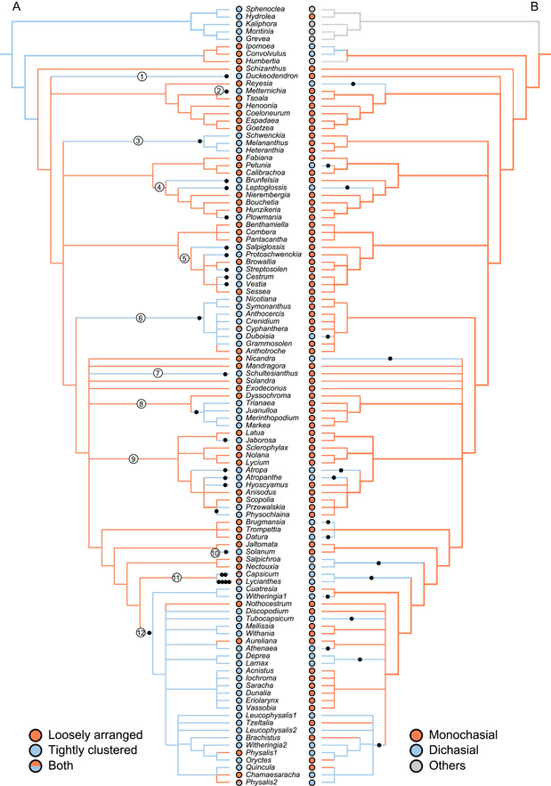
The ancestral state reconstruction (ASR) summary of Solanaceae inflorescence structures on a genus‐level phylogeny. The left side shows the evolutionary transitions between loosely arranged (orange) and tightly clustered (blue) inflorescences. These results are summarized from the ASR based on maximum likelihood (ML) inferences on a species‐level phylogeny (Appendix S5). The black dots represent 27 independent evolutionary transitions from ancestral loosely arranged inflorescences to tightly clustered inflorescences, while the numbers along the branches indicate the clades where the transitions occurred. The right side shows the evolutionary transitions between the monochasial (orange) and dichasial (blue) branching patterns of inflorescences. The analysis was based on the ASR using ML inferences on a genus‐level phylogeny (File S2). Each black dot indicates a single transition from monochasial to dichasial branching patterns. Subsequent reversals to loosely arranged or monochasial inflorescences are not indicated.

We tested the evolutionary relationships between monochasial and dichasial inflorescences at the genus level. The ASR results based on MK1 model suggested that the ancestral state of Solanaceae as a whole is the monochasial pattern (support 98.5%, Appendix S9). Dichasial inflorescences evolved 16 times independently in different lineages (Figure 3B), and was then lost in four genera, i.e., Tzeltalia E. Estrada & M. Martínez, Brachistus Miers, Oryctes S. Watson, and Quincula Raf. (Figure 3B).

Morphological modifications of inflorescences in Solanaceae

The 2D models based on our observations of the inflorescences allowed us to illustrate the organs in each repeating unit of inflorescences and to understand the evolutionary modifications of the basic structures (Figure 4; Appendices S10–S31). We found that the basic unit that makes up Solanaceae inflorescences usually contains five components. These five components are arranged along the inflorescence axis and include two FPPs, each with an axillary bud, and one terminal structure, the flower (Figure 4B). This basic inflorescence unit repeats itself, starting just below the previous flower (Figure 4B).

Figure 4.

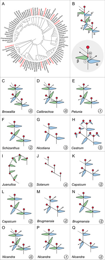
Inflorescence branching patterns observed in the 12 species studied. The phylogenetic positions of the examined species are indicated in a genus‐level tree (A). The basic unit of the inflorescence (B) in Solanaceae comprises five components, including two flower‐preceding prophylls (FPPs), the axillary shoots associated with the two FPPs, and a terminal flower, at three nodes. At each of the first two nodes, there is a FPP and an axillary shoot, while at the third node immediately below the terminal flower the next repeating unit of the inflorescence develops and continues the inflorescence growth. This structure is inferred from an analysis of the inflorescences of Browallia speciosa (C), Calibrachoa elegans (D), Petunia ×hybrida (E), Schizanthus grahamii (F), Nicotiana obtusifolia and Nicotiana tabacum (G), Cestrum aurantiacum (H), Juanulloa mexicana (I), Solanum lycopersicum (J), Capsicum annuum (K, L), Brugmansia suaveolens (M, N), and Nicandra physalodes (O–Q). The evolutionary transitions that give rise to the diverse inflorescences in Solanaceae include the losses or reduction of FPPs, axillary shoots, internodes, and flower pedicels (C–Q). The oval shapes in blue and green represent the α‐ and β‐FPPs developing along the flowering branch that usually point to the sideward and upward, respectively, relative to the flat zigzag inflorescence plane (also see 3D modeling results). The arrows indicate axillary vegetative shoots. The arrows with a circle head indicate the axillary shoots developed inflorescence branches. The dotted lines indicate the continuation of the inflorescences. In (B), the blue and red sticks represent the internodes between nodes I and II, and nodes II and III, respectively. The red circles represent flowers. The numbers in the circles (C–Q) indicate reduction in the number of structures of the inflorescence unit from that of the basic structure (B). The phylogenetic tree was modified based on Olmstead et al. (2008).

In Bro. speciosa, the repeating unit of the inflorescence contains all five components, including a FPP and an axillary shoot at both the first and second nodes, and a flower (Figure 4B, C; Appendices S10, S22). The flower represents the termination of the apical meristem of the shoot from the developmental perspective; it is not in the axillary position. For 3D display, the FPP that develops at the first node of the repeating inflorescence units is horizontal/lateral relative to the flat zigzagging inflorescence plane, while the FPP at the second node is upward‐pointing and is held vertical relative to the inflorescence plane (Figure 4B,C; for 3D model, see Appendix S32). To distinguish the two FPPs in the diagrams, we called the FPP at the first node α‐FPP and colored it blue, and we called the FPP at the second node β‐FPP and colored it green. The importance of distinguishing between the FPPs growing at nodes I and II is that they represent serially homologous organs. The examples from the other solanaceous species presented below show that when these leaves are lost during evolution, they are always lost as a set; that is, either all α‐FPPs, or all β‐FPPs are lost. The inflorescence continues by the growth of the axis from a position just below the flower initiated (Figure 4C, see below). The continuation of the zigzag pattern of inflorescence branching results from the repeated growth of the inflorescence unit from alternate sides of the inflorescence axis.

We found that the inflorescence units throughout Solanaceae are modifications of this basic unit. For all the other examined species, internodes are usually highly reduced, which gives the impression that all components of each unit grow at the same node. For example, Cal. elegans has the same five components in its inflorescence unit as does Bro. speciosa (Figure 4D; Appendix S11, S23, S33), while the other examined species have a reduced number of components (Figure 4). We noticed that the younger repeating units of Bro. speciosa usually have highly reduced internodes, while longer internodes are evident in the older repeating units (Figure 4B, C; Appendices S10, S22, S32).

Pet. ×hybrida has no shoot growing from the axil of the β‐FPP, the upward‐pointing FPP (Figure 4E; Appendices S12, S24, S34), while the vegetative bud growing in the axil of the α‐FPP pointing outward is usually suppressed until after flowering. In Sch. grahamii, both FPPs lack axillary shoots (Figure 4F; Appendices S13, S25, S35), while in Nicotiana species, Ces. aurantiacum and Jua. mexicana, three of the five components, including the two axillary shoots and one FPP, are missing in each repeating unit (Figure 4G–I; Appendices S14–S17, S26–S28, [Link], [Link], [Link], [Link]). The two Nicotiana species sampled, i.e., Nico. obtusifolia and Nico. tabacum, similarly continue the inflorescence by adding repeating units (Figure 4G; Appendices S14–S15, S26, S36–S37). The repeating unit of Ces. aurantiacum is highly modified and distinct from those of the other taxa illustrated in Figure 4. Here the inflorescence unit is a three‐flowered cyme, which is further aggregated into a panicle inflorescence (Figure 4H; Appendices S16, S27, S38). Each inflorescence unit of Jua. mexicana consists of only one flower and one FPP, and the whole inflorescence is helicoid (Figure 4I; Appendices S17, S28, S39). In Sol. lycopersicum, each inflorescence unit is made up of just a single flower, four of five components of the inflorescence unit including all FPPs and axillary shoots being lost (Figure 4J; Appendices S18, S29, S40).

We also found that in some solanaceous species the development of the inflorescence patterns can be plastic. Thus, in Cap. annuum, each inflorescence unit lacks two components compared to the basic model (Figure 4K, L; Appendices S19, S30, S41). Interestingly, exactly which two components are missing depends on the stage of inflorescence development. At an early stage, one FPP and the axillary bud associated with this FPP are missing (Figure 4K; Appendices S30, S41). The inflorescence branching is dichasial at this stage (Figure 4K). At a later stage, both FPPs remain but both axillary shoots are missing, and the inflorescence branching is monochasial (Figure 4L). The inflorescence of Bru. suaveolens is similar to that of Cap. annuum (Figures 4M, 4N; Appendices S20, S31, S42). For Nica. physalodes, more components are again missing at the later stages of inflorescence growth. We observed three patterns for the same individual, including an inflorescence unit possessing all five components at an early stage of inflorescence development (Figure 4O; Appendix S21), inflorescence units like those in Pet. ×hybrida at the mid‐stage (Figures 4E, 4P), and inflorescence units like those in Cap. annuum and Bru. suaveolens (Figures 4K, 4M) at a late stage of inflorescence development (Figure 4Q).

In Solanaceae, vegetative growth, including that of the SAM in the embryo and of the lateral axillary shoots, is monopodial. The branching pattern switches to sympodial when reproductive growth begins (also see Huber, 1980). The makeup of each inflorescence unit from vegetative to reproductive growth along the primary inflorescence axis is usually conserved within species (Figure 5). The first inflorescence unit represents the initial transition from vegetative to reproductive growth (Figure 5: 1°). The following units (Figure 5: 2° and above) represent those developing from the primary inflorescence axis. The composition of each unit is usually conserved along the primary axis (Figure 5), but when variable, the variations are also indicated (Figure 5F,G). In several species, including Sch. grahamii (Figure 5A), Pet. ×hybrida (Figure 5B), Ces. aurantiacum (Figure 5C) and Nicotiana species (Figure 5D, E), the first inflorescence unit that marks the transition from vegetative to reproductive growth is different from the others. Thus, the first inflorescence unit of Sch. grahamii has a phyllome, an axillary shoot, and a flower, but there are the paired FPPs and a flower in the other inflorescence units (Figure 5A). In Pet. ×hybrida, only the axillary bud of the first inflorescence unit develops immediately as another inflorescence, but those on the following units grow a vegetative shoot (Figure 5B). The two species of Nicotiana have different patterns at the first flowering node. In Nico. obtusifolia, the first inflorescence unit has three inflorescence axes at this node (Figure 5D), while the first unit of Nico. tabacum has two inflorescence axes but no flower there (Figure 5E). Finally, as mentioned, in Cap. annuum (Figure 5F), Bru. suaveolens (Figure 5F), and Nica. physalodes (Figure 7G), the first few inflorescence units differ from the later inflorescence units. In particular, the first several inflorescence units of Cap. annuum and Bru. suaveolens show a dichasial pattern (Figure 5F), but the inflorescence branches at a later stage of development are monochasial (Figure 5F). Similarly, in Nica. physalodes, the first two to three inflorescence units are dichasial, although one of the inflorescence branches usually grows several phyllomes before flowering. This is unlike Cap. annuum and Bru. suaveolens where both inflorescence branches flower in a symmetrical pattern, but the one (original inflorescence axis) precedes the other (axillary branch). In the other species observed, i.e., Bro. speciosa, Cal. elegans, Jua. mexicana, and Sol. lycopersicum, the repeating units throughout the inflorescences are identical.

Figure 5.

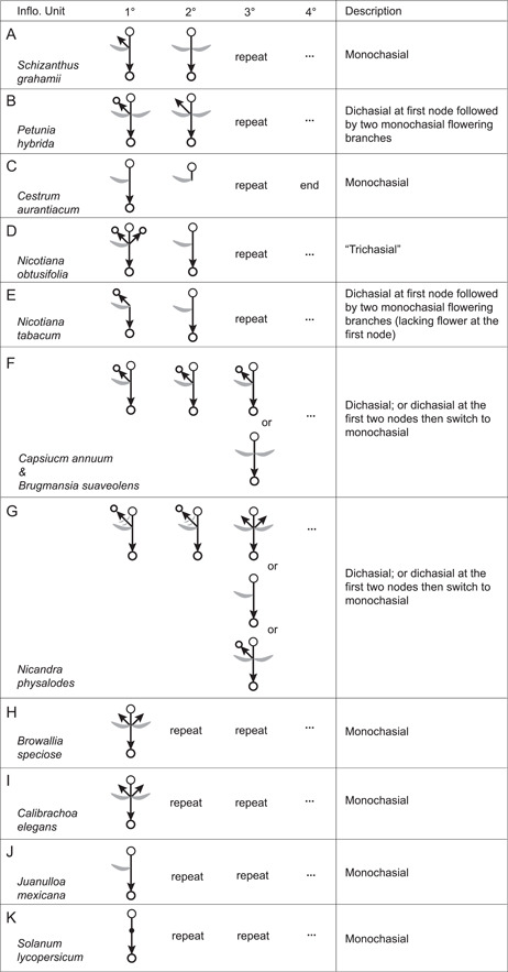
Inflorescence growth modes in the studied species. The circle with a stick indicates the flower; the arrow alone indicates the vegetative shoot; the arrow with a circle head indicates the inflorescence; the crescent in grey shows the leaf. “1°, 2°, 3°, 4°” indicate branching orders, “repeat” indicates that the inflorescence unit repeats as the previous unit, “…” that the structure of the last node continues indefinitely, and “end” that the inflorescence ends at that node.

Figure 7.

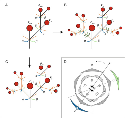
A new model for the evolution of scorpioid‐like cymes (A–C) and a modified model of floral zygomorphy in Solanaceae (D). (A–C) Based on the ancestral state reconstruction (ASR) and morphological studies, the most recent common ancestor (MRCA) of Solanaceae had a monochasial‐like cyme (A), and dichasial‐like cymes (B, C) are derived from the modification of such a cyme, one of the two axillary meristems (orange arrows) growing as an inflorescence branch, which is always smaller in size compared with the original inflorescence axis (black branches) because it develops later. Thus, in Nicandra physalodes (B), the branch developed from the axillary shoot always bore several leaves before terminating in a flower, while in Capsicum annuum and Brugmansia suaveolens (C), the branch developed from the axillary shoot flowered immediately. Reduction or abortion of the other axillary shoot and associated leaf‐like organ are observed, with their rudiments still discernible (Figure 6). The flowers along three subsequent orders are F _n−1, F _n , and F _n+1. (B) is based on Nicandra physalodes and illustrated from the first branching order; therefore, for (B), n = 2. (D) Model of floral zygomorphy in Solanaceae. The positions of the two flower‐preceding prophylls (FPPs) relative to the rest of the flower and the two dorsal and single ventral stamens that may become modified or aborted are shown. One of the dorsal stamens is on the inflorescence axis (IA)‐ovary plane, the median plane, indicated by a dashed gray line, the other is on the β‐FPP (in green)‐ovary plane, indicated by a solid gray line. The ventral stamen is on the α‐FPP (in blue)‐ovary plane, the plane of floral symmetry, and shown as a solid black line with the arrowhead pointing to the ventral side of the flower. The solid‐line circle indicates the IA; dotted‐line circles represent the growth of the axillary buds of the FPPs.

Rudimentary organs support the hypothesis of a modified basic structure

Our morphological study revealed rudimentary organs in the inflorescence development of Cap. annuum and Nica. physalodes (Figure 6). Both have rudimentary components in each inflorescence unit (Figure 6B–G). Of the two aborted organs in an inflorescence unit of Cap. annuum, one has a phyllome shape (Figure 6A‐3, C‐3), and the other is like an undeveloped bud (Figure 6A‐4, C‐4; note, there is the polymorphism of inflorescence unit structure described above; Figure 6B and C correspond to the inflorescence structure in Figure 4K). For Nica. physalodes, the growth of one axillary bud is arrested but the bud is still discernable (Figure 6A‐4, D‐G‐4). The dichasial branching of the Nica. physalodes inflorescence results from the continuation of the inflorescence on one side (Figure 6A‐IA, D‐G‐IA) and the development of the axillary bud on the other side (Figure 6A‐2, D‐G‐2). Of the two flowering branches of the dichotomizing structure in Nica. physalodes, one clearly precedes the other. The one that develops first represents the continuation of the inflorescence since it immediately repeats the inflorescence unit, while the other branch grows several leaves before flowering suggesting that it was initially a vegetative shoot.

Figure 6.

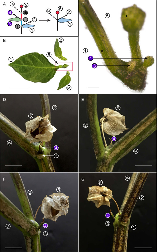
Rudimentary organs on inflorescences of Capsicum annuum and Nicandra physalodes. These rudimentary structures support the hypothesis that modification of the basic inflorescence unit gives rise to the inflorescence structures of Capsicum annuum and Nicandra physalodes (summarized in A). The five components of an inflorescence unit, including two flower‐preceding prophylls (FPPs) (1 and 3), the axillary shoots associated with the two FPPs (2 and 4, respectively), and a terminal flower (5), grow along the inflorescence axis (IA). In Capsicum annuum, one FPP (3) and the axillary shoot associated with this FPP (4) are aborted (B, C). A close up (C) of the boxed region in (B) shows the rudimentary organs (3 and 4). Similarly, in the first inflorescence unit of Nicandra physalodes, an aborted axillary shoot (4) is associated with a leaf represented by a leaf scar (D–G, shown from different angles). The other leaf (G‐1) is indicated by a leaf scar subtending the axillary shoot (G‐2). In contrast, no leaf scar was found subtending the continuation of the inflorescence (F‐IA), suggesting the different origins of these seemingly identical bifurcating branches. Scale bars: B, D–F, G = 1 cm; C = 0.1 cm.

Floral display along the inflorescence of Solanaceae

The 3D model allows us to identify the spatial position of the inflorescence axis and FPPs associated with the flower in relationship to the zygomorphic flower display. The 3D model of Bro. speciosa indicates that the α‐FPP associated with the zygomorphic flower is positioned at the ventral position between the two ventral petals (Appendix S32, marked in blue), while the β‐FPP associated with the zygomorphic flower (Appendix S32, marked in green) and also the inflorescence axis (Appendix S32, labeled in pink) is located between the dorsal and the lateral petals on the left and right, respectively (or vice versa for the flower growing at the alternate position of the inflorescence axis). Axillary shoots develop in association with each of these two FPPs. The inflorescence axis and FPPs of Sch. grahamii have a similar position spatially like those of Bro. speciosa, but there are no shoots axillary to the two FPPs (Appendix S35).

The 3D models of the inflorescences of Cal. elegans and Pet. ×hybrida are similar (Appendix S33 and S34). In these two species, the apparent orientation of the two FPPs relative to the flower are somewhat different from Bro. speciosa and Sch. grahamii primarily due to the bending of the long pedicel of the flower in the first two species.

Nico. obtusifolia (Appendix S36), Nico. tabacum (Appendix S37), Bru. suaveolens (Appendix S42), Cap. annuum (Appendix S41), Ces. aurantiacum (Appendix S38), and Jua. mexicana (Appendix S39) have only a single FPP associated with each inflorescence unit. In the first four species, this FPP is always on the side of the inflorescence axis opposite to where the flower develops. However, in Ces. aurantiacum and Jua. mexicana, both the FPP and the flower are borne on the same side of the axis (Appendices S38, S39). These differences may suggest that the FPPs on the inflorescences in the two groups of species are not homologous. Solanum lycopersicum has the most reduced inflorescence (Appendix S40); however, its inflorescence axis has the same zigzag pattern as seen in all the other solanaceous species.

DISCUSSION

The evolution of flower arrangement on inflorescences in Solanaceae

The evolution of inflorescences has been thought to be driven by both pollinator and the climate (Stebbins, 1973; Borchert, 1983; Wiens and Donoghue, 2004). The change from loosely arranged inflorescences with extended flowering periods to tightly clustered inflorescences with synchronized flowering was thought to be an adaptation to a shortened growing season (Stebbins, 1973; Wyatt, 1982). For example, in groups with both types of inflorescences, such as Scrophulariaceae, Phrymaceae, Fabaceae, Campanulaceae, and Caprifoliaceae‐Valerianoideae, species with loosely arranged inflorescences usually occur in moist habitats and have an extended flowering season, while species having inflorescences with tightly clustered flowers are more likely to be found in either alpine or xeric habitats and have a short flowering season (Stebbins, 1973; Borchert, 1983). Inflorescences with clustered flowers likely enable the plants to produce flowers and seeds in a shorter favorable period to avoid harsh environmental conditions such as cold and drought (Stebbins, 1973; Borchert, 1983).

Here we looked at the evolutionary transitions from loosely arranged to tightly clustered inflorescences in Solanaceae. Based on our ASRs, the MRCA of Solanaceae had a loosely arranged inflorescence, while tightly clustered inflorescences are derived (Figure 3A). Solanaceae are an angiosperm group that have experienced numerous ecological shifts during their diversification, as when moving from the tropics to temperate regions and cool climates (Olmstead, 2013). Based on the molecular phylogeny and fossil evidence, the crown‐group age of Solanaceae is estimated to be ca. 60–30 million years ago (Mya) (summarized by Stevens [2001 onward]; also see the discovery of early Eocene fossils [52.5 Mya] of Physalis infinemundi Wilf and Physalis hunickenii Deanna, Wilf & Gandolfo from Argentina [Wilf et al., 2017; Deanna et al., 2020]), and much of the later radiation of the group appears to be primarily centered in South America (Olmstead, 2013; Dupin et al., 2017). Sixteen of the 19 recognized clades are represented in the New World, and all of these 16 clades have South American representatives (Olmstead, 2013). In South America, the uplift of the Andes has continued since the Paleogene (ca. 30 Mya) (Gregory‐Wodzicki, 2000; Hoorn et al., 2010), albeit at different rates, and has been a major force in creating new valleys, slopes, and highlands. These newly established habitats provided a unique microclimate for the flora to adapt and diversify (Ghosh et al., 2006; Garzione et al., 2008). Species of Solanaceae can be found in virtually all terrestrial ecosystems in South America, further evidence of a history that has involved numerous ecological shifts during their diversification (Olmstead, 2013). Most of the larger clades within the family (e.g., Nicotianoideae, clade 6; Solaneae, clade 10; Capsiceae, clade 11; and Physaleae, clade 12 in Figure 3A) are significantly represented in both xeric and mesic ecological zones and occupy broad latitudinal ranges, reaching into cool temperate climates in South America (Olmstead et al., 2008; Olmstead, 2013; Dupin et al., 2017). In Old World, several genera (e.g., Lycianthes within clade 11 and Physalis within clade 12 in Figure 3A) are distributed broadly from the tropics to high latitudes (Olmstead et al., 2008; Olmstead, 2013). Furthermore, several lineages (e.g., Nicotianoideae, clade 6 in Figure 3A; Hyoscyameae, partial clade 9 in Figure 3A; and Physalis in clade 12 in Figure 3A), are diverse in relatively arid and/or cool habitats today (Olmstead, 2013), which may reflect the global trend toward increasing aridity and the shrinking of tropical forests since the late Miocene (Willis and McElwain, 2014; Torsvik and Cocks, 2017). Our results indicate that there were multiple evolutionary transitions between loosely arranged and tightly clustered inflorescences within all these clades (Figure 3A; Appendix S8). It would be interesting to test whether adaptation to novel ecological niches and the shifts and diversification of inflorescence structure in Solanaceae are associated.

A novel mechanism underlying the evolution of the scorpioid cyme in Solanaceae

In the existing model, the scorpioid cyme originated from a compound dichasium through the alternate reduction of one side of the dichasial branches, resulting in a monochasial branching pattern (Figure 1A–C; modified from Stebbins, 1973, 1974). Some scorpioid cyme structures fit into this model perfectly, such as in Boraginaceae (Buys and Hilger, 2003), Juncus lamprocarpus Rchb. (Eichler, 1875–1878), and Pentaphragma Wall. ex G. Don (Stevens, 2001 onward). Eichler (1875–1878) tried to fit the evolution of scorpioid cymes in Solanaceae into this model and also thought that monochasial evolved from dichasial branching patterns here. The challenge for Eichler was that the Solanaceae scorpioid cymes often have two phyllomes associated with each flower instead a single one based on the classical model (Figure 1A–C). To explain the extra phyllome, Eichler (1875–1878) proposed that one of the two axillary shoots of the basic dichasial inflorescence aborts, but a leaf of a lower node persists, hence resulting in these two phyllomes being associated with a flower (reviewed by Child, 1979) (Appendix S43). Danert (1958) and Child (1979) adopted the phenomenon, recaulescence, the fusion of the leaf stalk to the branch, and used the opposite process to explain how the leaf along axillary shoots can become associated with the previous branching order. Eichler's model of inflorescence evolution in Solanaceae was later adopted by several researchers (Danert, 1958, 1967; Troll, 1969; Child, 1979).

Eichler's model, however, was not supported by any anatomical evidence. The anatomical work by Fattah (1955) has shown that the extra leaf in Eichler's model is an appendage just like a regular leaf, and there is also no evidence that it is adnate to or shifted from a lateral branch. Most importantly, our ASR results indicated that the inflorescence structure of the MRCA of Solanaceae is a monochasium and that the dichasium is derived, an evolutionary trajectory of the origin of the scorpioid cyme opposite to that of the standard model (Figure 3B).

To better understand Solanaceae inflorescence evolution, we characterized the components that make up the basic inflorescence unit and proposed a model made up of three nodes and five components (Figure 4B, Appendix S32). Notably, we observed that some species, such as Bro. speciosa, possess all five components and have elongated internodes between the three nodes in each inflorescence unit (Figure 4B, C). The other inflorescence types of Solanaceae represent a modification of this basic structure (Figure 4D–Q). Thus, the reduction of FPPs at nodes I or II usually occurs together; thus, all α‐FPPs at node I are lost in Jua. mexicana, and all β‐FPPs at node II are lost in Nicotiana species (Figure 4). Some inflorescences like those of Sol. lycopersicum have completely lost all FPPs along the inflorescence. A similar loss of phyllomes is not uncommon elsewhere. For example, inflorescences of most Brassicaceae and several lineages of Alismatales lack FSBs (Hagemann, 1963; Prenner, 2004).

The origin of the dichasium from the monochasium in Solanaceae represents the continued growth of an axillary shoot, which pairs with the continued growth of the original inflorescence branch (Figure 7A–C). This axillary shoot usually grows slower than the inflorescence branch, as in Cap. annuum and Bru. suaveolens (Figure 7C), which independently evolved a similar type of dichasium from a monochasium, or it produces several vegetative nodes before flowering, as in Nica. physalodes (Figure 7B). These observations further support our hypothesis that it is the modification of the components of the basic inflorescence unit, including the FPPs and the axillary shoots, that gives rise to inflorescence diversity in Solanaceae.

Despite a general agreement that Solanaceae inflorescences have cymose branching patterns, Solanaceae inflorescences have been interpreted in various ways (reviewed by Huber, 1980). The challenges have been interrelating the diverse inflorescence topologies while lacking a firm phylogenetic framework. Inflorescences of Solanaceae have been described as thyrsoids, that is, determinate thyrses (Danert, 1958; Endress, 2010). For thyrsoids, the main axis (first‐order) is racemose, but it is ultimately terminated by a flower, and the cymose partial inflorescences make up the second‐ and higher‐order axes. Thus, the main axis of a thyrsoid grows an unlimited number of second‐order branches. However, in Solanaceae, we show that the first‐order axis never has more than two second‐order axes and never has more than two phyllomes (also see Huber, 1980). Therefore, the first‐order Solanaceae inflorescence axis is also cymose, which does not strictly fit the thyrsoid “type”.

Comparison of the known ontogeny of the cyme further supports the idea that the Solanaceae inflorescences are not typical cymes. Ontogenetic studies indicate that cymes originate from floral unit meristems (FUMs) and like floral meristems (FMs) are determinate (Claßen‐Bockhoff and Bull‐Hereñu, 2013). However, unlike FMs that are usually completely differentiated when forming floral organs, cymose FUMs have a terminal flower and one or two lateral parts maintaining meristematic activity. Each of the lateral parts can give rise to a subtending bract and an axillary meristem from which further di‐ and/or monochasial branching may continue (Claßen‐Bockhoff and Bull‐Hereñu, 2013). The basic structure of the Solanaceous inflorescence is not that of such a cyme. In a Solanaceae cyme‐like structure, the FUM‐like meristem typically splits into a terminal flower and three lateral parts, i.e., two meristems, each subtended by a phyllome, and one FUM‐like meristem without an associated phyllome (Figure 7D). Then the FUM‐like meristem repeats the process. In the loosely arranged flowering branches in Solanaceae, the FUM‐like meristem periodically acts like a vegetative meristem (VM) and produces two foliage leaves—their associated axillary meristems have delayed growth—and then changes into a FUM that produces a terminal flower and a meristem that continues the pattern. In tightly arranged inflorescences in Solanaceae, the VM period is suppressed, and cymes are developed from the FUM throughout the inflorescence development. Thus, the Solanum inflorescence fits the FUM model of a cyme development, while that of Petunia does not (but also see Zhang and Elomaa, 2021). Our detailed morphological analyses of inflorescence development within a phylogenetic framework, therefore, have helped us to discover a novel mechanism underlying the evolution of the cyme‐like inflorescence in Solanaceae.

A modified model for understanding the development of floral zygomorphy in Solanaceae

The development of floral zygomorphy in angiosperms was thought to be associated with flowers that grow at the axillary position; that is, zygomorphic flowers are usually axillary, while actinomorphic flowers are often terminal (Coen and Nugent, 1994; Degtjareva and Sokoloff, 2012). Many zygomorphic‐flowered species establish floral zygomorphy along the median plane, while in others, zygomorphy is established along an oblique plane (see summary in Bukhari et al., 2017). In dicotyledonous plants, the FPPs usually occur in pairs and are inserted in a more or less transverse position (opposite or alternate) relative to the median plane (Weberling, 1989).

We demonstrated how the floral organs of the zygomorphic flower are relatively arranged along the inflorescence axis with the FPPs in Solanaceae based on 3D models. We studied the zygomorphic flowers of Sch. grahamii, Bro. speciosa, Cal. elegans, and Pet. ×hybrida and found that the two FPPs do not have the arrangement just mentioned as being common in dicotyledonous plants, they are not both transverse (Appendix S32‐S35). A model based on a complete inflorescence unit, as in Bro. speciosa, shows the relative positions of two acropetally developed FPPs (a vegetative shoot grows from the axil of each) and the inflorescence axis (IA) in relationship to the terminal flower using a floral diagram (Figure 7D). One dorsal stamen is on the median plane defined by the inflorescence axis and the flower center (Figure 7D, the dotted line), while the other dorsal stamen is on a plane defined by the β‐FPP and its associated axillary bud and the flower center (Figure 7D, the gray line); it is the single ventral stamen and the α‐FPP and its associated axillary bud that lie along the plane of floral symmetry (Figure 7D, the black arrow). The first two planes just mentioned are arranged obliquely and symmetrically relative to the plane of floral symmetry (Figure 7D). Indeed, floral zygomorphy of Solanaceae is oblique, being 36° off the median plane (Wydler, 1866; Eichler, 1875–1878; Robyns, 1931), and we show how this relates to the unusual arrangement of the paired FPPs in Solanaceae. The protracted disputes about the development of floral zygomorphy in Solanaceae are mainly because of a mistake in interpreting the nature and position of the FPPs associated with the flower (Figure 2; Wydler, 1866; Eichler, 1875–1878; Grau and Grönbach, 1984; Cocucci, 1989; Ampornpan and Armstrong, 2002).

Floral zygomorphy in Solanaceae is unique from both the evolutionary and developmental perspectives (this study; Robyns, 1931; Cocucci, 1989; Knapp, 2002; Zhang et al., 2017). Unlike the gain or loss of floral zygomorphy simultaneously in both androecium and corolla seen in many plant groups (Endress, 1999; Citerne et al., 2010), Solanaceae commonly show zygomorphy in the androecium but rarely in the corolla (but see also Melastomataceae [Varassin et al., 2008] and Polemoniaceae [Schönenberger, 2009]). We recently demonstrated that the floral zygomorphy of Solanaceae likely evolved in androecium and corolla along separate evolutionary trajectories (Zhang et al., 2017). Thus, the flower of the most recent common ancestor of Solanaceae has a zygomorphic androecium but actinomorphic corolla, and multiple losses of floral zygomorphy in the androecium and multiple gains of zygomorphy in the corolla underlie the homoplastic patterns of this trait in the family (Zhang et al., 2017). Here we show that the development of floral zygomorphy is also unique in Solanaceae. Usually the single (or three) dorsal stamen(s) of a zygomorphic flower like Antirrhinum majus L. abort (Eichler, 1875; Luo et al., 1996). In A. majus, the zygomorphic flowers are axillary along a single inflorescence axis and is each subtended by an FSB (Luo et al., 1996); the dorsal stamen is staminodial. However, in Solanaceae, both the two dorsal and one ventral (to emphasize: dorsal and ventral is in the context of the plane of symmetry of the flowers) stamens are modified or aborted (Robyns, 1931; Cocucci, 1995; Knapp, 2002; also see Endress, 1999; and examples in angiosperms reviewed by Bukhari et al., 2017). The inflorescence bearing the flowers was thought to influence floral symmetry, particularly in early development (Tucker et al., 1993; Endress, 1999), a speculation based on the observation that actinomorphic flowers of some species are strongly zygomorphic early in development, especially in spikes or racemes. It was believed that the shoot and FSB as two polar areas influenced the symmetry of the axillary flower. A recent developmental simulation study implied that the dorsal‐ventral inhibitory field primarily regulates floral symmetry and can generate floral symmetry diversity (Nakagawa et al., 2020). We have shown that in Solanaceae, the flower is frequently associated with three axes, one established by the inflorescence axis and two by the axillary shoots growing from the axils of the two FPPs (Figure 7D). Interestingly, each of the three axes is on the same radius as one of the three aborted/modified stamens. This work lays the foundation for a renewed understanding of the evolution and the developmental genetics of zygomorphic flowers in the Solanaceae.

CONCLUSIONS

The most recent common ancestor of Solanaceae had a loosely arranged monochasial cyme‐like inflorescence and later independently evolved tightly clustered and dichasial cyme‐like inflorescences many times within the family. Our analyses indicate that this ancestral scorpioid cyme‐like morphology does not result from parallel evolution of the known mechanism of scorpioid inflorescence development but by convergent evolution through an undescribed developmental process. In Solanaceae, dichasial cyme‐like structures evolved from monochasial cyme‐like forms. Interestingly, this evolutionary transition from monochasial to dichasial cyme has not been observed elsewhere in angiosperms, although the reverse sequence is typical (Endress, 2010). Due to the unique inflorescence branching pattern, the flower is not situated between an inflorescence axis and an FSB, and the two FPPs associated with the flower are not positioned like the regular paired FPPs positioned transversely as seen in dicotyledonous plants. Furthermore, many Solanaceae have vegetative shoots in the axils of these FPPs. Revealing the inflorescence evolution and development patterns helps us confirm that the plane of symmetry of the zygomorphic Solanaceae flower is at 36° from the median plane and that it cuts through the ventral α‐FPP, the inflorescence axis (on the median plane) and the β‐FPP being dorsally positioned and symmetrical to the plane of floral symmetry. We suggest in this comparative study that new developmental mechanisms are needed to explain the evolution of morphological diversity in Solanaceae.

AUTHOR CONTRIBUTIONS

W.Z. conceived and planned the study. J.Z. and W.Z. executed data collection. J.Z. conducted the analyses. W.Z., J.Z., and P.F.S. wrote the manuscript. All authors contributed to the drafts and approved the final publication.

Supporting information

Appendix S1. The description of inflorescence structure and branching pattern of Solanaceae and its outgroups at species‐ and genus‐level as taken from the literature. For inflorescence structure, 0 represents a loosely arranged inflorescence; 1 represents a densely clustered inflorescence; question marks indicate the character state is unclear. For branching pattern, 0 represents a monochasial branching pattern; 1 represents a dichasial branching pattern; 2 represents other branching patterns exhibited in the outgroups.

Appendix S2. Voucher information for this study.

Appendix S3. The comparison of the models used for ancestral state reconstructions (ASRs) using maximum likelihood (ML) method. Notes: Likelihood ratio (LR) tests were calculated using LR = 2 × (Lh2parameter − Lh1parameter). Lh stands for the log likelihood values. The P‐value was calculated by chi‐square test with df = 1. Character states are 0 = loosely arranged inflorescence; 1 = densely clustered inflorescence.

Appendix S4. The statistics of ancestral state reconstruction (ASR) results inferred by the Bayesian approach. Character states are 0 = loosely arranged inflorescence; 1 = densely clustered inflorescence; question mark = character state unclear.

Appendix S5. Species‐level ancestral state reconstructions (ASRs) of inflorescence structures in Solanaceae with outgroups based on the maximum likelihood (ML) inference. Loosely arranged inflorescences and tightly clustered inflorescences are marked with pink and green, respectively, in the pie charts. The areas occupied by particular colors in the pie charts indicates the likelihood of the character states at each internode.

Appendix S6. The original Mesquite (Maddison and Maddison, 2017) file for the maximum likelihood (ML) ancestral state reconstruction (ASR) inference on a species‐level phylogeny.

Appendix S7. Species‐level ancestral state reconstructions (ASRs) of inflorescence structure in Solanaceae and outgroups based on the Bayesian approach. Loosely arranged inflorescences and tightly clustered inflorescences are marked with pink and green in the pie charts. The areas occupied by particular colors in the pie charts shows the likelihood of the character states at each internode. Missing data are black.

Appendix S8. A summary of clades where shifts from loosely arranged (0) to densely clustered (1) inflorescences occurred. Our analyses identified 27 shifts from the ancestral loosely arranged inflorescence found in the most recent common ancestor (MRCA) of Solanaceae to densely clustered inflorescences. Densely clustered inflorescences were also lost and regained eight times in two clades, i.e., Capsiceae and Physaleae. The names of the subgenera are based on Olmstead et al. (2008).

Appendix S9. The original Mesquite (Maddison and Maddison, 2017) file for the maximum likelihood (ML) ancestral state reconstruction (ASR) inference of branching pattern on a genera‐level phylogeny.

Appendix S10. Schemes of the inflorescence structures of Browallia speciosa observed from three different branches of three individuals. The blue oval represents the α‐flower‐preceding prophyll (α‐FPP) that is at the first node of the repeating inflorescence unit and is horizontal relative to the plane that the zigzag inflorescence axis defines; the light green oval represents the β‐FPP that is at the second node and is upward and vertical relative to the inflorescence plane. The white dotted line marks the single dorsal petal of zygomorphic flowers. The black dotted line represents the continuation of the inflorescence. The black arrow represents the vegetative shoot. The brown stick represents the stem that grows before the transition to the reproductive growth. The red circles represent old or unopened flowers.

Appendix S11. Schemes of the inflorescence structures of Calibrachoa elegans observed from three different branches of three individuals. The blue oval represents the α‐flower‐preceding prophyll (α‐FPP) that grows at the first node of the repeating inflorescence unit and is horizontal relative to the plane that the zigzag inflorescence axis defines; the light green oval shape represents the β‐FPP that grows at the second node and is upward and vertically positioned relative to the inflorescence plane. The white dotted line marks the single dorsal petal of zygomorphic flowers. The black dotted line represents the continuation of the inflorescence. The black arrow represents the vegetative shoot. The brown stick represents the stem that grows before the transition to reproductive growth.

Appendix S12. Schemes of the inflorescence structures of Petunia ×hybrida observed from four different branches of three individuals. The blue oval represents the α‐flower‐preceding prophyll (α‐FPP) that grows at the first node of the repeating inflorescence unit and is horizontal relative to the plane that the zigzag inflorescence axis defines; the light green oval represents the β‐FPP that grows at the second node and is upward and vertically positioned relative to the inflorescence plane. The white dotted line marks the single dorsal petal of zygomorphic flowers. The black dotted line represents the continuation of the inflorescence. The black arrow represents the vegetative shoot. The brown stick represents the stem that grows before the transition to reproductive growth.

Appendix S13. Schemes of the inflorescence structures of Schizanthus grahamii observed from four different branches of two individuals. The oval shape with dark green represents the first phyllome that subtends the whole inflorescence. The blue oval represents the α‐flower‐preceding prophyll (α‐FPP) that grows at the first node of the repeating inflorescence unit and is horizontal relative to the plane that the zigzag inflorescence axis defines; the light green oval represents the β‐FPP that grows at the second node and is upward and vertically positioned relative to the inflorescence plane. The white dotted line marks the single dorsal petal of zygomorphic flowers. The black dotted line represents the continuation of the inflorescence. The black arrow represents the vegetative shoot. The brown stick represents the stem that grows before the transition to reproductive growth.

Appendix S14. Schemes of the inflorescence structures of Nicotiana obtusifolia observed from three different branches of three individuals. The blue oval shape represents the flower‐preceding prophyll (FPP) that usually alternates with the flower; the red circle represents the flower. The black dotted line represents the continuation of the inflorescence. The brown stick represents the stem that grows before the transition to reproductive growth.

Appendix S15. Schemes of the inflorescence structures of Nicotiana tabacum observed from three different branches of three individuals. The blue oval shape represents the flower‐preceding prophyll (FPP) that usually alternates with the flower; the red circle represents the flower. The black dotted line represents the continuation of the inflorescence. The brown stick represents the stem that grows before the transition to reproductive growth.

Appendix S16. Scheme of the inflorescence structure of Cestrum aurantiacum observed from one branch of a single individual. The large green oval shapes represent phyllomes; the small blue ovals represent the flower‐preceding prophyll (FPP) associated with a single flower; the red circle represents the sessile flower.

Appendix S17. Scheme of the inflorescence structure of Juanulloa mexicana observed from one branch of a single individual. The green ovals represent the flower‐preceding prophylls (FPPs) growing along the inflorescence; the red circle represents the flower. The black dotted line represents the continuation of the inflorescence, and the brown stick represents the stem that grows before the transition to reproductive growth.

Appendix S18. Scheme of the inflorescence structure of Solanum lycopersicum observed from four branches of two individuals. The red circle represents the flower. The black dotted line represents the continuation of the inflorescence. The brown stick represents the stem that grows before the transition to reproductive growth.

Appendix S19. Schemes of the inflorescence structures of Capsicum annuum observed from three branches of two individuals. The blue oval represents the α‐flower‐preceding prophyll (α‐FPP); the green oval represents the β‐FPP; the red circle represents the flower. The black dotted line represents the continuation of the inflorescence. The brown stick represents the stem that grows before the transition to reproductive growth.

Appendix S20. Schemes of the inflorescence structures of Brugmansia suaveolens observed from two branches of a single individual. The blue oval shape represents the α‐flower‐preceding prophyll (α‐FPP) that grows on the first node of the repeating inflorescence unit and is horizontal relative to the plane that the zigzag inflorescence axis defines; the light green oval represents the β‐FPP that grows on the second node and is upward and vertically positioned relative to the inflorescence plane. The red circle represents the flower. The black dotted line represents the continuation of the inflorescence. The brown stick represents the stem that grows before the transition to reproductive growth.

Appendix S21. Schemes of the inflorescence structures of Nicandra physalodes observed from nine branches of a single individual. The blue oval represents the α‐flower‐preceding prophyll (α‐FPP) that grows on the first node of the repeating inflorescence unit and is horizontal relative to the plane that the zigzag inflorescence axis defines; the light green oval represents the β‐FPP that grows on the second node and is upward and vertically positioned relative to the inflorescence plane. The red circle represents the flower. The black dotted line represents the continuation of the inflorescence.

Appendix S22. Photos and 2D structures of the inflorescence of Browallia speciosa. The red shade marks the flower. The α‐ and β‐flower‐preceding prophylls (FPPs) associated with a flower are shaded in blue and green, respectively. The arrows indicate vegetative shoots. Numbers indicate the three nodes of an inflorescence unit. The dotted line indicates the continuation of the inflorescence.

Appendix S23. Photos and 2D structures of the inflorescence of Calibrachoa elegans. The red shade marks the flower. The two flower‐preceding prophylls (FPPs) associated with a flower are shaded in blue and green, respectively. The arrows indicate vegetative shoots. The dotted line indicates the continuation of the inflorescence.

Appendix S24. Photo and 2D structure of the inflorescence of Petunia ×hybrida. The red shade marks the flower. The two flower‐preceding prophylls (FPPs) associated with a flower are shaded in blue and green, respectively. The arrows indicate vegetative shoots. The dotted line indicates the continuation of the inflorescence.

Appendix S25. Photo and 2D structure of the inflorescence of Schizanthus grahamii. The red shade marks the flower. The two flower‐preceding prophylls (FPPs) associated with a flower are shaded in blue and green, respectively. The dotted line indicates the continuation of the inflorescence.

Appendix S26. Photos and 2D structures of the inflorescence of Nicotiana tabacum (A) and Nicotiana obtusifolia (B). The red shade marks the flower. The two flower‐preceding prophylls (FPPs) associated with a flower are shaded in blue and green, respectively. The arrows indicate vegetative shoots. The dotted line indicates the continuation of the inflorescence.

Appendix S27. Photo and 2D structure of the inflorescence of Cestrum aurantiacum. The red shade marks the flower. The phyllome associated with a cluster of flowers is shaded in pink and the single flower‐preceding prophyll (FPP) associated with each flower in the cluster is shaded in blue.

Appendix S28. Photo and 2D structure of the inflorescence of Juanulloa mexicana. The red shade marks the flower. The single flower‐preceding prophyll (FPP) associated with each flower is shaded in green. The dotted line indicates the continuation of the inflorescence.

Appendix S29. Photo and 2D structure of the inflorescence of Solanum lycopersicum. The red shade marks the flower. The dotted line indicates the continuation of the inflorescence.

Appendix S30. Photo and 2D structure of the inflorescence of Capsicum annuum. The red shade marks the flower. The flower‐preceding prophyll (FPP) associated with a flower is shaded in blue. The arrows indicate axillary shoots associated with the FPPs. The dotted line indicates the continuation of the inflorescence.

Appendix S31. Photo and 2D structure of the inflorescence of Brugmansia suaveolens. The red shade marks the flower. The flower‐preceding prophyll (FPP) associated with a flower is shaded in blue. The arrows indicate axillary shoots associated with the FPPs. The dotted line indicates the continuation of the inflorescence.

Appendix S32. Three‐dimensional (3D) model of the inflorescence structures of Browallia speciosa. The orientation of the model represents the natural display of the reconstructed branches. The pink stick represents the inflorescence axis. The red stick represents the pedicel marking the position of the flower. The pentagram represents the flower, and each corner represents one petal; the yellow corner represents the dorsal petal. Blue and green sticks represent the α‐ and β‐flower‐preceding prophylls (FPPs) associated with a flower, respectively. The light brown sticks represent the vegetative shoots that grow from the axils of the FPPs. The 3D file is also available at https://www.tinkercad.com/things/2NhLo3ArHfL.

Appendix S33. Three‐dimensional (3D) model of the inflorescence structures of Calibrachoa elegans. The orientation of the model represents the natural display of the reconstructed branches. The thick brown stick at the base of the inflorescence represents the transition from vegetative to reproductive growth. The pink stick represents the inflorescence axis. The red stick represents the pedicel marking the position of the flower. The pentagram represents the flower, and each corner represents one petal; the yellow corner represents the dorsal petal. Blue and green sticks represent the α‐ and β‐flower‐preceding prophylls (FPPs) associated with a flower, respectively. The light brown sticks represent the vegetative shoots that grow from the axils of the FPPs. The 3D file is also available at https://www.tinkercad.com/things/1mAUNPWrAbT.

Appendix S34. Three‐dimensional (3D) model of the inflorescence structures of Petunia ×hybrida. The orientation of the model represents the natural display of the reconstructed branches. The thick brown stick at the base of the inflorescence represents the transition from vegetative to reproductive growth. The pink stick represents the inflorescence axis. The red stick represents the pedicel marking the position of the flower. The pentagram represents the flower, and each corner represents one petal the yellow corner represents the dorsal petal. Blue and green sticks represent the α‐ and β‐flower‐preceding prophylls (FPPs) associated with a flower, respectively. The light brown sticks represent the vegetative shoots that grow from the axils of the FPPs. The 3D file is also available at https://www.tinkercad.com/things/gE3KJiorA18.

Appendix S35. Three‐dimensional (3D) model of the inflorescence structures of Schizanthus grahamii. The orientation of the model represents the natural display of the reconstructed branches. The thick brown stick at the base of the inflorescence represents the vegetative stem. The dark green sticks represent vegetative leaves. The shift from the dark brown stick to the light brown represents the transition from vegetative to reproductive growth. The light brown stick represents a vegetative shoot, presumably axillary to a phyllome associated with it. The pink stick represents the inflorescence axis. The red stick represents the pedicel marking the position of the flower. The pentagram represents the flower, and each corner represents one petal; the yellow corner represents the dorsal petal. Blue and green sticks represent the α‐ and β‐flower‐preceding prophylls (FPPs) associated with a flower, respectively. The 3D file is also available at https://www.tinkercad.com/things/ixSsCqnx1Uu.

Appendix S36. Three‐dimensional (3D) model of the inflorescence structures of Nicotiana obtusifolia. The orientation of the model represents the natural display of the reconstructed branches. The brown stick represents the vegetative stem. The green stick represents a phyllome near the transition from vegetative to reproductive growth. The pink stick represents the inflorescence axis. The red stick represents the pedicel marking the position of the flower. The blue stick along the inflorescence axes represents the flower‐preceding prophyll (FPP) associated with a flower. The 3D file is also available at https://www.tinkercad.com/things/fZ35yli03Mj.

Appendix S37. Three‐dimensional (3D) model of the inflorescence structures of Nicotiana tabacum. The orientation of the model represents the natural display of the reconstructed branches. The brown stick represents the vegetative stem. The green stick represents a phyllome near the transition from vegetative to reproductive growth. The pink stick represents the inflorescence axis. The red stick represents the pedicel marking the position of the flower. The blue stick along the inflorescence axes represents the flower‐preceding prophyll (FPP) frequently associated with a flower. After transitioning to reproductive growth, two patterns are observed. On the left, an inflorescence axis grows from the axil of a phyllome, while on the right, the light brown stick represents a vegetative shoot axillary to a phyllome. The 3D file is also available at https://www.tinkercad.com/things/eJXrgQiEjs5.

Appendix S38. Three‐dimensional (3D) model of the inflorescence structures of Cestrum aurantiacum. The orientation of the model represents the natural display of the reconstructed branches. The thick brown stick at the base of the inflorescence represents the vegetative stem. The dark green stick represents the vegetative leaves. The green stick represents a phyllome near the transition from vegetative to reproductive growth. The small brown stick represents a vegetative shoot that grows in the axil of this phyllome. The pink stick represents the inflorescence axis. The red stick represents the pedicel marking the position of the flower. The blue stick represents the flower‐preceding prophyll (FPP) associated with a single flower. The light pink stick represents the phyllome associated with a flower cluster. The 3D file is also available at https://www.tinkercad.com/things/2FvlNkSEuyV.

Appendix S39. Three‐dimensional (3D) model of the inflorescence structures of Juanulloa mexicana. The orientation of the model represents the natural display of the reconstructed branches. The brown stick at the base of the inflorescence represents the transition from vegetative to reproductive growth. The pink stick represents the inflorescence axis. The red stick represents the pedicel marking the position of the flower. The green stick represents the flower‐preceding prophyll (FPP) associated with a flower. The 3D file is also available at https://www.tinkercad.com/things/1PwLLrQNxgB.

Appendix S40. Three‐dimensional (3D) model of the inflorescence structures of Solanum lycopersicum. The orientation of the model represents the natural display of the reconstructed branches. The brown stick at the base of the inflorescence represents the transition from vegetative to reproductive growth. The pink stick represents the inflorescence axis. The red stick represents the pedicel marking the position of the flower. The 3D file is also available at https://www.tinkercad.com/things/6H7U2pz3sgM.

Appendix S41. Three‐dimensional (3D) model of the inflorescence structures of Capsicum annuum. The orientation of the model represents the natural display of the reconstructed branches. The brown stick represents the vegetative stem. The dark green stick represents the vegetative leaves. The pink stick represents the inflorescence axis. The red stick represents the pedicel marking the position of the flower. The light blue stick represents the flower‐preceding prophyll (FPP) associated with a flower. The light pink and dark blue sticks represent the aborted FPP and axillary shoot. The 3D file is also available at https://www.tinkercad.com/things/0CdmBsg2TCi.

Appendix S42. Three‐dimensional (3D) model of the inflorescence structures of Brugmansia suaveolens. The orientation of the model represents the natural display of the reconstructed branches. The brown stick represents the transition from vegetative to reproductive growth. The pink stick represents the inflorescence axis. The red stick represents the pedicel marking the position of the flower. The blue stick represents the flower‐preceding prophyll (FPP) associated with a flower. The 3D file is also available at https://www.tinkercad.com/things/f2ykQSlGzAo.

Appendix S43. The model of the scorpioid cyme evolution in Solanaceae proposed by Eichler (1875–1878). Eichler thought that the monochasial cyme (B), was modified from a dichasial cyme (A). He proposed that the modifications include (1) abort one axillary shoot, but the associated alpha prophyll remains, (2) reduce the stem between the remaining prophyll and a lower node, which results in each flower being associated with two prophylls. This monochasial cyme can be further modified by replacing the single flower with a cluster of flowers and/or shifting the flower(s) along the inflorescence axis, as in Solanum nigrum. The figures are modified based on Eichler (1875–1878) and Child (1979). The flowers are indicated by red circles with I, II, and III indicating the growth sequence; the green arc shows the prophyll.

Zhang, J. , Stevens P. F., and Zhang W.. 2022. Evolution and development of inflorescences and floral symmetry in Solanaceae. American Journal of Botany 109(5): 746–767. 10.1002/ajb2.1864

REFERENCES

- Ampornpan, L. 1992. Ontogeny of zygomorphic flowers in the Solanaceae. Ph.D. dissertation, Illinois State University, Normal, IL, USA.
- Ampornpan, L. , and Armstrong J. E.. 1988. The floral ontogeny of Schizanthus, a zygomorphic member of the Solanaceae. American Journal of Botany 2 (supplement): 54. [Google Scholar]
- Ampornpan, L. , and Armstrong J. E.. 1989. The floral ontogeny of Salpiglossis, a zygomorphic member of the Solanaceae. American Journal of Botany 76 (supplement): 64. [Google Scholar]
- Ampornpan, L. , and Armstrong J. E.. 1990. The floral ontogeny of Schwenckia (Solanaceae). American Journal of Botany 77 (supplement): 168. [Google Scholar]
- Ampornpan, L. , and Armstrong J. E.. 1991. In quest of the oblique ovary in Solanaceae, an adventure in floral development. American Journal of Botany 78 (supplement): 164. [Google Scholar]
- Ampornpan, L. A. , and Armstrong J. E.. 2002. Floral ontogeny of Salpiglossis (Solanaceae) and the oblique gynoecium. Journal of the Torrey Botanical Society 129: 85−95. [Google Scholar]
- APG IV , Chase, M. W. , Christenhusz M. J. M., Fay M. F., Byng J. W., Judd W. S., Soltis D. E., Mabberley D. J., et al. 2016. An update of the Angiosperm Phylogeny Group classification for the orders and families of flowering plants: APG IV. Botanical Journal of the Linnean Society 181: 1– 20. [Google Scholar]
- Barboza, G. E. , Hunziker A. T., Bernardello G., Cocucci A. A., Moscone A. E., Carrizo Garćia C., Fuentes V., et al. 2016. Solanaceae. In Kadereit J. W., Bittrich V., and Kubitzki K. [eds.], The families and genera of vascular plants, vol. 14, Flowering plants, 295–357. Springer, Hamburg, Germany. [Google Scholar]
- Bentham, G. 1892. Handbook of the British flora. Lovell Reeve, London, UK. [Google Scholar]
- Blaser, H. W. 1944. Studies in the morphology of the Cyperaceae. II. The prophyll. American Journal of Botany 31: 53–64. [Google Scholar]
- Bollback, J. P. 2006. SIMMAP: stochastic character mapping of discrete traits on phylogenies. BMC Bioinformatics 7: 88. [DOI] [PMC free article] [PubMed] [Google Scholar]
- Borchert, R. 1983. Phenology and control of flowering in tropical trees. Biotropica 15: 81–89. [Google Scholar]
- Bukhari, G. , Zhang J., Stevens P. F., and Zhang W.. 2017. Evolution of the process underlying floral zygomorphy development in pentapetalous angiosperms. American Journal of Botany 104: 1846–1856. [DOI] [PubMed] [Google Scholar]
- Buys, M. H. , and Hilger H. H.. 2003. Boraginaceae cymes are exclusively scorpioid and not helicoid. Taxon 52: 719–724. [Google Scholar]
- Child, A. 1979. A review of branching patterns in the Solanaceae. In Hawkes J. G., Lester R. N., and Skelding A. D. [eds.], The biology and taxonomy of the Solanaceae, 345–356. Academic Press, London, UK. [Google Scholar]
- Citerne, H. , Jabbour F., Nadot S., and Damerval C.. 2010. The evolution of floral symmetry. Advances in Botanical Research 54: 85–137. [Google Scholar]
- Claßen‐Bockhoff, R. , and Bull‐Hereñu K.. 2013. Towards an ontogenetic understanding of inflorescence diversity. Annals of Botany 112: 1523–1542. [DOI] [PMC free article] [PubMed] [Google Scholar]
- Cocucci, A. 1989. Sobre el diagrama floral de Schizanthus (Solanaceae) y su interpretación. Kurtziana 20: 133–137. [Google Scholar]
- Cocucci, A. 1995. Floral mechanisms in the tribe Salpiglossidae (Solanaceae). Plant Systematics and Evolution 194: 207–230. [Google Scholar]
- Coen, E. S. , and Nugent J. M.. 1994. Evolution of flowers and inflorescences. Development 1994: 107–116. [Google Scholar]
- Danert, S. 1958. Die Verzweigung der Solanaceen in reproduktiven Bereich. Abhandlungen der Deutschen Akademie der Wissenschaften zu Berlin 6: 1–183. [Google Scholar]
- Danert, S. 1967. Die Verzweigung als infragenerisches Grüppenmerkmal in der Gattung Solanum L. Kulturpflanze 15: 275–292. [Google Scholar]
- Deanna, R. , Wilf P., and Gandolfo M. A.. 2020. New physaloid fruit‐fossil species from early Eocene South America. American Journal of Botany 107: 1749–1762. [DOI] [PubMed] [Google Scholar]
- Degtjareva, G. V. , and Sokoloff D. D.. 2012. Inflorescence morphology and flower development in Pinguicula alpina and P. vulgaris (Lentibulariaceae: Lamiales): monosymmetric flowers are always lateral and occurrence of early sympetaly. Organisms Diversity & Evolution 12: 99–111. [Google Scholar]
- Dupin, J. , Matzke N. J., Sarkinen T., Knapp S., Olmstead R. G., Bohs L., and Smith S. D.. 2017. Bayesian estimation of the global biogeographical history of the Solanaceae. Journal of Biogeography 44: 887–899. [Google Scholar]
- Eichler, A. W. 1875–1878. Blüthendiagramme Construirt und Erläutert. Wilhelm Engelmann, Leipzig, German.
- Endress, P. K. 1999. Symmetry in flowers: diversity and evolution. International Journal of Plant Sciences 160: S3–S23. [DOI] [PubMed] [Google Scholar]
- Endress, P. K. 2010. Disentangling confusions in inflorescence morphology: patterns and diversity of reproductive shoot ramification in angiosperms. Journal of Systematics and Evolution 48: 225–239. [Google Scholar]
- Endress, P. K. , and Doyle J. A.. 2009. Reconstructing the ancestral angiosperm flower and its initial specializations. American Journal of Botany 96: 22–66. [DOI] [PubMed] [Google Scholar]
- Erbar, C. 1995. On the floral development of Sphenoclea zeylanica (Sphenocleaceae, Campanulales): SEM‐investigations on herbarium material. Botanische Jahrbücher für Systematik 117: 469–483. [Google Scholar]
- Fattah, Q. A. 1955. Studies on the morphology of the axis of Solanum nigrum (Solanaceae) on the evidence of the internodal and nodal anatomy. Proceedings of the Indian Academy of Sciences 42: 39–46. [Google Scholar]
- Garzione, C. N. , Hoke G. D., Libarkin J. C., Withers S., MacFadden B., Eiler J., Ghosh P., Mulch A.. 2008. Rise of the Andes. Science 320: 1304–1307. [DOI] [PubMed] [Google Scholar]
- Ghosh, P. , Garzione C. N., and Eiler J. M.. 2006. Rapid uplift of the Altiplano revealed through 13C‐18O bonds in paleosol carbonates. Science 311: 511–515. [DOI] [PubMed] [Google Scholar]
- Goebel, K. 1931. Blütenbildung und Sprossgestaltung (Anthokladien und Infloreszenzen). Fischer, Jena, Germany. [Google Scholar]
- Grau, J. , and Grönbach E.. 1984. Untersuchungen zur Variabilitat in der Gattung Schizanthus Solanaceae. Mitteilungen der Botanischen Staatssammlung München 20: 111–203. [Google Scholar]
- Gregory‐Wodzicki, K. M. 2000. Uplift history of the Central and Northern Andes: a review. Geological Society of America Bulletin 112: 1091–1105. [Google Scholar]
- Hagemann, W. 1963. Weitere Untersuchungen zur Organisation des Sprossscheitelmeristems; der Vegetationspunkt traubiger Floreszenzen. Botanische Jahrbücher für Systematik 82: 273–315. [Google Scholar]
- Hofmeister, W. 1868. Allgemeine Morphologie der Gewächse. In Bary A. D., Irmisoh T. H., and Sachs J. [eds.], Handbuch der physiologischen Botanik, 405–664. Wilhelm Engelmann, Leipzig, Germany. [Google Scholar]
- Hoorn, C. , Wesselingh F., Ter Steege H., Bermudez M., Mora A., Sevink J., Sanmartín I., et al. 2010. Amazonia through time: Andean uplift, climate change, landscape evolution, and biodiversity. Science 330: 927–931. [DOI] [PubMed] [Google Scholar]
- Huber, K. A. 1980. Morphologische und entwicklungsgeschichtliche Untersuchungen an Blüten und Blütenständen von Solanaceen und von Nolana paradoxa Lindl. (Nolanaceae). Dissertationes Botanicae 55: 1–252. [Google Scholar]
- Huelsenbeck, J. P. , Nielsen R., and Bollback J. P.. 2003. Stochastic mapping of morphological characters. Systematic Biology 52: 131–158. [DOI] [PubMed] [Google Scholar]
- Hunziker, A. T. 2001. Genera Solanacearum: the genera of Solanaceae illustrated, arranged according to a new system. A.R.G. Gantner Verlag K. G., Ruggell, Liechtenstein.
- Kirchoff, B. K. , and Classen‐Bockhoff R.. 2013. Inflorescences: concepts, function, development and evolution. Annals of Botany 112: 1471–1476. [DOI] [PMC free article] [PubMed] [Google Scholar]
- Knapp, S. 2002. Floral diversity and evolution in the Solanaceae. In Cronk Q. C. B., Bateman R. M., and Hawkins J. A. [eds.], Developmental genetics and plant evolution, 267‐297. Taylor & Francis, London.
- Knapp, S. 2010. On ‘various contrivances’: pollination, phylogeny and flower form in the Solanaceae. Philosophical Transactions of the Royal Society of London, B, Biological Sciences 365: 449–460. [DOI] [PMC free article] [PubMed] [Google Scholar]
- Kusnetzova, T. V. 1988. Angiosperm inflorescences and different types of their structural organization (dedicated to the memory of Prof. T. I. Serebryakova). Flora 181: 1–17. [Google Scholar]
- Lemmon, Z. H. , Park S. J., Jiang K., Van Eck J., Schatz M. C., and Lippman Z. B.. 2016. The evolution of inflorescence diversity in the nightshades and heterochrony during meristem maturation. Genome Research 26: 1676–1686. [DOI] [PMC free article] [PubMed] [Google Scholar]
- Luo, D. , Carpenter R., Vincent C., Copsey L., and Coen E.. 1996. Origin of floral asymmetry in Antirrhinum. Nature 383: 794–799. [DOI] [PubMed] [Google Scholar]
- Ma, Q. , Zhang W., and Xiang Q.‐Y. J.. 2017. Evolution and developmental genetics of floral display—a review of progress. Journal of Systematics and Evolution 55: 487–515. [Google Scholar]
- Maddison, W. P. , and Maddison D. R.. 2017. Mesquite: a modular system for evolutionary analysis, version 3.2. Computer program and documentation distributed by the author, website: http://mesquiteproject.org [accessed 11 December 2017].
- Nakagawa, A. , Kitazawa M. S., and Fujimoto K.. 2020. A design principle for floral organ number and arrangement in flowers with bilateral symmetry. Development 147: dev182907. [DOI] [PubMed] [Google Scholar]
- Nielsen, R. 2002. Mapping mutations on phylogenies. Systematic Biology 51: 729–739. [DOI] [PubMed] [Google Scholar]
- Olmstead, R. G. 2013. Phylogeny and biogeography in Solanaceae, Verbenaceae and Bignoniaceae: a comparison of continental and intercontinental diversification patterns. Botanical Journal of the Linnean Society 171: 80–102. [Google Scholar]
- Olmstead, R. G. , Bohs L., Migid H. A., Santiago‐Valentin E., Garcia V. F., and Collier S. M.. 2008. A molecular phylogeny of the Solanaceae. Taxon 57: 1159–1181. [Google Scholar]
- Park, S. J. , Eshed Y., and Lippman Z. B.. 2014. Meristem maturation and inflorescence architecture—lessons from the Solanaceae. Current Opinion in Plant Biology 17: 70–77. [DOI] [PubMed] [Google Scholar]
- Park, S. J. , Jiang K., Schatz M. C., and Lippman Z. B.. 2012. Rate of meristem maturation determines inflorescence architecture in tomato. Proceedings of the National Academy of Sciences, USA 109: 639–644. [DOI] [PMC free article] [PubMed] [Google Scholar]
- Parkin, J. 1914. The evolution of the inflorescence. Botanical Journal of the Linnean Society 42: 511–563. [Google Scholar]
- Prenner, G. 2004. New aspects in floral development of Papilionoideae: initiated but suppressed bracteoles and variable initiation of sepals. Annals of Botany 93: 537–545. [DOI] [PMC free article] [PubMed] [Google Scholar]
- Prenner, G. , Vergara‐Silva F., and Rudall P. J.. 2009. The key role of morphology in modelling inflorescence architecture. Trends Plant Science 14: 302–309. [DOI] [PubMed] [Google Scholar]
- Prusinkiewicz, P. , Erasmus Y., Lane B., Harder L. D., and Coen E.. 2007. Evolution and development of inflorescence architectures. Science 316: 1452–1456. [DOI] [PubMed] [Google Scholar]
- Revell, L. J. 2012. Phytools: an R package for phylogenetic comparative biology (and other things). Methods in Ecology and Evolution 3: 217–223. [Google Scholar]
- Robyns, W. 1931. L'organisation florale des solanacées zygomorphes. M. Lamertin, Bruxelles, Belgium.
- Roeper, J. 1826. Observationes aliquot in florum inflorescentiarumque naturam. Linnaea 1: 433–466. [Google Scholar]
- Ronse Decraene, L. P. , Linder H. P., and Smets E. F.. 2000. The questionable relationship of Montinia (Montiniaceae): evidence from a floral ontogenetic and anatomical study. American Journal of Botany 87: 1408–1424. [PubMed] [Google Scholar]
- Särkinen, T. , Bohs L., Olmstead R. G., and Knapp S.. 2013. A phylogenetic framework for evolutionary study of the nightshades (Solanaceae): a dated 1000‐tip tree. BMC Evolutionary Biology 13: 214. [DOI] [PMC free article] [PubMed] [Google Scholar]
- Schönenberger, J. 2009. Comparative floral structure and systematics of Fouquieriaceae and Polemoniaceae (Ericales). International Journal of Plant Sciences 170: 1132–1167. [Google Scholar]
- Stebbins, G. L. 1973. Evolutionary trends in the inflorescence of angiosperms. Flora 162: 501–528. [Google Scholar]
- Stebbins, G. L. 1974. Flowering plants: evolution above the species level. Harvard University Press, Cambridge, MA, USA. [Google Scholar]
- Stevens, P. F. 2001. onward. Angiosperm Phylogeny Website, version 14, July 2017 [and more or less continuously updated since]. Website: http://www.mobot.org/MOBOT/research/APweb/ [accessed 20 March 2021].
- Torsvik, T. H. , and Cocks L. R. M.. 2016. Earth history and palaeogeography. Cambridge University Press, Cambridge, UK. [Google Scholar]
- Troll, W. 1969. Die Infloreszenzen: Typologie und Stellung im aufbau des Vegetationskorpers. I. Gustav Fischer Verlag, Stuttgart, Germany. [Google Scholar]
- Tucker, S. C. , Douglas A. W., and Liang H.. 1993. Utility of ontogenetic and conventional characters in determining phylogenetic relationships of Saururaceae and Piperaceae (Piperales). Systematic Botany 18: 614–641. [Google Scholar]
- Varassin, I. G. , Penneys D. S., and Michelangeli F. A.. 2008. Comparative anatomy and morphology of nectar‐producing Melastomataceae. Annals of Botany 102: 899–909. [DOI] [PMC free article] [PubMed] [Google Scholar]
- Wang, B. , Smith S. M., and Li J.. 2018. Genetic regulation of shoot architecture. Annual Review of Plant Biology 69: 437–468. [DOI] [PubMed] [Google Scholar]
- Watson, L. , and Dallwitz M. J.. 1992. onward. The families of flowering plants: descriptions, illustrations, identification, and information retrieval, version: 14 December 2000. Documentation distributed by the author, website: http://www.delta-intkey.com [accessed 9 April 2018].
- Weberling, F. 1988. Inflorescence structure in primitive angiosperms. Taxon 37: 657–690. [Google Scholar]
- Weberling, F. 1989. Morphology of flowers and inflorescences. Cambridge University Press, Cambridge, UK. [Google Scholar]
- Welty, N. , Radovich C., Meulia T., and van der Knaap E.. 2007. Inflorescence development in two tomato species. Botany 85: 111–118. [Google Scholar]
- Wiens, J. J. , and Donoghue M. J.. 2004. Historical biogeography, ecology and species richness. Trends in Ecology & Evolution 19: 639–644. [DOI] [PubMed] [Google Scholar]
- Wilf, P. , Carvalho M. R., Gandolfo M. A., and Cúneo N. R.. 2017. Eocene lantern fruits from Gondwanan Patagonia and the early origins of Solanaceae. Science 355: 71. [DOI] [PubMed] [Google Scholar]
- Willis, K. , and McElwain J.. 2014. The evolution of plants. Oxford University Press, Oxford, UK. [Google Scholar]
- Wyatt, R. 1982. Inflorescence architecture: how flower number, arrangement, and phenology affect pollination and fruit‐set. American Journal of Botany 69: 585–594. [Google Scholar]
- Wydler, H. 1866. Morphologische Mitteilungen. Flora 49: 513–525. [Google Scholar]
- Zhang, J. B. , Stevens P. F., and Zhang W. H.. 2017. Evolution of floral zygomorphy in androecium and corolla in Solanaceae. Journal of Systematics and Evolution 55: 581–590. [Google Scholar]
- Zhang, T. , and Elomaa P.. 2021. Don't be fooled: false flowers in Asteraceae. Current Opinion in Plant Biology 59: 101972. [DOI] [PubMed] [Google Scholar]
Associated Data
This section collects any data citations, data availability statements, or supplementary materials included in this article.
Supplementary Materials