Subgroup‐specific dose finding for phase I‐II trials using Bayesian clustering

Abstract

In most models and algorithms for dose‐finding clinical trials, it is assumed that the trial participants are homogeneous—the optimal dose is the same for all those who qualify for the trial. However, if there are heterogeneous populations who may benefit from the same treatment, it is inefficient to conduct dose‐finding separately for each group, and assuming homogeneity across all subpopulations may lead to identification of the incorrect dose for some (or all) subgroups. To accommodate heterogeneity in dose‐finding trials when both efficacy and toxicity outcomes must be used to identify the optimal dose (as in immunotherapeutic oncology treatments), we utilize an adaptive Bayesian clustering method which borrows strength among similar subgroups and clusters truly homogeneous subgroups. Unlike methodology already described in the literature, our proposed methodology does not require the assumption of exchangeability between subgroups or a priori ordering of subgroups, but does allow for specification of different subgroup‐specific priors if prior information is available. We provide a comparison of operating characteristics between our method and Bayesian hierarchical models for subgroups in a variety of relevant scenarios. After simulation studies with four a priori subgroups, we observed that our method and the hierarchical models both outperform separate subgroup‐specific models when all subgroups have the same dose‐efficacy and dose‐toxicity curves. However, our method outperforms hierarchical models when one subgroup has a different dose‐efficacy or dose‐toxicity curve from the other three subgroups.

1. INTRODUCTION

The goal of many phase I oncology clinical trials is to identify the treatment dose which gives a toxicity rate closest to a target toxicity rate. For many chemotherapeutic treatments, it is reasonable to assume that the probability of efficacy increases with increasing dose. However, efficacy does not necessarily increase with toxicity for immunologic or targeted oncology treatments. For example, it is possible that efficacy may plateau or decrease with increasing toxicity, ¹ but the investigator may not determine the dose with the highest efficacy given tolerable toxicity if efficacy is not considered in the trial. Phase I‐II clinical trials that utilize both efficacy and toxicity may be more likely to identify the optimal biological dose in such cases. As phase I‐II trial sample sizes are often larger than phase I sample sizes, it can be difficult to recruit a homogeneous group of patients, and restricting the eligibility criteria to reduce heterogeneity may exclude groups who could benefit from the treatment. However, investigating subgroup differences as early as possible could potentially lead to savings in the participant's time, time to development, and cost if, for example, a treatment is identified to be unacceptably toxic or ineffective in a particular subgroup, or all subgroups achieve optimal rates of efficacy and toxicity at the same dose. Also, a targeted agent might benefit a group of patients with different primary tumor sites, but whose tumors grow due to the same mutation. While trials for these agents may benefit from the use of a dose‐finding basket trial (where a single treatment is tested on the same mutation seen across multiple tumor types), the methodology for dose‐finding trials is limited when there is no a priori ordering of subgroups in terms of toxicity probability, ² , ³ the dose‐response curves for toxicity and efficacy for each subgroup are not exchangeable, ⁴ , ⁵ , ⁶ and there are more than two subgroups. ⁷ , ⁸ This motivates development of methodology for phase I‐II dose‐finding trials which has the flexibility to recommend different doses for predefined subgroups in the presence of heterogeneity, and to recommend clusters of optimal doses in the absence of heterogeneity (i.e. simplify future clinical trials if subgroups have similar optimal doses), without the assumptions of ordering or exchangeability.

In the Bayesian paradigm, a common method for borrowing information across subgroups is hierarchical modeling, which has been described ⁹ , ¹⁰ and implemented ¹¹ in phase II trials. However, a general assumption of hierarchical models is that the dose‐toxicity or dose‐efficacy relationships between subgroups are exchangeable and, depending on the type or extent of heterogeneity between subgroups, the performance of these models may suffer. ⁶ Despite this, Cunanan et al ⁴ provide evidence that hierarchical power models for dose‐finding improve performance over models which do not borrow information across subgroups and extend these models to incorporate efficacy outcomes. ⁵ Other authors using hierarchical models in phase II basket trials have proposed calibrating the prior variance for the hyper‐parameter for toxicity probability over all the groups based on the amount of observed heterogeneity, ¹² which may further improve performance of hierarchical dose‐finding methods. In a later paper, Cunanan et al ¹³ conclude that priors for variance parameters in a hierarchical model for a phase II basket trial which place more mass on the tail (uniform and half‐t priors) can better handle heterogeneous scenarios. In order to more directly address the constraint of exchangeability, others have used models which allow for some nonexchangeable groups in the presence of strong prior belief of nonexchangeability, ¹⁴ or assume exchangeability within clusters of subgroups which are determined based on a hierarchical model after the completion of a phase II trial. ¹⁵

A flexible Bayesian method recently proposed by Chapple et al, ¹⁶ called the Sub‐TITE method, does not require a priori ordering of subgroups by toxicity rates or the assumption of exchangeability between subgroups, and can handle more than two subgroups by using spike‐and‐slab clustering priors directly to make estimates about the probability of toxicity in each subgroup. In this method, subgroups are collapsed and separated from one Markov Chain Monte Carlo (MCMC) iteration to the next, allowing borrowing when appropriate but accommodating heterogeneous scenarios by not forcing borrowing. Also, the Sub‐TITE method allows for clinician‐specified priors for each subgroup, unlike hierarchical models which can only use a single dose‐efficacy and/or dose‐toxicity prior skeleton for all subgroups. Subgroup‐specific prior structures based on previous studies, or which may have been planned for separate subgroup‐specific studies can inform dose‐finding early on in the trial.

This paper describes a new method called Sub‐Eff‐Tox which is a practical extension of Sub‐TITE to a setting where both toxicity and efficacy are used to recommend the optimal dose for two to five subgroups using a likelihood and utility framework similar to Koopmeiners et al. ¹⁷ and builds off the bivariate Eff‐Tox methodology described in Thall et al. ¹⁸ , ¹⁹ Subgroup‐specific stopping rules for safety and futility will be utilized to ensure patient safety. We will compare our results to phase I‐II designs which fit separate models for each subgroup as well as hierarchical models similar to those implemented in Cunanan et al. ⁵ Software is provided to aid users in running the necessary simulation studies to plan a trial using these methods. Additionally, we provide a function which prints out the recommended dose for each subgroup at any point in the trial, based on accumulated patient data.

2. METHODS

Consider a trial designed to determine the optimal dose level based on efficacy and toxicity in each of $G$ different a priori patient subgroups. Let $d$ denote one of the $k$ raw doses considered during the trial. After standardizing the raw doses using their mean and SD, we refer to the doses using $x$, and in the likelihood we index the doses based on the patient index ($x_i$, where $i=1,\dots ,n$) to indicate the dose $x$ at which patient $i$ has been treated. Standardized doses are used to model dose‐efficacy and dose‐toxicity relationships.

Let $t$ represent the duration of the trial so far, $u_i(t)$ be the amount of time patient $i$ has been followed, and $Y_{Ti}(u_i(t))$ and $Y_{Ei}(u_i(t))$ represent the stochastic indicators for whether the toxicity or efficacy event has occurred for patient $i$ by time $u_i(t)$ in the follow‐up period. The maximum follow‐up times, or horizon times, $H_T$ and $H_E$ are used for toxicity and efficacy.

2.1. Model setup

In this section we describe the Bayesian likelihood and priors and the MCMC estimation methods used to model dose‐toxicity and dose‐efficacy relationships in the Sub‐Eff‐Tox models.

2.1.1. Likelihood

The likelihood will be defined starting with the dose‐toxicity and dose‐efficacy relationships. A parametric logistic regression model is used to model simple associations between dose‐toxicity and dose‐efficacy. Let $w_i\in \{g|g=1,\dots ,G\}$ represent the observed subgroup to which patient $i$ belongs. The parameters for the logistic regression model defining the dose‐toxicity and dose‐efficacy relationships for each patient whose $w_i=g$ can be written as:

$$\begin{array}{ll}{\eta }_T(x_i,w_i,{\mathit{\alpha }}_g)& ={\alpha }_{g0}+exp\left\{{\alpha }_{g1}\right\}{x}_i\\ {\eta }_E(x_i,w_i,{\mathit{\beta }}_g)& ={\beta }_{g0}+x_i{\beta }_{g1}+x_i^2{\beta }_{g2}.\end{array}$$ (1)

Here, the patients in a priori subgroup $g$ utilize the set of parameters subscripted by $g$. In other words, patient $i$ belongs to a priori subgroup $g$ and uses the parameters subscripted by $g$. We use ${\mathit{\alpha }}_g$ and ${\mathit{\beta }}_g$ to denote a vector of all the $\alpha$ (toxicity) and $\beta$ (efficacy) parameters currently being used for subgroup $g$. The probabilities of toxicity and efficacy for patient $i$ treated at dose $x_i$, who belongs to a priori subgroup $g$ are ${\pi }_T(x_i,w_i,{\mathit{\alpha }}_g)=P(Y_{Ti}=1|x_i,w_i,{\mathit{\alpha }}_g)=logi{t}^{-1}({\eta }_T(x_i,w_i,{\mathit{\alpha }}_g))$ and ${\pi }_E(x_i,w_i,{\mathit{\beta }}_g)=P(Y_{Ei}=1|x_i,w_i,{\mathit{\beta }}_g)={\text{logit}}^{-1}({\eta }_E(x_i,w_i,{\mathit{\beta }}_g))$, respectively. For the dose‐toxicity relationship, we exponentiate the unconstrained slope coefficients to ensure that the probability of toxicity increases with increasing dose. For the dose‐efficacy relationship, we use a quadratic expression to allow for non‐monotonic relationships which may occur with targeted agents and immunotherapies.

The remaining structure of the likelihood is used to accommodate within‐patient association between the probability of efficacy and toxicity and incorporate data from patients who have only been partially followed ‐ their contribution is weighted by the length of their follow‐up, as in the TITE methodology. ²⁰ This structure is similar to that used by Koopmeiners et al, ¹⁷ and was chosen over the data augmentation methods in Jin et al ²¹ due to its relative simplicity. Letting $m=\{E,T\}$ index the two outcome variables and ${\mathit{\theta }}_g$ generally represent a set of ${\mathit{\alpha }}_g$ or ${\mathit{\beta }}_g$ parameters, we use the following cure‐rate model to incorporate patients with partial follow‐up information: $F_{m,1}(u_i(t),x_i)={\pi }_m(x_i,w_i,{\mathit{\theta }}_g)F_m(u_i(t))$, where $F_m(u_i(t))$ is a general cumulative distribution function (CDF)—we use a uniform distribution for simplicity, but CDFs from other bounded distributions can be used. We have $F_m(u_i(t))=0$ for $u_i(t)\le 0$ and $F_m(u_i(t))=1$ for $u_i(t)\ge H_m$.

For each patient, one of four possible likelihood contributions are used based on whether the toxicity and/or efficacy events have been observed, as established in Thall et al ¹⁸ and outlined in Koopmeiners et al. ¹⁷ In the following, let $L_i$ be the $i$th patient's contribution to the likelihood, and let $\kappa$ be the association parameter used to model the association between two variables in a Farlie‐Morgenstern‐Gumbel copula. ²² The $\kappa$ parameter quantifies the strength of the association between the efficacy and toxicity outcomes and ranges from $-$1 to 1 with $-$1 implying perfect negative association, 1 implying perfect positive association, and 0 implying no association. Since authors have previously shown that copula parameters such as $\kappa$ cannot be estimated well from binary phase I‐II clinical trials data, ²³ researchers may choose to fix $\kappa$ at 0 and estimate toxicity and efficacy independently. The results in the main manuscript rely on estimation of the $\kappa$ parameter, and we provide additional results in Appendix H in Data S1 where $\kappa$ is fixed at 0 for the Sub‐Eff‐Tox scenarios.

The patient‐specific values of ${\pi }_T(x_i,w_i,{\mathit{\alpha }}_g)$ and ${\pi }_E(x_i,w_i,{\mathit{\beta }}_g)$ have been abbreviated to ${\pi }_E$ and ${\pi }_T$, and we assume all probability density functions (pdfs) and CDFs are functions of the time patient $i$ has been observed, for ease of notation. The individual likelihood contributions are provided below.

$$L_i=\left\{\begin{array}{cc}{\pi }_T{f}_{T1}{\pi }_E{f}_{E1}\times (1+\kappa (1-2{\pi }_T{F}_{T1})(1-2{\pi }_E{F}_{E1}))& \text{if}{Y}_{Ti}=1\text{and}{Y}_{Ei}=1\\ (1-{\pi }_T{F}_{T1}){\pi }_E{f}_{E1}\times (1-\kappa {\pi }_T{F}_{T1}(1-2{\pi }_E{F}_{E1}))& \text{if}{Y}_{Ti}=0\text{and}{Y}_{Ei}=1\\ {\pi }_T{f}_{T1}(1-{\pi }_E{F}_{E1})\times (1-\kappa (1-2{\pi }_T{F}_{T1}){\pi }_E{F}_{E1})& \text{if}{Y}_{Ti}=1\text{and}{Y}_{Ei}=0\\ (1-{\pi }_T{F}_{T1})(1-{\pi }_E{F}_{E1})\times (1+\kappa {\pi }_T{F}_{T1}{\pi }_E{F}_{E1})& \text{if}{Y}_{Ti}=0\text{and}{Y}_{Ei}=0\end{array}\right..$$ (2)

2.1.2. Priors and posterior sampling

In order to facilitate borrowing among subgroups with similar dose‐toxicity or dose‐efficacy relationships, we utilize a spike‐and‐slab clustering prior for the $\mathit{\alpha }$ and $\mathit{\beta }$ parameters which define the dose‐toxicity and dose‐efficacy relationships. Recall that $w_i\in \{g|g=1,\dots ,G\}$ denotes the observed subgroup to which patient $i$ belongs. In this modeling framework we allow separate clustering for efficacy and toxicity because if two groups have the same dose‐efficacy relationship, they will not necessarily have the same dose‐toxicity relationship. Let ${\mathit{\zeta }}_T=({\zeta }_{T1},\dots ,{\zeta }_{TG})$ and ${\mathit{\zeta }}_E=({\zeta }_{E1},\dots ,{\zeta }_{EG})$, each of length $G$, define the latent subgroup membership for each observed subgroup for toxicity and efficacy, respectively. Therefore, for each patient in the study, the current latent subgroup for efficacy and toxicity is determined by referencing the current value of the $w_i^{th}$ index of vectors ${\mathit{\zeta }}_T$ and ${\mathit{\zeta }}_E$. We use ${\mathit{\zeta }}_T$ and ${\mathit{\zeta }}_E$ in the priors on the dose‐efficacy and dose‐toxicity parameter vectors in the following manner.

Recall that $m=\{E,T\}$ and define an unclustered subgroup using ${\zeta }_{mg}=g$ and a clustered subgroup using ${\zeta }_{mg}=j|j\ne g$. Using indicators for these expressions, we can write the spike and slab clustering prior for each $\mathit{\theta }$ parameter as:

$$\begin{array}{ll}{\mathit{\alpha }}_g|{\zeta }_{Tg}& \sim I[{\zeta }_{Tg}=g]N({\tilde{\mathit{\alpha }}}_g,{\mathbf{\sum }}_{Tg})+I[{\zeta }_{Tg}=j|j\ne g]{\delta }_{{\mathit{\alpha }}_j}({\mathit{\alpha }}_g)\\ {\mathit{\beta }}_g|{\zeta }_{Eg}& \sim I[{\zeta }_{Eg}=g]N({\tilde{\mathit{\beta }}}_g,{\mathbf{\sum }}_{Eg})+I[{\zeta }_{Eg}=j|j\ne g]{\delta }_{{\mathit{\beta }}_j}({\mathit{\beta }}_g),\end{array}$$ (3)

where ${\tilde{\mathit{\alpha }}}_g$ and ${\tilde{\mathit{\beta }}}_g$ are the vectors of prior means for the dose‐efficacy or dose‐toxicity parameters, respectively, and ${\mathbf{\sum }}_{mg}$ is the covariance matrix of prior variances. In the analyses presented here, ${\mathbf{\sum }}_{mg}$ is a diagonal matrix. The ${\delta }_{{\mathit{\alpha }}_j}({\mathit{\alpha }}_g)$ function represents a point mass at the current value of ${\mathit{\alpha }}_j$. When ${\zeta }_{Tg}=j$, then ${\mathit{\alpha }}_g$, the dose‐toxicity parameters for subgroup $g$, are clustered with subgroup $j$ and the parameters ${\mathit{\alpha }}_g$ take on the same values as ${\mathit{\alpha }}_j$.

MCMC methods are used to simulate draws from the posterior distribution of the parameters. With each MCMC iteration, new values are proposed (and possibly accepted) for the $\mathit{\zeta }$ vectors. In other words, at each MCMC iteration we propose an update to the latent subgroup each patient belongs to for efficacy and toxicity. A subgroup is either unclustered or clustered depending on the value at that subgroup's index in the $\mathit{\zeta }$ vector. Once again, this clustering process is completed separately for toxicity and efficacy.

As a heuristic overview, use of this spike‐and‐slab prior allows us to borrow information across subgroups. When the $\zeta$ term for a particular subgroup and treatment arm indicate that the spike portion of the prior is used (ie, ${\zeta }_{Eg}=m$ or ${\zeta }_{Tg}=m$ for $m\ne g$), the dose‐efficacy or dose‐toxicity parameters are the same between at least two subgroups (${\mathit{\alpha }}_g={\mathit{\alpha }}_m$ or ${\mathit{\beta }}_g={\mathit{\beta }}_m$), and information borrowing occurs between these two subgroups for that MCMC iteration. When the $\zeta$ term for a particular subgroup and treatment indicate that the slab portion of the prior is used (ie, ${\zeta }_{Eg}=g$ or ${\zeta }_{Tg}=g$), separate dose‐efficacy or dose‐toxicity parameters are used for subgroup $g$ unless for some other subgroup $m$, ${\zeta }_{Em}=g$ or ${\zeta }_{Tm}=g$.

As an example, if the ${\mathit{\zeta }}_T$ vector is simply $(1,2,\dots ,G)$, then all of the subgroups are treated as unclustered in the likelihood for toxicity. However, if the value of an element of ${\mathit{\zeta }}_T$ is not equal to its index (eg, $(1,2,2,4)$ when $G=4$), then the subgroup corresponding to that index is clustered with the subgroup whose value is used at that index. In the example just provided, subgroup 3 is clustered with subgroup 2 for the dose‐toxicity relationship and subgroups 2 and 3 therefore both use the same ${\mathit{\alpha }}_2$ parameters. When a subgroup is clustered with another subgroup, its index value will not appear anywhere else in the $\mathit{\zeta }$ vector because it is clustered with another group. In mathematical notation, we say that ${\zeta }_{mg}$ can take on the same value as ${\zeta }_{mj}$ only if ${\zeta }_{mj}=j$. In the likelihood specification, the ${\mathit{\alpha }}_g$ and ${\mathit{\beta }}_g$ vectors depend on the current toxicity and efficacy clustering status of subgroup $g$, which is implied by $w_i$ (ie, the $w_i^{th}$ indices of ${\mathit{\zeta }}_T$ and ${\mathit{\zeta }}_E$).

Overall, the slab portion of the prior corresponds to clinician‐specified prior means and prior variances which satisfy effective sample size requirements while the spike portion of the prior corresponds to the current parameter value of the subgroup with which subgroup $g$ is currently clustered. To modify the amount of borrowing, we can specify the prior probability of a subgroup being unclustered ($P({\zeta }_{mg}=g)={\rho }_{mg}$) by assuming that $I[{\zeta }_{mg}=g]$ follows a Bernoulli distribution with the probability of success equal to ${\rho }_{mg}$.

The prior probability of a subgroup being unclustered for efficacy or toxicity ($P({\zeta }_{mg}=g)={\rho }_{mg}$) should be specified a priori. Different values can be specified for different subgroups, and for efficacy or toxicity. For example, when the prior probabilities for ${\rho }_{Tg}$ and ${\rho }_{Eg}$ are all set to 0.5, the prior probability of a particular subgroup being unclustered for toxicity or efficacy is the same as the prior probability of being clustered. The prior distribution for the $\kappa$ parameter which quantifies the strength of association between the efficacy and toxicity outcomes is assigned a uniform distribution ranging from $-$1 to 1.

The clustered/unclustered status for each subgroup is updated after each MCMC iteration and is done so separately for efficacy and toxicity. Since the marginal posterior distribution for each term in $\mathit{\alpha }$ and $\mathit{\beta }$ is not a known distribution and cannot be sampled from directly, a Metropolis‐Hastings sampler is used. Separate Metropolis‐Hastings algorithms are used for cases with two subgroups and cases with greater than two subgroups. Details for the implementation of this algorithm, including an outline of the algorithm, proposal distributions, and acceptance ratios are provided in Appendix A of Data S1.

2.2. Calibrating and conducting the trial

In this section we describe the clinical information and parameter tuning needed to run a dose‐finding trial using Sub‐Eff‐Tox methods as well as methods for defining a trade‐off between efficacy and toxicity during dose recommendation.

2.2.1. Elicitation of clinician information

In order to run a Sub‐Eff‐Tox trial, clinicians must come to a consensus on the appropriate subgroups to be included in the trial. This means defining eligibility criteria for each subgroup in addition to the eligibility criteria for the trial. Additionally, clinicians must determine the estimated accrual rate, the proportion of the anticipated patient population which belongs to each subgroup, the doses to be tested, the clinical definition of an efficacy and toxicity event, and the time frame within which they expect to observe these events—which may differ for efficacy and toxicity. The clinicians must also decide on the upper bound of the acceptable posterior probability of toxicity and the lower bound of the acceptable posterior probability of efficacy (${\bar{\pi }}_T$ and ${\underset{\_}{\pi }}_E$) which define acceptable doses. Details on these thresholds and recommendations for specifying them are provided in Section 2.2.3.

The cutoffs for the estimated posterior probability of being above or below these thresholds (${\pi }_{T,\text{acc}}$ and ${\pi }_{E,\text{acc}}$) will be determined by simulation study to obtain desirable operating characteristics under toxic and futile scenarios as well as a scenario where each subgroup has at least one acceptable dose. Then, prior means are calculated and a prior effective sample size (ESS) is specified to determine how much weight is given to the prior means. The prior ESS can then be used to calculate prior variances for the parameters used to define the dose‐toxicity and dose‐efficacy relationships. After these preliminary specifications have been established, further simulation study is needed to calibrate the sample size based on availability of patients and resources as well as operating characteristics under a wide range of scenarios.

2.2.2. Using effective sample size to determine priors

The prior means for the $\mathit{\theta }$ parameters which define the dose‐efficacy and dose‐toxicity relationships can be estimated based on obtaining clinician input on appropriate prior probabilities of efficacy and toxicity at each dose for each subgroup. During this process, it is important to ensure that the clinician‐specified probability of toxicity increases or stays the same with increasing dose for each subgroup. After obtaining $2\times G\times K$ prior probabilities for each of $G$ subgroups, for $K$ doses, separately for toxicity and efficacy, we assume that the $G\times K$ elicited prior probabilities for the toxicity outcome (${\pi }_T^e(x_k,g)$) and the $G\times K$ elicited prior probabilities for the efficacy outcome (${\pi }_E^e(x_k,g)$) can be used to fit separate models to obtain estimates for the prior means, based on the dose‐efficacy and dose‐toxicity parametric logistic models specified in Equation (1). Nonlinear least squares regression and logistic regression are used to calculate prior mean estimates of the dose‐toxicity and dose‐efficacy relationships, respectively, for each of the observed patient subgroups. Calculation of prior hypervariances for the $\alpha$ and $\beta$ terms based on ESS requirements are described in Appendix B in Data S1.

If the investigator is specifying subgroups a priori, there should be some justification for specifying these subgroups with regards to differences in expected prognosis. However, if there is no prior information available to differentiate the subgroups, a simplified approach to specifying priors is to use the same prior for all subgroups and relying on the original Eff‐Tox methodology. In the case where the same prior is specified for all subgroups, the user may consider using software and accompanying guidance already established for the original Eff‐Tox methodology. ²⁴ However, if the prior knowledge for different subgroups is available, applying this knowledge to the model allows the user to utilize the Sub‐Eff‐Tox methodology to its full potential and potentially improve the operating characteristics.

2.2.3. Dose selection and stopping criteria

A trade‐off contour between efficacy and toxicity outcomes is used to define the optimal dose. This trade‐off contour was initially discussed in Thall et al, ¹⁸ , ¹⁹ and we use the slightly modified version from Koopmeiners et al.. ¹⁷ This contour is determined by asking clinicians to specify three points which have equivalent utility in the Efficacy and Toxicity probability space. These points are: (1) the highest acceptable $P(\text{Toxicity})$ when $P(\text{Efficacy})$ is 1 $({\pi }_{T,\max })$, (2) the lowest acceptable $P(\text{Efficacy})$ when $P(\text{Toxicity})$ is 0 $({\pi }_{E,\min })$, and (3) a point on the range $(0,1)\times (0,1)$ which is equivalent in utility to the first two points (${\pi }_T^{\ast },{\pi }_E^{\ast }$). Then, use a curve to connect the three specified points and define the utility of each dose ($x$) for each subgroup ($g$). The following weighted $L_p$ norm is used to define the contour.

$${\delta }_{xg}=1-{\left\{{\left(\frac{{\pi }_T(x_g)}{{\pi }_{T,\max }}\right)}^p+{\left(\frac{1-{\pi }_E(x_g)}{1-{\pi }_{E,\min }}\right)}^p\right\}}^{1/p}.$$ (4)

To set a utility of 0 along this contour, when solving for $p$, we set the utility equal to 0 and plug in the probabilities of efficacy and toxicity for the middle point on the contour:

$$1={\left\{{\left(\frac{{\pi }_T^{\ast }}{{\pi }_{T,\max }}\right)}^p+{\left(\frac{1-{\pi }_E^{\ast }}{1-{\pi }_{E,\min }}\right)}^p\right\}}^{1/p}.$$ (5)

Points in the $P(\text{Efficacy})\times P(\text{Toxicity})$ space with higher probabilities of efficacy and lower probabilities of toxicity (relative to the points on the contour) have positive utility, and points with lower probabilities of efficacy and higher probabilities of toxicity have negative utility. For each observed subgroup, the acceptable dose with the highest utility is the dose which will be recommended. If during the course of the MCMC algorithm, two subgroups are clustered during most iterations (ie, the posterior probability of $P({\zeta }_{Tg}={\zeta }_{Tm}|D_n)$ or $P({\zeta }_{Eg}={\zeta }_{Em}|D_n)$ is high), then those subgroups are likely to have similar estimates of efficacy and toxicity probabilities at each dose, and therefore similar utilities.

An additional concern which has been brought up in software used for Eff‐Tox methods described by Thall et al ¹⁸ , ¹⁹ , ²⁴ is the steepness of the contours defined by these three points and Equation (4). We recommend that users utilize the Eff‐Tox software to ensure that their contours are sufficiently steep. ²⁴ This ensures that an increasing utility is observed with an increasing probability of efficacy. Additionally, we note that in our simulation studies, regardless of the contour choice, all dose‐toxicity/efficacy models are given the same objective function. Therefore, results shown in this paper can be attributed to model differences instead of differences in the objective function.

In order for a dose to be considered acceptable for a particular subgroup, it must have an acceptably low posterior mean probability of toxicity (${\pi }_{Tg}$), an acceptably high probability of efficacy (${\pi }_{Eg}$), and must not be more than one dose above the highest dose tested for a particular subgroup (dose skipping is not allowed). Thresholds for acceptable toxicity and efficacy probabilities can be written as:

$$\begin{array}{ll}& P({\pi }_T(x_g)<{\bar{\pi }}_T|{𝒟}_{n_t})\ge {\pi }_{T,\text{acc}}\\ & P({\pi }_E(x_g)>{\underset{\_}{\pi }}_E|{𝒟}_{n_t})\ge {\pi }_{E,\text{acc}},\end{array}$$ (6)

where user‐specified ${\bar{\pi }}_T$ defines an upper bound on the acceptable probability of a toxicity event and ${\underset{\_}{\pi }}_E$ defines a lower bound on the acceptable probability of efficacy. The values of the terms ${\pi }_{T,\text{acc}}$ and ${\pi }_{E,\text{acc}}$ are often in the range of 0.05 and 0.25 and usually determined through simulation studies with the goal of optimizing operating characteristics.

Although these acceptable dose requirements are common for Eff‐Tox models, these trials tend to pause or terminate enrollment when there is an acceptable dose available based on true probabilities of toxicity and efficacy. Therefore, some more lenient acceptability criteria for efficacy have been implemented in the simulation studies used. For the first six patients in each subgroup, if there are no acceptable doses for that subgroup based on efficacy, but there are acceptable doses based on toxicity and the doses tested so far for that subgroup, then the dose with the highest utility among the acceptable doses based on toxicity and the doses tested so far is used. In other words, we assign patients in subgroup $g$ to dose $\text{argmax}\in \{{\delta }_{xg}|D_n\}$. If there are no acceptable doses based on toxicity and the number of doses tested so far, enrollment is paused for the subgroup.

Of note, this methodology does not require enrollment of patients in cohorts. Progression of the trial would be substantially slower if we needed to wait for complete follow‐up on a cohort of patients within each subgroup before enrolling new patients from that subgroup. Instead, our methodology re‐fits the model after enrollment of each new patient using all available data and recommends a new dose.

Enrollment for a subgroup is paused during a trial if there are no acceptable doses for that subgroup, based on the criteria described above. Enrollment pause status for all subgroups is re‐assessed at the time of enrollment for each new patient. Therefore, a subgroup which has paused enrollment may have enrollment un‐paused if at least one dose becomes acceptable after further evaluation. If all subgroups have no acceptable doses, separate models are fit for each subgroup. This is done so that the trial is not terminated if the treatment is highly toxic for one subgroup, but not the others. If none of the separate models have an acceptable dose, the trial is terminated early based on safety or futility—posterior probability estimates for toxicity and efficacy can be used to determine which is the cause. At the end of the trial, if there are no acceptable doses recommended for a particular subgroup, the treatment is declared futile or unsafe for that subgroup. At this point, the process of determining acceptable doses for each subgroup is carried out one last time using all available information. This means if the treatment was declared futile or unsafe for one subgroup based on all available information, the Sub‐Eff‐Tox model would be refit excluding this subgroup. If there are acceptable doses for a subgroup at the end of the trial, then the tested dose with the highest utility is recommended for later phase treatments for that subgroup. For a full description of the evaluations and steps used for pausing/terminating enrollment for each subgroup during the course of the trial, please see Appendix C in Data S1.

2.2.4. Trial design

The outline below summarizes how a Sub‐Eff‐Tox trial should proceed once information has been elicited from clinicians as described in Section 2.2.1, the priors have been determined using clinician input and the desired effective sample size as described in Section 2.2.2, and appropriate dose acceptability criteria have been determined using clinician input and simulation study as described in Section 2.2.3. Note that the subgroups referenced in the following outline are the observed subgroups, and that the potential homogeneity between these subgroups is incorporated into the posterior estimates for the probabilities of toxicity and efficacy as well as calculation of the utilities.

1. The first patient from each subgroup is treated at the subgroup's starting dose.

2. For all subsequent patients in a subgroup, if there are acceptable doses for that subgroup, recommend the dose with the highest utility based on posterior estimates of the probability of efficacy and toxicity for that subgroup. In other words, we assign patients in subgroup $g$ to dose

   $$\underset{x\in X}{\text{argmax}}E({\delta }_{xg}|D_n),$$

   based on the acceptability criteria and utility function described in Section 2.2.3, where $X$ is the set of acceptable doses with respect to the posterior probability of efficacy and toxicity. The posterior estimates used in the acceptability criteria are calculated based on the prior, likelihood, and MCMC sampling methods described in Section 2.1. Acceptability is more lenient for efficacy, especially for the first 6 patients in each subgroup, where acceptability is based on toxicity and dose‐skipping requirements only.

3. If no doses are acceptable for a subgroup, even after considering the criteria described above, enrollment for that subgroup is paused. Acceptability criteria for all subgroups is re‐assessed at the time of each enrollment. Therefore, if pausing was recommended for a subgroup after enrollment of the last patient, new patients from the paused subgroup are treated off protocol until the enrollment pause status changes after model‐fitting (which occurs during enrollment of a patient from a currently enrolling subgroup).

4. If no subgroup has an acceptable dose, then refit the model separately for all subgroups. In other words, we fit a model where ${\zeta }_{Tg}={\zeta }_{Eg}=g$ for all subgroups $g$ and the dose‐efficacy and dose‐toxicity models outlined in Section 2.1.1 are fit separately for each subgroup. If no subgroups have acceptable doses based on separate models the trial is stopped.

5. Barring termination of the trial due to safety or futility, the trial is ended after $N_{\max }$ patients have been treated, and the recommended optimal doses for a later‐phase study for each nonpaused subgroup is the dose with the highest utility among the doses at which patients from that subgroup were treated during the course of the trial.

To preserve patient safety during dose escalation, dose skipping is not allowed, and the posterior probability of toxicity at each dose must be acceptably low for the dose to be considered acceptable. The acceptability criteria for efficacy is more lenient for the first 6 patients enrolled from each subgroup so that a subgroup with partial observations does not pause enrollment unnecessarily due to a delay in effectiveness which may decrease the posterior probability of efficacy for a dose. Finally, the termination status and recommended doses for each non‐terminated subgroup are used in the planning of later phase trials.

3. SIMULATION STUDY

Simulation scenarios with four subgroups will be the focus of our simulation studies. We will use a maximum sample size of 90. We assumed an equal probability of enrolling a patient from each subgroup in these simulations. The horizon times for evaluating toxicity and efficacy will be $H_T=1$ and $H_E=6$ months, respectively. The true times to the toxicity and efficacy events will be generated using the Weibull distribution, parameterized as in Chapple et al ¹⁶ as $-\log (P(\text{time to event}>t))={(t/\lambda )}^{\phi }$, where the shape parameter $\phi =4$ so that the probability of toxicity and efficacy is higher later in the follow‐up period, in order to demonstrate how these models operate in the presence of late‐onset toxicity and efficacy events. We will use the raw dose levels $\{10,20,30,50,70\}$. Doses standardized based on the mean and standard deviation of the raw doses will be used in the model.

The prior probabilities for efficacy and toxicity at each dose for each subgroup are provided in Table 1. The prior probabilities for the first subgroup are borrowed from Cunanan et al ⁵ and are very conservative. The second subgroup has priors which generally favor higher doses, possibly reflecting a subgroup with a better prognosis, or a subgroup with better measures of overall health who may better tolerate side effects or toxicity. Compared to the second subgroup, the third subgroup has a higher prior probability of toxicity, but similar prior probabilities of efficacy, and the fourth subgroup has a concave dose‐efficacy relationship. For the Sub‐Eff‐Tox and Sep‐Eff‐Tox methods, we specified the same prior variances for each subgroup. We used prior variances of 12 for all ${\alpha }_{0g}$ and ${\beta }_{0g}$, prior variances of 7 for all ${\alpha }_{1g}$ and ${\beta }_{1g}$, and prior variances of 0.5 for all ${\beta }_{2g}$. These prior variances correspond to effective sample sizes of $\sim 0.5$ to $\sim 0.6$ for the efficacy and toxicity outcomes, for an overall prior ESS of $\sim 1.0$ to $\sim 1.2$. For the Sub‐Eff‐Tox method, a prior value of 0.4 was used for all values of ${\rho }_{mg}$.

TABLE 1.

Prior probabilities of efficacy and toxicity for each of the four subgroups. Used in simulation studies for the Sep‐Eff‐Tox and Sub‐Eff‐Tox models. For the hierarchical models, the second subgroup's prior probabilities were used as the hyperprior

Subgroup	Outcome	Elicited prior probabilities at each dose	Prior Means
			Intercept	Linear slope	Quadratic slope
1	Toxicity	(0.050, 0.150, 0.250, 0.350, 0.450)	$-$1.32	$-$0.01
	Efficacy	(0.120, 0.130, 0.140, 0.150, 0.170)	$-$1.80	0.16	$-$0.011
2	Toxicity	(0.100, 0.117, 0.133, 0.150, 0.150)	$-$1.91	$-$1.71
	Efficacy	(0.120, 0.200, 0.250, 0.300, 0.400)	$-$1.01	0.63	$-$0.175
3	Toxicity	(0.300, 0.350, 0.400, 0.450, 0.450)	$-$0.46	$-$1.36
	Efficacy	(0.200, 0.283, 0.300, 0.350, 0.400)	$-$0.73	0.40	$-$0.129
4	Toxicity	(0.200, 0.250, 0.300, 0.350, 0.450)	$-$0.83	$-$0.80
	Efficacy	(0.300, 0.400, 0.520, 0.430, 0.380)	$-$0.06	0.22	$-$0.410

Based on simulation study, we will use toxicity and efficacy thresholds of $P({\pi }_{Tg}<0.30)\ge 0.10$ and $P({\pi }_{Eg}>0.50)\ge 0.05$, respectively. To define the efficacy‐toxicity trade‐off contour, we consider the following points on the $P(\text{Efficacy})\times P(\text{Toxicity})$ space to have equivalent utility: $(1.0,0.5)$, $(0.0,0.3)$, and $(0.6,0.3)$. Setting the utility equation equal to 0 and solving for $p$, we obtain 1.26. Without a method for properly borrowing information across subgroups, the design of a dose‐finding trial in the presence of heterogeneity can either:

1. not accommodate any heterogeneity, by treating all subgroups as one (ie, complete borrowing of information between subgroups, which is not appropriate in the presence of heterogeneity), or

2. model all subgroups separately (ie, no borrowing between subgroups, which is inefficient when there is some homogeneity). The second option (referred to here as Sep‐Eff‐Tox) will be used as a comparison to the proposed method, Sub‐Eff‐Tox. When using Sep‐Eff‐Tox, the enrollment process, dose‐toxicity and dose‐efficacy relationships, and rules for dose escalation and subgroup pausing/termination are the same as the Sub‐Eff‐Tox methods, but we will always fit separate models for the subgroups to obtain a posterior estimate of the utility, as opposed to the Sub‐Eff‐Tox method where separate models are only fit as a last resort.

Additionally, we have fit hierarchical models similar to the bivariate binary models presented in Cunanan et al. ⁵ The main differences between these models and the Cunanan et al ⁵ models are that we are using: (1) the dose‐toxicity relationship described in Equation (1) instead of the single‐parameter power model, (2) data from partially observed patients, (3) the enrollment process and rules for dose escalation and subgroup pausing as described above for Sub‐Eff‐Tox, and (4) a more lenient prior (ie, we are using the prior corresponding to subgroup 2 instead of subgroup 1 in Table 1 with the following distributions for the prior means: ${\mu }_{{\alpha }_0}\sim N(-1.912,2)$, ${\mu }_{{\alpha }_1}\sim N(-1.708,2)$, ${\mu }_{{\beta }_0}\sim N(-1.006,2)$, ${\mu }_{{\beta }_1}\sim N(0.633,3)$, ${\mu }_{{\beta }_2}\sim N(-0.175,2)$). These modifications to the hierarchical models will allow for a fairer comparison with the other models. Of note, we attempted to use the same dose‐toxicity and dose‐efficacy prior skeletons as specified in the original paper, ⁵ but realized that the hierarchical model operating characteristics were not as favorable. This sensitivity to prior specifications is a potential limitation of the hierarchical models. Finally, the hierarchical models were implemented using Stan due to the need for a more efficient sampler to achieve sufficient exploration of the posterior space. ²⁵ We implemented the dose‐escalation methodology in R version 4.0.0. ²⁶ Due to the use of Stan, we used folded normal priors ($\text{Folded Normal}(\mu =0,\sigma =2)$) for the variance hyper priors instead of uniform priors ($\text{Uniform}(0.39,3)$) as in the initial paper ⁵ based on recommendations for the No U‐Turn Sampler.

3.1. Operating characteristics

In order to compare performance of the different models presented, we summarize an array of operating characteristics. These operating characteristics are calculated by recording indicators or counts for each simulated clinical trial replication and then averaging over all of the replications at the end of the simulation. These include the probability of selecting each dose for each subgroup, the probability of selecting the best dose for each subgroup, and the probability of selecting an acceptable dose (with a positive utility value) for each subgroup. Next, we calculate the mean number of toxicities and efficacies in each subgroup, as well as the probability of terminating enrollment for each subgroup if the entire trial does not terminate early. Additionally, we report the probability of terminating the entire trial, the mean trial duration (in years), as well as the mean number of times each subgroup pauses enrollment and unpauses enrollment during the trial. Finally, we calculate a normed assessment of best dose selection, ${\mathrm{\Delta }}_g$ for each trial or simulation iteration for subgroup $g$, in the following manner:

1. Let $U(l,g)$ represent the true utility value (i.e. the true contour values) at dose level $l$ for subgroup $g$, which was calculated using the true probability of efficacy and toxicity and efficacy‐toxicity trade‐offs defined previously. Here, we let the dose level range from 1 to $k$ and the selected dose is $l_{\text{sel}}$. If a subgroup has at least one acceptable dose, and enrollment was not paused at the end of the trial for that subgroup, calculate the following:

   $${\mathrm{\Delta }}_g=\frac{U(l_{\text{sel}},g)-{\text{argmin}}_l\{U(l,g)\}}{{\text{argmax}}_l\{U(l,g)\}-{\text{argmin}}_l\{U(l,g)\}}.$$ (7)

   The numerator calculates the difference between the utility of the selected dose for subgroup $g$ and the lowest possible utility for subgroup $g$, while the denominator normalizes the ${\mathrm{\Delta }}_g$ value between 0 and 1.

2. If a subgroup has at least one acceptable dose, but enrollment was terminated at the end of the trial for that subgroup, ${\mathrm{\Delta }}_g=0$.

3. If a subgroup does not have any acceptable doses, use the subgroup‐specific probability of enrollment being terminated for ${\mathrm{\Delta }}_g$.

If the entire trial terminated early, ${\mathrm{\Delta }}_g$ is not calculated for that simulated trial replication. At the end of the simulation, the ${\mathrm{\Delta }}_g$ value is averaged over all trials for each subgroup. The ${\mathrm{\Delta }}_g$ value for each subgroup provides us with a measure of overall model performance for each subgroup which ranges from 0 to 1, with higher values indicating better performance. Unlike the probability of selecting the best dose, ${\mathrm{\Delta }}_g$ gives “partial credit” based on how close the utility of the selected dose is to the utility of the best dose. In other words, if there is at least one acceptable dose for a subgroup, and the optimal dose is selected, ${\mathrm{\Delta }}_g$ will take on the value of 1. If the second best dose is selected for a subgroup, the ${\mathrm{\Delta }}_g$ value is between 0 and 1, and the value of ${\mathrm{\Delta }}_g$ is greater when the second best dose is selected as opposed to the third best dose. Finally, if the worst dose is selected for a subgroup, ${\mathrm{\Delta }}_g$ will be 0.

3.2. Simulation scenarios

We considered seven prespecified scenarios. The prespecified scenarios are summarized in Figure 1, and tables summarizing the true probability of toxicity and efficacy, as well as the true utility for each subgroup are provided in Appendix E in Data S1. The first scenario represents a homogeneous scenario where the true probability of efficacy and toxicity are the same for all subgroups. The second scenario represents a situation where there are two pairs of subgroups with within‐pair homogeneity. The third and fourth scenarios represent cases where one subgroup is different from the other three. In the third scenario, the different subgroup has an acceptable dose, while in the fourth scenario they have no acceptable dose. The fifth scenario is heterogeneous for efficacy and slightly heterogeneous for toxicity, and the final two scenarios represent a homogeneous toxic and futile scenario, respectively. For the homogeneous futile scenario, the probability of toxicity and efficacy at each of the five doses is simply [0.1,0.1,0.1,0.117,0.133].

FIGURE 1.

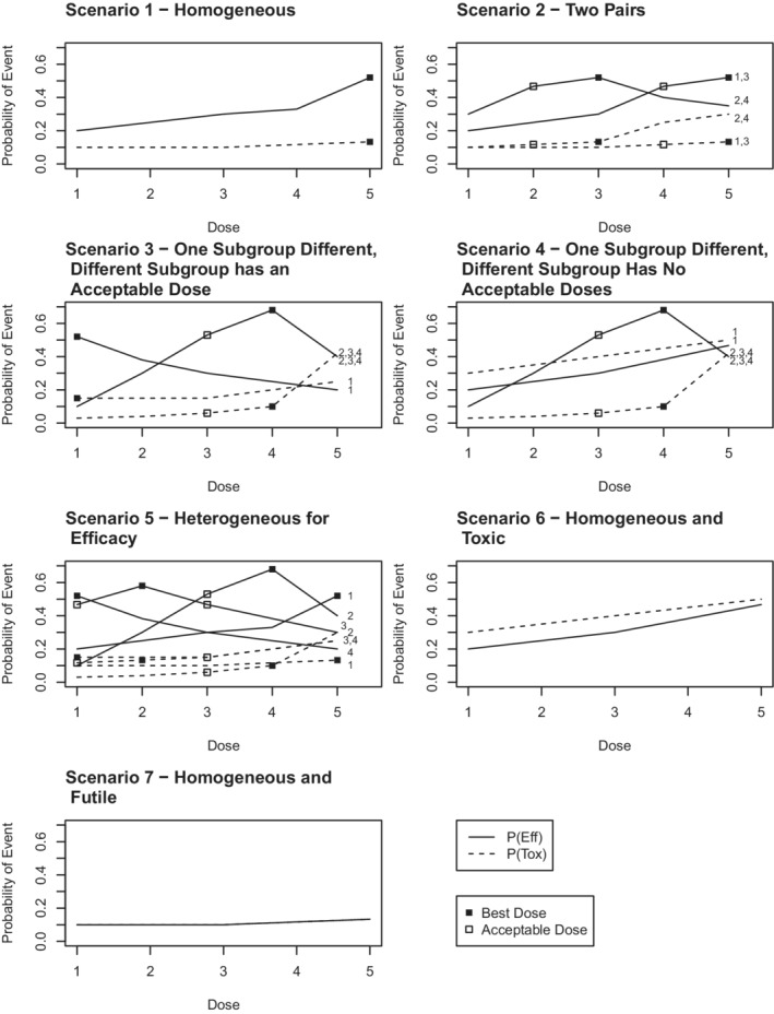
Simulation Scenarios. Each line represents the true probability of efficacy (solid line) or toxicity (dashed line) for some or all of the four subgroups. The number of the subgroup(s) which the line represents (1 through 4) is provided at the right hand side of each plot. In the homogeneous scenarios, the lines provided represent the true probability of efficacy and toxicity for all subgroups. If a square is plotted at a particular dose, it indicates that dose is acceptable for that subgroup. If the square is filled in, that dose is the optimal dose (ie, has the highest utility value) for that subgroup.

All simulation results are based on 1000 trial iterations. In the presented results for Sub‐Eff‐Tox and Sep‐Eff‐Tox models we required convergence of the MCMC samples based on the $97.5$th percentile of a potential scale reduction factor value $\le 1.2$ for each of the subgroup‐specific $\theta$ parameters when fitting the models for each new enrollment. For the hierarchical models, we required convergence based on a multivariate potential scale reduction factor value $\le 1.2$. ²⁷ The simulation study results upon which this study is based are too large to present or store. Therefore, software used to run simulation studies and determine recommended doses using the Sep‐Eff‐Tox and Sub‐Eff‐Tox models have been implemented in Julia ²⁸ and are described in Appendix D in Data S1 and the attached zipped file containing software and a user's guide.

3.3. Simulation results

Here, we averaged subgroup‐specific results over the subgroups. Appendix F in Data S1 contains subgroup‐specific results for the operating characteristics presented in Table 2. Appendix E in Data S1 contains subgroup‐ and dose‐specific true probabilities of efficacy and toxicity, true utility values, true delta values, and the estimated probability of selecting each dose. Additionally, in Appendix I of Data S1 we have provided a couple of example data sets and accompanying utility estimates to illustrate the three estimation approaches (Sep‐Eff‐Tox, hierarchical, and Sub‐Eff‐Tox models) and the estimates a user may obtain from a single data set.

TABLE 2.

Simulation results comparing Sep‐Eff‐Tox, hierarchical, and Sub‐Eff‐Tox methods

	Trial total			Results averaged across subgroups
Subgroup	Estimation method	$P$(Stop)	Duration	$N_{\text{Tox}}$	$N_{\text{Eff}}$	$P{(\text{Sel})}_{\text{Best}}$s	$P{(\text{Sel})}_{\text{Acc}}$	$\mathrm{\Delta }$	$P{(\text{Stop})}_g$	Term	Unterm
Scenario 1‐Homogeneous	Sep‐Eff‐Tox	0.01	4.88	2.52	7.34	0.41	0.41	0.53	0.20	0.79	0.60
	Hierarchical	0.00	4.61	2.66	8.05	0.61	0.61	0.70	0.12	0.57	0.45
	Sub‐Eff‐Tox	0.00	4.65	2.54	7.68	0.58	0.58	0.69	0.12	0.71	0.59
Scenario 2 ‐ Two pairs	Sep‐Eff‐Tox	0.00	4.71	2.91	8.71	0.40	0.59	0.64	0.14	0.55	0.41
	Hierarchical	0.00	4.35	3.07	8.83	0.37	0.60	0.67	0.07	0.32	0.25
	Sub‐Eff‐Tox	0.00	4.40	2.86	8.52	0.35	0.56	0.65	0.04	0.34	0.31
Scenario 3‐ One subgroup different, with acceptable dose	Sep‐Eff‐Tox	0.00	4.37	2.44	11.24	0.60	0.89	0.85	0.05	0.22	0.16
	Hierarchical	0.00	4.31	2.53	11.19	0.58	0.81	0.83	0.03	0.15	0.12
	Sub‐Eff‐Tox	0.00	4.29	2.15	10.61	0.51	0.84	0.84	0.01	0.12	0.11
Scenario 4‐ One subgroup different, no with acceptable dose	Sep‐Eff‐Tox	0.00	4.83	3.01	10.53	0.59	0.91	0.82	0.20	0.57	0.14
	Hierarchical	0.00	4.48	3.62	10.86	0.61	0.96	0.76	0.10	0.33	0.24
	Sub‐Eff‐Tox	0.00	4.59	3.08	10.83	0.58	0.98	0.80	0.12	0.48	0.08
Scenario 5‐ Heterogeneous for efficacy	Sep‐Eff‐Tox	0.00	4.68	2.82	9.84	0.44	0.68	0.68	0.14	0.58	0.44
	Hierarchical	0.00	4.42	2.87	9.43	0.37	0.62	0.66	0.08	0.31	0.23
	Sub‐Eff‐Tox	0.00	4.34	2.62	9.19	0.31	0.59	0.63	0.02	0.21	0.19
Scenario 6‐Homogeneous toxic	Sep‐Eff‐Tox	0.57	5.71	6.95	5.19	0.79	0.00	0.79	0.79	1.75	1.13
	Hierarchical	0.14	6.17	8.30	6.52	0.56	0.00	0.56	0.56	1.80	1.28
	Sub‐Eff‐Tox	0.47	5.94	7.36	5.59	0.72	0.00	0.72	0.72	2.28	1.70
Scenario 7‐ Homogeneous futile	Sep‐Eff‐Tox	0.99	3.94	1.58	1.52	0.99	0.00	0.99	0.99	1.19	0.49
	Hierarchical	0.37	6.63	2.25	2.24	0.77	0.00	0.77	0.77	1.53	0.88
	Sub‐Eff‐Tox	0.97	4.07	1.57	1.50	0.99	0.00	0.99	0.99	1.81	1.11

Abbreviations: $P$(Stop), the probability of terminating the entire trial early. Duration is the mean trial duration (in years) $N_{\text{Tox}}$ and $N_{\text{Eff}}$ are the mean number of patients who experience a toxicity or efficacy event per subgroup; $P{(\text{Sel})}_{\text{Best}}$ and $P{(\text{Sel})}_{\text{Acc}}$, the probability of selecting the best or an acceptable dose for a subgroup, averaged over the subgroups; $\mathrm{\Delta }$, the ${\mathrm{\Delta }}_g$ value for each subgroup, averaged over the subgroups; $P{(Stop)}_g$, the probability of terminating enrollment for a subgroup by the end of the trial, averaged over the subgroups. Term and Unterm are the average number of times enrollment pauses of unpauses during the course of the trial for each subgroup, averaged over the subgroups.

The subgroup simulation results averaged over the subgroups are presented in Table 2. In the homogeneous scenario, we see that Sep‐Eff‐Tox is generally more likely to terminate enrollment than the other methods, especially for the first subgroup which has very conservative priors. Due to the small sample sizes for each separate model, the priors likely play a larger role compared to other models which use all available data. Despite the differences in early enrollment termination, the Sub‐Eff‐Tox method and the hierarchical model are more likely to choose the best or acceptable dose in the homogeneous scenario, which leads to a higher mean $\mathrm{\Delta }$ value, indicating overall better operating characteristics. This is not surprising given that the hierarchical model and Sub‐Eff‐Tox method benefit from borrowing information across subgroups.

The probability of Sub‐Eff‐Tox selecting the best dose for the homogeneous scenarios and scenario 4 is similar to or higher than Sep‐Eff‐Tox, but it is slightly lower for scenarios 2 and 3 and substantially lower for scenario 5. Once again, the probability of enrollment termination plays a role in these differences because although Sep‐Eff‐Tox may have a higher probability of selecting the best dose or an acceptable dose, it also has a higher probability of enrollment termination, which is penalized in the calculation of the ${\mathrm{\Delta }}_g$ term when a subgroup truly has an acceptable dose. The $\mathrm{\Delta }$ values for Sub‐Eff‐Tox are similar to the $\mathrm{\Delta }$ values for Sep‐Eff‐Tox for all scenarios except scenario 1, where the $\mathrm{\Delta }$ values are substantially higher for Sub‐Eff‐Tox. The higher rate of enrollment termination for Sep‐Eff‐Tox is very important to keep in mind when specifying conservative priors, and it may be an advantage to researchers who would like to take a more conservative approach—the mean number of toxicity events is lowest for Sep‐Eff‐Tox in the toxic scenario. However, more frequent enrollment termination carries the disadvantage of prematurely stopping the study of a potentially effective treatment, or the study of a treatment in a subgroup of patients who were likely to benefit. The Sub‐Eff‐Tox method counters this disadvantage of the Sep‐Eff‐Tox method by tuning the prior ${\rho }_{mg}$ values, which provides many of the safety benefits of Sep‐Eff‐Tox with less early termination, and much better handling of homogeneous scenarios.

Relative to Sub‐Eff‐Tox, the hierarchical models have similar $\mathrm{\Delta }$ values for scenarios 1, 2, 3, and 5 as reported in Table 2. However, the hierarchical models have some difficulty choosing the correct dose for scenario 4—where one subgroup needs enrollment terminated, while the other three subgroups should be treated at the same dose. Although the Sub‐Eff‐Tox and hierarchical models have similar $\mathrm{\Delta }$ values in scenario 3—where the first subgroup requires a different dose from the other three—the subgroup‐specific results provided in Appendices E and F in Data S1 show that the probability of selecting the optimal dose for the first subgroup in both scenarios 3 and 4 is much lower for the hierarchical model than the Sub‐Eff‐Tox model (34% vs 48% for scenario 3 and 32% vs 45% for scenario 4 for the hierarchical model and Sub‐Eff‐Tox model, respectively). The poorer performance for the hierarchical models in scenarios 3 and 4 is not surprising considering that hierarchical models assume exchangeability between the subgroups, and that assumption is least appropriate in scenarios 3 and 4. Additionally, the hierarchical models have trouble achieving enrollment termination in the toxic and futile scenarios when it is appropriate to terminate enrollment. We realized that hierarchical models did not escalate doses efficiently unless a lenient prior was used. This sensitivity to prior specification is likely why Cunanan et al ⁵ used a different dose escalation method which encouraged escalation to untested doses if there were no substantial safety (toxicity) concerns.

Additionally, to emphasize the importance of accommodating separate subgroups in the presence of heterogeneity, Appendix J in Data S1 provides simulation results for the seven data generation scenarios presented in Table 2 under the assumption that all patients belong to the same subgroup. Compared to Table 2, the results in Appendix J in Data S1 for scenarios 2 to 5 (ie, scenarios with heterogeneity) have substantially lower $\mathrm{\Delta }$ values.

The number of toxicities per subgroup is generally lowest for Sep‐Eff‐Tox or the Sub‐Eff‐Tox method. The mean number of toxicities per subgroup for the Sep‐Eff‐Tox and Sub‐Eff‐Tox model is within 0.5 toxicity events per subgroup, while the mean number of toxicity events per subgroup is similar for the hierarchical models in most scenarios, but much higher in the toxic and futile scenarios considered. On the other hand, the hierarchical models have a relatively high mean number of efficacy events per subgroup, but only have substantially higher mean number of efficacy events per subgroup for the toxic and futile scenarios, where they did not stop as often as they should. The mean number of efficacy events per subgroup is generally similar for the Sep‐Eff‐Tox and Sub‐Eff‐Tox methods for the scenarios examined, with the possible exceptions of scenarios 3 and 5, where Sep‐Eff‐Tox is slightly higher.

The hierarchical models and Sub‐Eff‐Tox models generally have similar mean trial durations which are shorter than the mean trial durations for Sep‐Eff‐Tox. The futile and toxic scenarios—where Sep‐Eff‐Tox and Sub‐Eff‐Tox models have shorter mean trial durations relative to the hierarchical models—are an exception to this rule. The Sub‐Eff‐Tox model tends to pause and unpause enrollment a relatively low number of times, which is ideal. Exceptions to this trend are noted in scenarios 4, 6, and 7, where enrollment pausing was the ideal choice for at least one subgroup. In practice, frequent pausing and unpausing of enrollment could cause logistical complications and delays.

We also considered two‐subgroup results (presented in Appendix G in Data S1). From these results, we observed that in scenarios with some overlap between acceptable doses for the two groups, the hierarchical and Sub‐Eff‐Tox approaches (the approaches which borrow information across the subgroups) have better performance than the Sep‐Eff‐Tox approach. However, in scenarios where there was no overlap in the optimal doses between the two subgroups, the hierarchical and Sub‐Eff‐Tox models preformed similarly and had slightly lower ${\mathrm{\Delta }}_g$ values compared to Sep‐Eff‐Tox. One slight exception was a scenario where both subgroups had acceptable doses but no overlap in acceptable doses, where the Sub‐Eff‐Tox model preformed slightly worse than the hierarchical model. Overall, if the acceptable doses do not overlap for the two subgroups, the Sep‐Eff‐Tox method has slightly higher ${\mathrm{\Delta }}_g$ values than the two approaches which borrow information across the subgroups.

Researchers who use the Sub‐Eff‐Tox method have the option to modify the prior ${\rho }_{mg}$ values to adjust the prior probability of unclustering. Although we do not present the results here, we have noticed during some limited simulation studies that using a higher prior ${\rho }_{mg}$ values (of 0.9 instead of 0.4) leads to results that more closely resemble Sep‐Eff‐Tox.

As mentioned previously, we have estimated the $\kappa$ parameters from the copula in the Table 2 results. We demonstrate in Appendix H in Data S1 that the results are very similar to those presented in Table 2 of the main manuscript, but note that the efficacy and toxicity outcome data was generated independently and leave further assessment of the benefits of estimating $\kappa$ or assuming independence as an area of further research for the Sub‐Eff‐Tox methodology.

Users of Sub‐Eff‐Tox also need to specify subgroup‐specific prior probabilities for each dose for each subgroup. Although we acknowledge that specifying unique priors for each subgroup can be difficult, we point out that if different subgroups are considered for a trial, this likely indicates some prior beliefs about differences among these patients. To assess the effect of the simplest case, where the same prior probabilities are used for each subgroup, we have run an additional set of simulation studies with the same prior probabilities used for each subgroup (the prior probabilities from subgroup 2 from Table 1). These results are presented in Appendix H in Data S1. In general, the results from using the same prior probability for each subgroup are similar to the results in Table 2, demonstrating that the Sub‐Eff‐Tox methods are reasonably robust to improper prior specification but the operating characteristics tend to benefit slightly from proper prior specification (ie, higher $\mathrm{\Delta }$ values in the homogeneous scenario when the same prior is used for all subgroups, higher $\mathrm{\Delta }$ values for the odd one out scenarios when different priors are used for different subgroups). Users should keep this potential benefit in mind as a motivational factor to use all available information to inform subgroup‐specific priors for Sub‐Eff‐Tox.

Although there are many parameters to calibrate to prepare for a Sub‐Eff‐Tox trial, we believe that it is easier to interpret the effect of changing the prior ${\rho }_{mg}$ values for the Sub‐Eff‐Tox method relative to the hyper variance parameters used to control the amount of borrowing in the hierarchical models. Additionally, these models may benefit from an empirical estimate of the appropriate amount of borrowing part‐way through the trial.

4. CONCLUSIONS

Overall, in the four subgroup scenarios the proposed Sub‐Eff‐Tox method offers the flexibility to handle heterogeneous scenarios as well as Sep‐Eff‐Tox methods, while having substantially better operating characteristics in the presence of homogeneity. The Sub‐Eff‐Tox methods also perform as well as the hierarchical models except when one subgroup has a substantially different optimal dose or when enrollment termination is recommended. In these cases, Sub‐Eff‐Tox methods tend to perform better than the hierarchical models. Depending on the tuning of the ${\rho }_{mg}$ parameters, the Sub‐Eff‐Tox methods may not terminate enrollment as frequently as Sep‐Eff‐Tox methods in unsafe or futile conditions, but the use of the Sub‐Eff‐Tox methods may be preferable if researchers are concerned about dismissing a potentially effective treatment or removing a particular subgroup from consideration in an early trial. Moreover, it is important to consider the role of conservative priors when considering the use of Sep‐Eff‐Tox methods, because prior specifications play a larger role.

This analysis provides plenty of opportunities for future study including the addition of safety features such as a user‐specified run‐in and the option to utilize Sep‐Eff‐Tox methods for a portion of the trial and Sub‐Eff‐Tox methods for another portion of the trial, depending on prior knowledge and/or evidence gathered during the trial. Although we have presented results for these methods in scenarios with two to four subgroups due to what seems practically feasible for an immunologic oncology phase I‐II trial, extension to higher numbers of subgroups is an area of future research. Of note, other authors have explored the effect of different dose‐escalation algorithms in the context of hierarchical models. ⁴ , ⁵ While all models examined in this paper used the same objective function and dose finding algorithm (and any differences between models in these simulation studies are not due to the dose‐escalation algorithm), an area of future study may be to examine more conservative dose‐escalation algorithms on the Sub‐Eff‐Tox methods and whether they improve patient safety. Also, assessing the benefit or detriment of estimating the copula parameter $\kappa$ in the presence of true association between efficacy and toxicity outcomes is another area of further assessment. Furthermore, this modeling framework is adaptable to different distributions of toxicity or efficacy outcomes.

Supporting information

Data S1: Web appendices

Curtis A, Smith B, Chapple AG. Subgroup‐specific dose finding for phase I‐II trials using Bayesian clustering. Statistics in Medicine. 2022;41(16):3164–3179. doi: 10.1002/sim.9410

DATA AVAILABILITY STATEMENT

The simulation study results upon which this study is based are too large to present or store. Therefore, software used to run simulation studies and determine recommended doses using the Sep‐Eff‐Tox and Sub‐Eff‐Tox models have been implemented in Julia and are described in Appendix D in Data S1 and the attached zipped file containing software and a user's guide.

REFERENCES

- 1. Le Tourneau C, Dieras V, Tresca P, Cacheux W, Paoletti X. Current challenges for the early clinical development of anticancer drugs in the era of molecularly targeted agents. Target Oncol. 2010;5:65‐72. [DOI] [PubMed] [Google Scholar]
- 2. O'Quigley J, Paoletti X. Continual reassessment method for ordered groups. Biometrics. 2003;59(2):430‐440. [DOI] [PubMed] [Google Scholar]
- 3. Wages NA, Read PW, Petroni GR. A phase I/II adaptive design for heterogeneous groups with application to a stereotactic body radiation therapy trial. Pharm Stat. 2015;14(4):302‐310. [DOI] [PMC free article] [PubMed] [Google Scholar]
- 4. Cunanan KM, Koopmeiners JS. Hierarchical models for sharing information across populations in phase I dose‐escalation studies. Stat Methods Med Res. 2018;27(11):3447‐3459. [DOI] [PubMed] [Google Scholar]
- 5. Cunanan KM, Koopmeiners JS. Efficacy/toxicity dose‐finding using hierarchical modeling for multiple populations. Contemp Clin Trials. 2018;71:162‐172. [DOI] [PubMed] [Google Scholar]
- 6. Freidlin B, Korn EL. Borrowing information across subgroups in phase II trials: is it useful? Stat Clin Cancer Res. 2013;19(6):1326‐1334. [DOI] [PMC free article] [PubMed] [Google Scholar]
- 7. Cotterill A, Jaki T. Dose‐escalation strategies which use subgroup information. Pharm Stat. 2018;17(5):414‐436. [DOI] [PMC free article] [PubMed] [Google Scholar]
- 8. Salter A, O'Quigley J, Cutter GR, Aban IB. Two‐group time‐to‐event continual reassessment method using likelihood estimation. Contemp Clin Trials 2015;45(Part B):340‐345. [DOI] [PubMed] [Google Scholar]
- 9. Berry DA. A guide to drug discovery: Bayesian clinical trials. Nat Rev Drug Discov. 2006;5(1):27‐36. [DOI] [PubMed] [Google Scholar]
- 10. Thall PF, Wathen JK, Bekele BN, Champlin RE, Baker LH, Benjamin RS. Hierarchical Bayesian approaches to phase II trials in disease with multiple subtypes. Stat Med. 2003;22(5):763‐780. [DOI] [PubMed] [Google Scholar]
- 11. Chugh R, Wathen JK, Maki RG, et al. Phase II multicenter trial of imatinib in 10 histologic subtypes of sarcoma using a Bayesian hierarchical statistical model. J Clin Oncol. 2009;27(19):3148‐3153. [DOI] [PubMed] [Google Scholar]
- 12. Chu Y, Yuan Y. A Bayesian basket trial design using a calibrated Bayesian hierarchical model. Clin Trials. 2018;15(2):149‐158. [DOI] [PMC free article] [PubMed] [Google Scholar]
- 13. Cunanan KM, Iasonos A, Shen R, Gonen M. Variance prior specification for a basket trial design using Bayesian hierarchical modeling. Clin Trials. 2019;16(2):142‐153. [DOI] [PMC free article] [PubMed] [Google Scholar]
- 14. Neuenschwander B, Wandel S, Roychoudhury S, Bailey S. Robust exchangeability designs for early phase clinical trials with multiple strata. Pharm Stat. 2016;15(2):123‐134. [DOI] [PubMed] [Google Scholar]
- 15. Chen N, Lee JJ. Bayesian hierarchical classification and information sharing for clinical trials with subgroups and binary outcomes. Biom J. 2018;61(5):1219‐1231. [DOI] [PMC free article] [PubMed] [Google Scholar]
- 16. Chapple AG, Thall PF. Subgroup‐specific dose finding in phase I clinical trials based on time to toxicity allowing adaptive subgroup combination. Pharm Stat. 2018;17(6):734‐749. [DOI] [PMC free article] [PubMed] [Google Scholar]
- 17. Koopmeiners JS, Modiano J. A Bayesian adaptive phase I‐II clinical trial for evaluating efficacy and toxicity with delayed outcomes. Clin Trials. 2014;11(1):38‐48. [DOI] [PMC free article] [PubMed] [Google Scholar]
- 18. Thall PF, Cook JD. Dose‐finding based on efficacy‐toxicity trade‐offs. Biometrics. 2004;60(3):684‐693. [DOI] [PubMed] [Google Scholar]
- 19. Thall PF, Herrick RC, Nguyen HQ, Venier JJ, Norris JC. Effective sample size for computing prior hyperparameters in Bayesian phase I‐II dose‐finding. Clin Trials. 2014;6(11):657‐666. [DOI] [PMC free article] [PubMed] [Google Scholar]
- 20. Cheung YK, Chappell R. Sequential designs for phase I clinical trials with late‐onset toxicities. Biometrics. 2000;56(4):734‐749. [DOI] [PubMed] [Google Scholar]
- 21. Jin IH, Liu S, Thall PF, Yuan Y. Using data augmentation to facilitate conduct of phase I‐II clinical trials with delayed outcomes. J Am Stat Assoc. 2014;506(109):525‐536. [DOI] [PMC free article] [PubMed] [Google Scholar]
- 22. Murtaugh PA, Fisher LD. Bivariate binary models of efficay and toxicity in dose‐ranging trials. Commun Stat Theory Methods. 1990;19(6):2003‐2020. [Google Scholar]
- 23. Cunanan KM, Koopmeiners JS. Evaluating the performance of copula models in phase I‐II clinical trials under model misspecification. BMC Med Res Methodol. 2014;14(1):1–11. [DOI] [PMC free article] [PubMed] [Google Scholar]
- 24. EffTox. Version 5.2.1. 2021. https://biostatistics.mdanderson.org/SoftwareDownload/SingleSoftware/Index/2;
- 25. Stan Development Team . RStan: the R interface to Stan. R package version 2.19.3. 2020. http://mc‐stan.org/
- 26. R Core Team . R: A Language and Environment for Statistical Computing. Vienna, Austria: R Foundation for Statistical Computing; 2013. [Google Scholar]
- 27. Brooks SP, Gelman A. General methods for monitoring convergence of iterative simulations. J Comput Graph Stat. 1998;7(4):434‐455. [Google Scholar]
- 28. Bezanson J, Edelman A, Karpinski S, Shah VB. Julia: a fresh approach to numerical computing. SIAM Rev. 2017;59(1):65‐98. [Google Scholar]
Associated Data
This section collects any data citations, data availability statements, or supplementary materials included in this article.
Supplementary Materials