Digitized collections elucidate invasion history and patterns of awn polymorphism in Microstegium vimineum

Abstract

Premise

Digitized collections can help illuminate the mechanisms behind the establishment and spread of invasive plants. These databases provide a record of traits in space and time that allows for investigation of abiotic and biotic factors that influence invasive species.

Methods

Over 1100 digitized herbarium records were examined to investigate the invasion history and trait variation of Microstegium vimineum. Presence–absence of awns was investigated to quantify geographic patterns of this polymorphic trait, which serves several functions in grasses, including diaspore burial and dispersal to germination sites. Floret traits were further quantified, and genomic analyses of contemporary samples were conducted to investigate the history of M. vimineum's introduction and spread into North America.

Results

Herbarium records revealed similar patterns of awn polymorphism in native and invaded ranges of M. vimineum, with awned forms predominating at higher latitudes and awnless forms at lower latitudes. Herbarium records and genomic data suggested initial introduction and spread of the awnless form in the southeastern United States, followed by a putative secondary invasion and spread of the awned form from eastern Pennsylvania. Awned forms have longer florets, and floret size varies significantly with latitude. There is evidence of a transition zone with short‐awned specimens at mid‐latitudes. Genomic analyses revealed two distinct clusters corresponding to awnless and awned forms, with evidence of admixture.

Conclusions

Our results demonstrate the power of herbarium data to elucidate the invasion history of a problematic weed in North America and, together with genomic data, reveal a possible key trait in introduction success: presence or absence of an awn.

Invasive species cause billions of dollars in damage to natural, agricultural, and urban systems globally and, together with habitat destruction, represent significant threats to biodiversity, pressures further intensified by globalization and climate change (Simberloff et al., 2013). Yet the causes of invasion success in some species and not others remain an area of intense study (Enders et al., 2018, 2020; Jeschke and Heger, 2018; Dai et al., 2020). While recent introductions provide ideal opportunities to evaluate the mechanisms behind invasion success in situ, established or naturalized invasive species present more of a challenge. Digitized museum collections provide evidence toward a solution, representing powerful tools to broadly study ecology, evolution, systematics, pathology, biogeography, climate change, and invasions (Page et al., 2015; Guralnick et al., 2016; Besnard et al., 2018; McAllister et al., 2018; Borges et al., 2020; Sutherland et al., 2021; Heberling, 2022). Such studies have been facilitated by recent efforts to integrate collections from thousands of institutions into centralized, searchable image databases (e.g., Beaman and Cellinese, 2012; König et al., 2019; Heberling et al., 2021). Consolidated herbarium databases are particularly informative for studies of invasive plant species, allowing an approximation over time and space of introduction history, rate of spread, phenotypic plasticity, and rapid evolution of traits implicated in their invasion success (Crawford and Hoagland, 2009; Marisco et al., 2010; Gallinat et al., 2018). In the absence of direct experimental evidence, digitized specimens allow broad‐scale comparison of similarities or differences in patterns of trait variation among populations between the native and invasive ranges (e.g., morphology, phenology, ecological interactions), as well as the timing of invasion, changes in abundance over time, associations with topography and land use, and overall consequences for biodiversity (e.g., Buswell et al., 2011; Hodgins and Rieseberg, 2011).

Grasses (family Poaceae) are among the most important plants on Earth from economic and ecological perspectives (Linder et al., 2018) and are substantially overrepresented among invasive plant species in both agricultural and natural habitats (Daehler, 1998; Kerns et al., 2020). Invasive grasses pose serious threats to natural, agricultural, and populated areas and have been described as ecosystem engineers capable of altering ecosystem processes including fire regimes, moisture availability, and community dynamics (D'Antonio and Vitousek, 1992; D'Antonio et al., 2017; Fusco et al., 2019; Kerns et al., 2020).

One trait thought to be a key driver of ecological and evolutionary success in grasses is the awn (Humphreys et al., 2011; Linder et al., 2018; McAllister et al., 2019). These bristle‐like extensions of the florets perform a range of functions, for example, in photosynthesis, water stress, dispersal, deterrence of herbivory, and “burial syndrome” (Humphreys et al., 2011; Cavanaugh et al., 2019, 2020; Ntakirutimana and Xie, 2020). “Burial syndrome” relies on a suite of features that assists the diaspore into the soil and increases germination and survival, including a geniculate (bent or twisted) awn morphology (Figure 1A). These geniculate awns demonstrate hygroscopic ability and are sensitive to fluctuations in moisture, changing shape, and moving due to the absorption of water. Increased humidity causes the awn to straighten (Figure 1A–C), and as the awn dries and curls, it drills the diaspore downward, entrapping it in the substrate (Peart, 1979, 1981; Peart and Clifford, 1987; Chambers and MacMahon, 1994; Chambers, 1995; Garnier and Dajoz, 2001). This capability can also propel the diaspores across the surface of the substrate, providing a means of dispersal from dry to moist microsites (Cavanagh et al., 2020).

Figure 1.

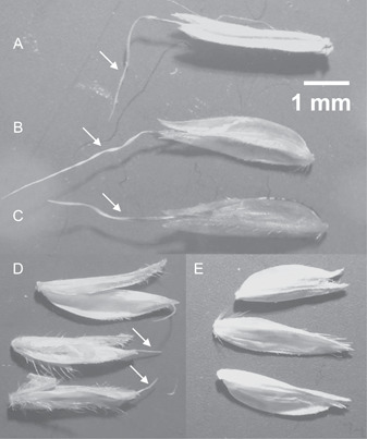
Florets of Microstegium vimineum. (A) Awned floret; arrow indicates the geniculate awn at a 90° angle (fully dried). (B) Awned floret; arrow indicates the geniculate awn at a 45° angle, 1 min after soaking 5 min in water. (C) Awned floret; arrow indicates straightened, geniculate awn immediately after soaking 5 min in water. Florets in A–C are from Tompkins County, New York, USA. (D) Florets with arrows illustrating intermediate, short‐awned phenotypes (Sussex County, Delaware, USA). (E) Awnless florets (Knox County, Tennessee, USA).

Awn morphology has played an important role in grass taxonomy (Hitchcock et al., 1950; Watson and Dallwitz, 1994; Kellogg, 2015). The presence of awned florets is variable across Poaceae and can be polymorphic within species. One such species that displays a presence–absence polymorphism of the awn is Microstegium vimineum (Trin.) A. Camus (stiltgrass; Figure 1), which is native to eastern Asia and highly invasive in eastern North America (Fairbrothers and Gray, 1972; Chen and Phillips, 2007). This annual, C4 grass has become one of the most problematic invaders in eastern North America and is thought to have been introduced as dried packing material in porcelain shipments from Asia (Tu, 2000). It has a mixed mating system, with terminal chasmogamous inflorescences (wind‐pollinated) and axillary, cleistogamous inflorescences (self‐pollinated), allowing production of up to 1000 seeds per plant (Huebner, 2003; Cheplick, 2005). First collected in Knoxville, Tennessee, USA, in 1919, it has spread, over the past century, to 30 U.S. states and southern Canada (Fairbrothers and Gray, 1972; EDDMapS, 2021). Numerous studies have been conducted on the ecological impacts of M. vimineum in the past two decades (e.g., Baker and Dyer, 2011; Flory and Clay, 2010; Huebner, 2010a, 2010b; Rauschert et al., 2010; Barfknecht et al., 2020), yet a comprehensive analysis of its invasion history in eastern North America is lacking. Currently, little is understood about geographic patterns of awn polymorphism in the native and invasive ranges and the eco‐evolutionary implications of its presence or absence.

We examined >1100 digitized herbarium records from Asian and U.S. databases to investigate the invasion history and broad‐scale geographic patterns of awn polymorphism in M. vimineum. Patterns derived from these data represent a crucial, initial step in determining what adaptive significance this trait may have and its potential role in facilitating the establishment and spread of this invasive grass in eastern North America. Further, we included field collections from 31 U.S. populations across the invasive range for genomic analyses, in order to corroborate patterns from digitized records. Our objectives were to investigate the relationships between geography (specifically latitude) and awn polymorphism in M. vimineum to (1) reconstruct the invasion history in the United States, (2) compare broad‐scale geographic patterns of the frequency of awned and awnless forms in Asia vs. the United States, (3) determine if transition zones reveal intermediate awn types, (4) quantify relationships between awn and floret measurements (e.g., awn length, floret length/width, awn bending), (5) compare the abiotic climate conditions that may contribute to the maintenance of awned and awnless forms, and (6) characterize genomic variation and patterns of genetic distinctness among awnless and awned forms in the invasive range.

MATERIALS AND METHODS

Awn data from digitized herbarium sheets

Awn presence–absence data were obtained from several digitized collections databases. For the United States, herbarium records with images were searched via the SouthEast Regional Network of Expertise and Collections (SERNEC, https://sernecportal.org/portal). SERNEC comprises digitized collections from 233 herbaria in 14 U.S. states and further links to several other such consortia. Other searches were conducted using the C.V. Starr Virtual Herbarium (New York Botanical Garden, NY; http://sweetgum.nybg.org), the Smithsonian U.S. National Herbarium (US; https://collections.nmnh.si.edu), and the Ohio State University Herbarium (OS; https://herbarium.osu.edu). Any data that were unavailable in the databases were transcribed from the image of the specimen label. Many specimens without latitude, longitude, or elevation data were georeferenced from the locality information provided, using Google Maps (www.maps.google.com); vague localities that could not be recorded with high confidence (i.e., within 1 km) were excluded. Awn presence–absence was determined by examining the high‐resolution image of each specimen. Non‐flowering specimens, misidentified specimens, and specimens for which awn presence–absence could not be determined with confidence were excluded.

The Chinese Virtual Herbarium (CVH, https://www.cvh.ac.cn), a consortium of over 100 Chinese herbaria containing over five million digitized specimens, was searched for the majority of Asian specimens. Additional digitized specimens were obtained via the Global Biodiversity Information Facility (GBIF, https://www.gbif.org;https://doi.org/10.15468/dl.caar7n), the Herbarium of National Taiwan University (TAI; https://tai2.ntu.edu.tw), the Kagoshima (Japan) University Museum Database (KAG; https://www.museum.kagoshima-u.ac.jp), and the Moscow State University (Russia) Herbarium (MW; https://plant.depo.msu.ru). GPS coordinates and locality information could not be obtained reliably from most Asian records, due to a lack of locality information or language barriers on handwritten specimen labels. Therefore, provincial or regional centroids were used, and awn presence–absence data were summarized as the proportion of specimens with awns present from a particular province/region/state. All Russian records were centered closely around Sochi (Caucasus) and Vladivostok (eastern Siberia), so coordinates for those respective cities were used. Centroids were also recovered for U.S. states, to allow direct comparison of Asian and U.S. specimen data. While centroids obviously provide lower spatial resolution than georeferenced specimen coordinates, they allow for broad‐scale, grouped comparisons of awn presence–absence by region. Centroids were obtained via the R package rworldmap v.1.3.6 (South, 2011).

All subsequent data processing and analyses were conducted in R (R Core Team, 2020). Records were filtered for incomplete data, keeping only unique records (removal of duplicates), using tidyverse v.1.3.1 (Wickham et al., 2019) and dplyr v.1.0.7 (Wickham et al., 2020). Data were then grouped in tidyverse by state (USA, India), province (China), region (Japan), or island (Philippines, Sumatra, Taiwan).

Spatial distribution of awned and awnless records

Base maps for the eastern United States and eastern Asia were generated in rworldmap. The proportion of awned specimens per region and latitude/longitude centroids were specified as a data frame object in R, and pie graphs were placed on maps using the mapPies function in rworldmap. Plots of the proportion of awned specimens vs. latitude were generated with ggplot2 v.3.3.5 (Wickham, 2016). Least‐squares regression of the proportions of awned specimens vs. latitude (i.e., centroid latitude for each region) for Asian and U.S. records was conducted in R. Asian and U.S. specimens were treated separately to allow comparison of patterns between the native and invasive ranges.

Climate variables and awned forms in the United States

In order to address the relationship between the presence–absence of awns and abiotic climate variation in the invasive range, we used publicly available data from WorldClim (https://www.worldclim.org/). The R libraries raster v.3.5.2 and sp v.1.4.5 (Pebesma and Bivand, 2005; Hijmans, 2020) were used to download data for the 19 BIOCLIM variables corresponding to GPS latitude/longitude data for all U.S. specimens at 10 km resolution. In order to mitigate the potentially confounding effects of climate change over the past century, only specimens collected in the year 2000 onward were included, leaving a total of 207 records. The resulting data were subjected to principal component analysis (PCA) in PAST version 4 (Hammer et al., 2001), employing a correlation matrix to account for different scales of the variables. A “broken stick” analysis was applied to the principal components (PCs) to determine the number of PC axes contributing significantly to the total variance in the data set. The PCA was conducted using (1) all BIOCLIM variables (n = 19); (2) temperature‐related variables only (n = 11); and (3) precipitation‐related variables only (n = 8). Nonparametric multivariate analysis of variance (NPMANOVA) was used to test for significant differences in BIOCLIM multivariate space among awned and awnless forms in PAST version 4. PCA loading scores were then exported from PAST and merged with the awn data frame in R. We used logistic regression to test the association between abiotic climate variables and awn presence–absence. Logistic regression was conducted in R among U.S. records, regressing awn presence–absence as a binary response variable on the first principal component for temperature variables, precipitation variables, all BIOCLIM variables, and a model including temperature and precipitation with their interaction term. The model with the lowest Akaike Information Criterion score was used to predict the probability of being awned.

Mapping the invasion history of M. vimineum

Awn data from U.S. specimens were used to create an animated. gif of invasion history using the R packages rgbif v.3.6.0, ggplot2, tidyverse, gganimate v.1.0.7, ggthemes v.4.2.0, sf v.0.9.5, tools v.4.0.2, maps v.3.3.0, rnaturalearth v.0.1.0, and rnaturalearthdata v.0.1.0 (Wickham, 2016; South, 2017; Pebesma, 2018; Chamberlain et al., 2021; Pedersen and Robinson, 2020). The initial, filtered data set was used for the animation, specifying the year collected as an integer to sequentially display the specimen data over time, beginning in 1919 and ending in 2019. An optional feature was added to query GBIF records in the R animation script using rgbif, allowing reconstruction of the invasion history of any organism (based on preserved records, observations, surveys, etc.). The package gganimate was used to produce the final animated figure. We also created a static representation of invasion history at six, roughly 15 yr intervals: 1919–1935, 1936–1950, 1951–1965, 1966–1980, 1981–1995, and 1996–2020. Maps of awned and awnless records were plotted for each time interval with rworldmap, ggplot2, and summarized with ggpubr v.0.4.0 (Kassambra, 2020). Lastly, invasion curves were generated for awnless and awned forms in ggplot2 using the cumulative summary function (cumsum), plotting unique localities over time, with the cumulative number of unique localities binned by year. R code is available at https://rpubs.com/cfb0001/771973.

Floret size, awn length, and intermediate forms

A subset of the U.S. specimens was analyzed more closely to investigate patterns of floret size and awn length variation along a latitudinal “transect” from Mississippi to New York (N = 73 specimens examined). Specifically, forms were sought that displayed intermediate awn morphology between the awnless form and forms with long, exserted, geniculate awns. Only records with GPS coordinates and sufficient image resolution were chosen, to minimize geographical uncertainty as well as error in measurements. Further, specimens were excluded in which multiple plants were present for a specimen and could not be differentiated. Only florets from a single plant were measured per record, with efforts made to measure florets from different inflorescences where possible, choosing the floret from the basal‐most spikelet per raceme. Florets and awns were measured digitally with ImageJ version 2 (Rueden et al., 2017), calibrating the number of pixels to 1.00 cm on the ruler provided for each specimen image. Measurements were taken from five florets per record, selected from racemes distributed along the length of the inflorescence, and only choosing florets that were clearly visible in their entirety. Four features were measured: (1) floret length (i.e., length of the upper lemma, excluding the awn); (2) total floret width at widest point; (3) length of the awn from point of emergence from the floret; and (4) angle of the geniculate awn, from 0–90°, where zero bending = 0° and full bending = 90°. Angle of awn bending was measured using the angle tool in ImageJ, approximated to the nearest 15° increment. All response variables as well as latitude were log₁₀ transformed to mitigate the positive skew in the data. Relationships between latitude, awn type (awnless, short‐awned, and long‐awned; wherein “long‐awned” was determined by awns equal to or greater than the length of the floret) and floret measurements were calculated using a generalized linear mixed model in R in the package lme4 (glmer function; Bates et al., 2015), accounting for non‐independence among the five floret measurements per accession by treating these as a random effect. Tukey‐corrected pairwise comparisons were conducted using the R package multcomp (Hothorn et al., 2008). R code for all analyses is available at https://github.com/barrettlab/Awns-manuscript-R-code/wiki.

Genomic analyses of contemporary U.S. collections

To assess broad‐scale patterns of genetic relationships and population structure in M. vimineum across the invasive range, we sampled 51 individuals (Appendix S1) from 31 localities. We used the CTAB method for DNA extraction (Doyle and Doyle, 1987) from 0.2 g silica‐dried leaf tissue, one individual serving as a voucher from each locality. We used a recently developed protocol based on sequencing of inter‐simple sequence repeat amplicons (ISSR‐seq; Sinn et al., 2021). Briefly, gDNAs were quantified via Qubit Broad Range dsDNA assay (Thermo Fisher Scientific, Waltham, Massachusetts, USA) and diluted to 20 ng/µL for amplification using four ISSR motifs in multiplex from UBC set no. 9 primers 848 [(CA)₈RG], 857 [(AC)₈YG], 868 [(GAA)₆], and 873 [(GACA)₄]. PCR reactions, library preparation, and Illumina NextSeq2000 sequencing (v3 chemistry, 2 × 100 bp paired end reads) were conducted as in Sinn et al. (2021).

Barcoded read sets for each individual were run through a custom pipeline (https://github.com/btsinn/ISSRseq), which comprises a set of UNIX bash scripts to assemble a pseudoreference, clean and map reads to the reference, and call variants following Sinn et al. (2021). The resulting filtered .vcf file was used in downstream analyses. Additionally, ANGSD (Korneliussen et al., 2014) was used to estimate genotype likelihoods from the HaplotypeCaller .bam files produced by GATK (parameters: ‐GL 1 ‐nThreads 20 ‐doGlf 2 ‐doMajorMinor 1 ‐doMaf 2 ‐SNP_pval 2e‐6).

The R package phrynomics was used to further filter the called variants, removing uninformative variants for downstream analysis (https://github.com/bbanbury/phrynomics-data). Relationships among individuals were estimated with SVDQuartets (Chifman and Kubatko, 2014, 2015), under a coalescent model and using all quartets, with 1000 bootstrap replicates to assess branch support. The .vcf file was thinned to a single variant per locus with vcftools (‐thin 3000 option, which is longer than the longest amplicon locus), to account for linkage among sites within loci, and converted to Structure format with PDGSpider (Lischer and Excoffier, 2012). Ancestry coefficients and group membership were estimated using ParallelStructure version 1.0 via the CIPRES Gateway (Miller et al., 2010), with K = 1–5, specifying 200,000 steps and the same number as burn‐in (Besnier and Glover, 2013). Each run was replicated 10 times for each value of K, specifying the admixture model, without specifying population origin as a prior. StructureHarvester (Earl and vonHoldt, 2012) was used to estimate the optimal number of clusters using the “delta K” method (Evanno et al., 2005). Clumpak (http://clumpak.tau.ac.il) was used to summarize results. Lastly, ANGSD version 0.935 was used to output pairwise distances between individuals based on genotype likelihoods (IBS matrix) and subjected to nonmetric multidimensional scaling (NMDS) to identify groupings among the accessions using the R package vegan v.2.4‐2 (metaMDS function; Oksanen et al., 2020).

RESULTS

Awn data from digitized herbarium records

A total of 1145 specimen records remained after filtering records from a total of 2913 available records, with 484 from Asia and 661 from the United States (Appendix S2). In total, 717 were determined to be awnless, while 428 were awned, representing an overall proportion of awned records to be 0.374. The proportion of awned records from Asia was 0.417, while the proportion from the United States was 0.342.

Spatial distribution of awned and awnless proportions

In Asia, both awned and awnless records occur at low and mid‐latitudes (i.e., 0–40°N), while awned records predominate above 40°N latitude (Figure 2). Records from northern China, northern Japan, Siberia, and the Caucasus are predominantly awned, representing the northernmost records in Asia. In the United States (Figure 3), there is a sharp latitudinal transition from predominantly awnless forms in the South (e.g., Alabama, Florida, Georgia, South Carolina, Tennessee) to awned forms in northern states (e.g., Massachusetts, New York, New Jersey, Pennsylvania). At mid‐latitudes—for example, in Maryland, Ohio, Virginia, West Virginia, and North Carolina—there are various proportions of both forms.

Figure 2.

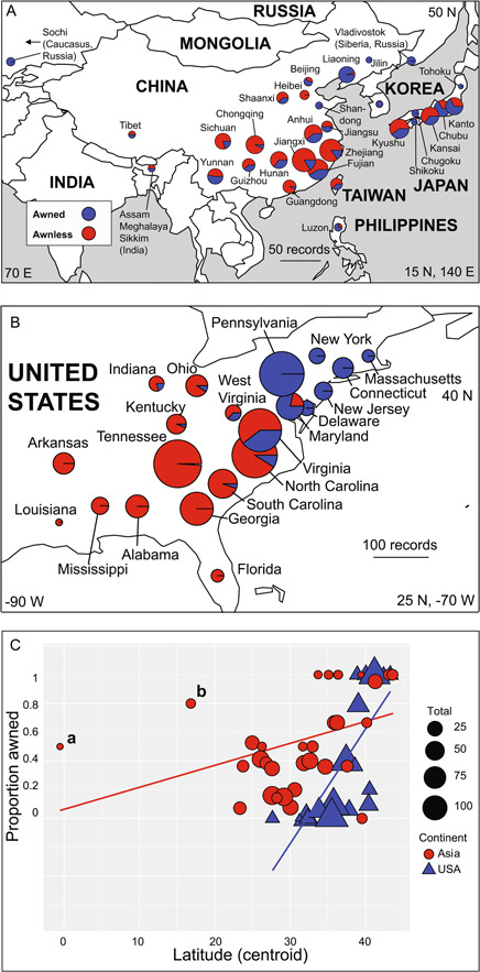
Maps showing the proportions of awned and awnless forms of Microstegium vimineum in (A) Asia (native range) and (B) the United States (introduced range). Pie graphs are scaled proportionally within each map (not between the two maps) to the number of records examined for each centroid. Coordinates given at the corners of each map are degrees latitude and longitude. Arrow in A indicates that Sochi (Caucasus, Russia) is west of the map boundary. (C) Relationship between latitude (degrees north, x‐axis) and the proportion of awned records (y‐axis) for Asian and U.S. records. Total number of records examined for each point is indicated by the scale to the right. Outliers are indicated by ‘a’ (Sumatra) and ‘b’ (Philippines).

Figure 3.

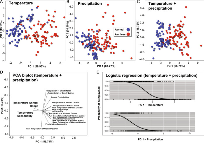
Principal component analysis (PCA) of 19 BIOCLIM variables for all U.S. records of Microstegium vimineum collected after 2000, based on the correlation matrix. Percentages in parentheses on each PC axis represent the total percent variance explained by each axis. (A) BIOCLIM temperature variables. (B) BIOCLIM precipitation variables. (C) All BIOCLIM variables. (D) PCA biplot of temperature and precipitation variables. (E) Logistic regression plots of temperature and precipitation axes (x‐axes) vs. probability of being awned (y‐axes) for U.S. records. Each x‐axis represents the first principal component (PC1) for 11 BIOCLIM temperature variables (above) and eight precipitation variables (below) based on a correlation matrix. Gray shading around logistic regression line indicates 95% confidence interval.

Unweighted regressions revealed a significant, positive relationship between the proportion of awned specimens and latitude in both Asia (Table 1; adjusted R ² = 0.135, p < 0.05) and the United States (Table 1; adjusted R ² = 0.563, p < 0.01). Further regressions of the proportion of awned specimens and latitude—weighted by sample sizes from each centroid—were also significant and positive for U.S. (Table 1; adjusted R ² = 0.673, p < 0.01) and Asian records (Table 1; adjusted R ² = 0.284, p < 0.01). Overall, there was a stronger positive relationship between the proportion of awned records and increasing latitude in the United States, regardless of weighting, compared to Asian records.

Table 1.

Least‐squares regressions of latitude (centroids) vs. the proportion of awned specimens for Asian and U.S. records. Unweighted and weighted regressions (by the total number of records per state, province, or region) are shown.

	Proportion of awned records
	U.S.	U.S. (weighted)	Asian	Asian (weighted)
Latitude coefficient	0.080***	0.105***	0.015**	0.026***
SE	(0.015)	(0.016)	(0.006)	(0.007)
Intercept coefficient	−2.570***	−3.534***	0.063	−0.405*
SE	(0.574)	(0.600)	(0.205)	(0.226)
Observations	21	21	33	33
R 2	0.585	0.689	0.162	0.306
Adjusted R 2	0.563	0.673	0.135	0.284
Residual SE	0.291 (df = 19)	1.322 (df = 19)	0.307 (df = 31)	0.902 (df = 31)
F statistic	26.772*** (df = 1, 19)	42.102*** (df = 1, 19)	5.999** (df = 1, 31)	13.682*** (df = 1, 31)

^* p < 0.1; **p < 0.05; ***p < 0.01

Climate variables and awned forms in the United States

Most BIOCLIM temperature variables had significant, negative correlations with latitude (Appendix S3), while Temperature Annual Range and Temperature Seasonality had significant, positive correlations (Pearson's r = 0.74 and 0.90, respectively; p < 0.001 for both). All precipitation variables were negatively correlated with latitude (p < 0.01 in all cases; Appendix S3). Principal component analysis of 19 BIOCLIM variables (U.S. records only, post‐2000) revealed that the first PC axis explained the majority of overall abiotic climate variation (Figure 3; Appendix S4). This was also the case when analyzing temperature only (PC1 = 66.96%) and precipitation only (PC1 = 63.27%). One‐way, nonparametric multivariate analysis of variance (NPMANOVA) revealed significant differences in multivariate climate space for awned and awnless U.S. records (F = 395.5, p < 0.0001). Logistic regression revealed a negative correlation between both temperature and precipitation and the proportion of awned individuals (p < 0.01 in both cases; Table 2; Figure 3). Of the four models tested (temperature only, precipitation only, all BIOCLIM variables, and temperature × precipitation with interaction), the temperature × precipitation interaction model had the lowest Akaike Information Criterion score (119.953; Table 2). Both temperature and precipitation, and their interaction, were highly significant (p < 0.01). This model correctly classified the probability of being awned vs. awnless in 87.4% of cases.

Table 2.

Logistic regression models for U.S. specimens collected from the year 2000 onward, showing the probability of being awned vs. principal component 1 (PC1) of BIOCLIM temperature and precipitation variables.

	Temp. model	Precip. model	All BIOCLIM model	Temp. × precip. model
Temp. coefficient (PC1)	–1.115***			–1.226***
	–0.147			–0.23
Precip. coefficient (PC1)		–0.965***		–0.760***
		–0.138		–0.253
All BIOCLIM coefficient (PC1)			–1.026***
			–0.14
Temp. (PC1) × precip. (PC1) interaction coefficient				–0.343***
				–0.104
Intercept coefficient	–0.411*	–0.340*	–0.705**	–0.664*
	–0.231	–0.191	–0.274	–0.353
Observations	207	207	207	207
Log likelihood	–65.364	–92.878	–60.237	–55.977
Akaike Information Criterion	134.727	189.757	124.473	119.953

^* p < 0.1; **p < 0.05; ***p < 0.01

Mapping the invasion history of M. vimineum

Animation 1 and Figure 4 show the spread of M. vimineum in the eastern United States, based on digital herbarium records (Animation 1, https://rpubs.com/cfb0001/771973). The first records of the invasion were of the awnless form, which appeared in 1919 (Knox County, Tennessee), followed by a gap in collections until 1931, when it was collected in Harlan County, Kentucky, and Prince George's County, Virginia. By the late 1930s, the awnless form had spread to North Carolina, South Carolina, Georgia, northern Alabama, Kentucky, and southern Ohio. By 1950, it had spread throughout much of Kentucky, Virginia, Ohio, North Carolina, South Carolina, Georgia, and Alabama, while the awned form was restricted to eastern Pennsylvania, New Jersey, and a single record in Virginia. By 1980, the awnless form had spread as far west as Arkansas and Louisiana, while the awned form had spread to Maryland, West Virginia, and North Carolina. The first “awned” records appeared in Berks County, eastern Pennsylvania, in 1938. Interestingly, awned records appeared to have remained concentrated in eastern Pennsylvania and New Jersey from the 1930s until the 1960s, with a few scattered records outside the region during that period. By 1995, the awned form had spread to Connecticut, Massachusetts, eastern New York, and western Pennsylvania. By 2020, it was present throughout much of Pennsylvania and southern New England, and as far west as Indiana. Invasion curve reconstructions (Figure 4G) reveal apparent lag phases for both the awnless and awned forms, followed by linear expansion phases, representing spread from the points of origin. There is no apparent “plateau phase” for either the awned or the awnless form, suggesting continued invasive‐range expansion to date.

Figure 4.

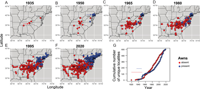
Mapping the invasion history of Microstegium vimineum in the eastern United States. Each slice represents 15 yr (A–F), except for the first (A, 1919–1935) and the last (F, 1995–2020). Red arrow in A = 1919, Knox County, Tennessee (awnless); blue arrow in B = 1938, Berks County, Pennsylvania (awned). (G) Numbers of unique localities colonized over time for awnless and awned forms, binned by year. Dashed line = putative “lag phase” for each.

Floret size, awn length, and intermediate forms

Investigation of 73 U.S. records along a latitudinal gradient from Mississippi to New York revealed the presence of “intermediate,” short‐awned forms, between approximately 37°N and 41°N latitude (Figure 5). Short‐awned records had a mean awn length of 0.169 cm (SD = 0.042 cm, range: 0.10–0.29 cm), whereas longer‐awned records had a mean awn length of 0.464 cm (SD = 0.096, range: 0.27–0.89 cm). Table 3 summarizes the results of generalized linear mixed models comparing floret and awn measurements. Awn lengths were significantly different among short‐awned and long‐awned records (pseudo‐R ² = 0.88, p < 0.001). Notably, these intermediate‐awned records appeared within a latitudinal “transition zone” of overlap between awned and awnless records but were not observed outside of this zone of overlap (Figure 5). The intermediate, short‐awned records further displayed lower values of awn bending (i.e., awn angle) than those with longer awns (Figure 5B; pseudo‐R ² = 0.35, p < 0.001), but this did not vary significantly with latitude when awnless records were removed from the analysis. Floret length (i.e., lemma length, excluding the awn) displayed a positive relationship with latitude (Figure 5C; pseudo‐R ² = 0.65, p < 0.05), whereas floret width did not vary significantly with latitude. The length ratio of awns to florets (considering only awned records) further emphasized the presence of a transition zone between awned and awnless records (Figure 5E). On average, awned records had significantly longer florets than awnless records, excluding the awn itself from measurements (p < 0.001). Specifically, the long‐awned records had significantly longer florets than the short‐awned or awnless records (p < 0.001; Tukey HSD p < 0.05 and p < 0.001, respectively), but short‐awned records did not differ significantly in floret length from awnless records (Tukey HSD, p = 0.494).

Figure 5.

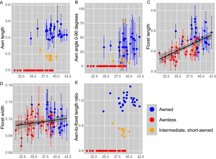
Relationships between awn and floret measurements and latitude for 73 U.S. records of Microstegium vimineum. All measurements are in centimeters except for awn angle and awn:floret length ratio; values are means ± SD, based on five replicate florets per record. Values on x‐axes are °N latitude. (A) Awn length. (B) Degree of awn bending (awn angle). (C) Floret length. (D) Floret width. (E) Awn:floret length ratio.

Table 3.

Mixed‐effects generalized linear regression models for U.S. specimens, showing log₁₀‐transformed awn and floret measurements vs. log₁₀‐latitude and awn type (long, short, or awnless). Fixed‐effect independent variables are shown (left), while random effects were used to account for nonindependent variation in five floret measurements for each accession. Awnless records were removed from the awn angle and awn length regressions to avoid zero values.

	Floret length	Floret width	Awn angle	Awn length
Intercept coefficient	−0.99***	−1.11*	−1.55	0.26
SE	(0.29)	(0.46)	(6.41)	(1.00)
Awn type (long, short, awnless)	−0.05***	−0.03
SE	(0.01)	(0.02)
Awn type (short vs. long)			−0.71***	−0.45***
SE			(0.16)	(0.02)
Log 10 latitude	0.41*	0.12	1.79	−0.37
SE	(0.18)	(0.29)	(4.01)	(0.62)
Pseudo‐ R 2 (fixed effects/total)	0.36/0.65	0.04/0.39	0.19/0.35	0.82/0.88
AIC	−1232.78	−830.19	379.02	−360.32
BIC	−1209.46	−806.87	395.12	−344.22
Log likelihood	622.39	421.09	−184.51	185.16
Number of observations	360	360	185	185
Number of groups: accession	72	72	37	37
Variance: accession (intercept)	0.00	0.00	0.09	0.00
Variance: residual	0.00	0.00	0.37	0.01

^* p < 0.1; **p < 0.05; ***p < 0.01

Genomic relationships and population structure in the invasive range

Sequencing of ISSR amplicons yielded 4714 final, called variants after conservative processing and filtering with GATK for 51 accessions from 31 localities (Appendix S5). After filtering non‐parsimony‐informative variants, 1565 variants remained for phylogenetic analysis. Phylogenetic analysis in SVDQuartets under a coalescent model showed overall strong support (all branches had bootstrap values of 100), with two clearly defined clades corresponding to awned and awnless forms (Figure 6A). One awnless accession from western North Carolina, USA (NC SP 2‐6) grouped closely with awned accessions from Ohio and New York, USA, but otherwise all awned and awnless accessions grouped together correspondingly. The NMDS plot (Figure 6B) based on a distance matrix from genotype likelihoods for 39,198 variants yielded a similar overall pattern to the phylogenetic analysis, with awned and awnless accessions separated along NMDS axis 1; again, the exception was accession NC SP 2‐6 from North Carolina. Structure analysis (Figure 6C) further supported these findings, with K = 2 as the optimal number of genomic clusters based on the “delta K” method and the current sampling of accessions (K = 477.7; Appendix S6). Awned and awnless forms generally comprised distinct clusters, though there was some evidence for admixture, with the awnless NC SP 2‐6 being a notable outlier. Specifically, there is limited evidence of admixture among the more northern, awned accessions, and the more southern, awnless accessions. A few awnless accessions from Kentucky, Illinois, Ohio, Virginia, and Tennessee showed some evidence of mixed ancestry among the two clusters, while some awned accessions from Pennsylvania, Virginia, New York, Ohio, Maryland, and West Virginia displayed similar patterns of mixed ancestry.

Figure 6.

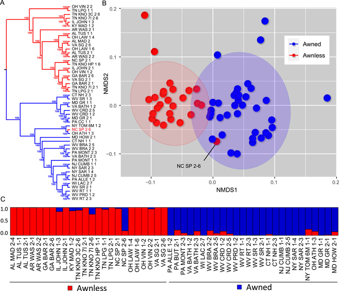
Genomic analyses of field‐collected U.S. Microstegium vimineum accessions. (A) Coalescent‐based phylogenetic analysis of 1565 SNPs with SVDQuartets, with parsimony‐uninformative SNPs removed. Numbers adjacent to branches indicate bootstrap support values (1000 pseudoreplicates). Red=awnless, blue=awned. (B) Nonmetric multidimensional scaling ordination plot based on a pairwise distance matrix from ANGSD genotype likelihoods of 39,198 SNPs (K = 3 dimensions, stress = 0.176). (C) Ancestry plot based on 3148 SNPs after linkage disequilibrium thinning in ParallelStructure (highest ΔK was 477.7 for K = 2).

DISCUSSION

By analyzing >1100 digital herbarium records of the invasive M. vimineum, we were able to reconstruct the invasion history of this species in the United States, detect evidence of at least two putative invasions, demonstrate strikingly similar geographic patterns of awn presence–absence polymorphism in the native and invasive ranges, and characterize patterns of floret and awn variation along a latitudinal gradient. The inclusion of genomic data from 51 contemporary samples demonstrates the distinctness of awned and awnless forms, with some evidence of admixture, and supports the hypothesis of multiple introductions to the United States. This study represents the most comprehensive use of digitized collections data for M. vimineum to date, underscoring the importance of herbaria and of efforts to centralize digitized collections globally to begin to elucidate a plant's invasive success.

The potential role of awns in invasiveness of M. vimineum

Our data show a unique pattern of awn polymorphism, contributing to a novel hypothesis for its adaptive role in burial at higher latitudes. Würschum et al. (2020) found evidence of long and intermediate awn lengths in wheat at lower latitudes, and Li et al. (2015) found that awn mass was negatively correlated with latitude, the opposite of our findings in M. vimineum, which they explain as either an adaptation to drier conditions or as having been artificially selected by growers. Grundbacher (1963) suggested that awns in more moist habitats may provide additional surface area for infection by soilborne pathogens, thus potentially explaining the lack of awns at lower latitudes where precipitation is higher (Figure 2). In the native grass Sorghastrum nutans (L.) Nash, shorter awns were observed in the southeastern United States, while intermediate or longer awns were observed elsewhere, but the explanation for this pattern is unclear (Soper Gorden et al., 2016). There has been a significant amount of research on the adaptive value of awns in fire‐prone regions (e.g., in African, Australian, and South American grasslands) with respect to increased survival and burial depth (e.g., Garnier and Dajoz, 2001; Johnson and Baruch, 2014). Individual diaspores with longer, hygroscopic awns typically have superior ability to find safe sites and to bury deeper in the soil, especially those with geniculate (twisted or bent) awns, thereby decreasing seed mortality (Cavanagh et al., 2020), though the type of substrate is also important (smaller soil particle size results in greater burial depth; Molano‐Flores, 2012).

What, then, could explain the prevalence of awned forms in M. vimineum at higher latitudes in Asia and the United States (Figure 2)? Fire does not appear to be a logical explanation for the prevalence of awns in this species, given that large fires are less frequent in the eastern United States than in drier regions in the western United States, and actually have a higher incidence in the Southeast (where awnless forms predominate) than in the Northeast and Upper Midwest (e.g., Rudis and Skinner, 1991; Munn et al., 2003; Ryan and Opperman, 2013). Precipitation differences between the Northeast and Southeast might explain this pattern, but these differences in precipitation are not extreme (i.e., the latitudinal pattern in precipitation is weaker than that for temperature; Appendix S3); moreover, precipitation is heterogeneous throughout the eastern United States as a result of longitude, elevation, and other factors (Peel et al., 2007).

One plausible hypothesis is that soil freezing explains the north–south pattern in awn presence–absence, putatively providing a mechanism for habitat filtering post‐introduction (sensu Weiher and Keddy, 1995). Though support in the literature for this geographic pattern is limited, there is evidence of awns being used for seed burial in alpine systems, and a greater likelihood of seeds with awns being found in alpine seedbanks (Chambers, 1995). In addition, buried seed of the awned grass Bromus setifolius var. pictus (Hook. f.) Skottsb. in a Patagonian steppe (temperatures average around 3°C) had greater survival as seedlings than unburied seed (Rotundo and Aguiar, 2004). Plants have evolved various mechanisms to survive freezing temperatures at higher latitudes and altitudes (Ambroise et al., 2020). Reliance on mechanisms such as underground perennating organs is not applicable for M. vimineum, which, as an annual grass, relies completely on recruitment from the seed bank (Gibson et al., 2002; Redwood et al., 2018). Thus, to survive the more intense freezing cycles experienced at higher latitudes, seeds or seed dispersal units must be adapted to survive extreme conditions.

Alternatively, alleles associated with awn formation may be linked to others that could better explain the north–south latitude pattern. For instance, silica deposition genes or their expression have been associated with awn development or expression (Peleg et al., 2010; Yamaji et al., 2012; Ntakirutimana and Xie, 2019). Silica in plants is important for structural support and defense against fungal pathogens and herbivory (Currie and Perry, 2007). Silica also slows plant tissue decomposition in some grasses (Miyake and Takahashi, 1983; Schaller et al., 2014). Theoretically, buried seed, especially over long periods, may need more protection from fungal pathogens, whereas some populations with extended growing seasons and large individuals may benefit more from increases in available nutrients in response to rapid decomposition. Plants with more silica and awns may further lead to formation of a longer‐term seed bank, whereas lack of silica and awns may equate to a shorter‐term seed bank and subsequent differences in seed longevity and/or dormancy.

To our knowledge, the geographic pattern of awn polymorphism in M. vimineum is the only case where such a north–south, awned–awnless pattern has been documented in grasses (e.g., Soper Gorden et al., 2016). Similar investigations of awns in other grass species spanning subtropical to temperate ranges, including invasive grasses, should be conducted to establish corroborating evidence for this pattern. Awns serve a variety of functions in grasses, and these roles are highly context‐dependent (e.g., Humphreys et al., 2011; Schrager‐Lavelle et al., 2017). Therefore, if awns are indeed adaptive for soil burial at higher latitudes, this would represent a novel ecological context for the function of this trait and its role in invasion success. The fact that intermediate, short‐awned forms were observed at relative low frequency at mid‐latitudes suggests that awned and awnless forms intergrade where their ranges overlap (Figure 5), that this trait is likely under genetic control, and that there may be selection against intermediate forms at both higher and lower latitudes (i.e., reinforcement; Dobzhansky, 1940; Harrison, 1993; Coyne and Orr, 1998; Curry, 2015). Clearly, additional study is needed to quantify the contribution of awns or other (possibly linked) traits to invasion success in this species.

Invasion history of M. vimineum via herbarium records

Our analysis of digitized herbarium records in the eastern United States provides historical evidence of at least two separate invasions by M. vimineum. The initial invasion likely happened somewhere in the southeastern United States (based on the initial 1919 Tennessee collection and subsequent collections in Tennessee, Kentucky, Virginia, North Carolina, and northern Alabama; Figure 4). It is impossible to determine exactly when or where this initial introduction occurred, and it could have occurred much earlier than 1919, perhaps in the late 1800s. A secondary invasion in the 1930s in eastern Pennsylvania is evident, with only localized initial spread there and in neighboring New Jersey (Figure 4). The gap between the initial collection by Ainslie (1919, Knox County, Tennessee) and both of the 1931 collections by Braun and Blake (Harlan County, Kentucky, and Prince George County, Virginia, respectively) may be the result of low initial, post‐introduction abundance, lack of familiarity with M. vimineum by collectors at that time, or separate, additional introductions (Fairbrothers and Gray, 1972).

The second putative introduction (i.e., awned form) and, to a lesser degree, the first introduction (awnless form) display characteristic lag phases, in which they appear to establish locally or regionally prior to a more rapid expansion (Figure 4A,B,G; Hengveld, 1988, 1989; Hobbs and Humphreys, 1995). The lag phase can have different causes, related to demography, changing environmental conditions, or genetic potential (Crooks and Soulé, 1999). While it is impossible to discern what the causes of the lag phase would have been for each of these putative introductions, investigation of genomic variation from herbarium samples, in combination with data on past environments and the temporal dynamics of anthropogenic disturbance over the past century, may shed light on this observation.

Genomic analysis of 51 accessions from contemporary field collections across the eastern United States displays a strong pattern of differentiation among awnless and awned forms (Figure 6). This finding provides further evidence for at least two separate invasions by M. vimineum in the United States. There is also limited evidence of admixture between the two forms in some accessions, most notably in one awnless accession from Mitchell County in northwestern North Carolina (NC SP 2‐6), but also in several others. Novy et al. (2013) provided evidence of clinal variation in phenology and vegetative biomass at anthesis with latitude, their main conclusion being that this invasive species has rapidly adapted within the introduced range over the past century. Given the annual life history of M. vimineum, this provides >100 generations over which evolution could have occurred. As an alternative explanation for this pattern, Novy et al. (2013) stated: “IBD [isolation by distance] could result from the northern phenotype (i.e., shorter time to flowering at lower biomass) being introduced in the northern United States and the southern phenotype (i.e., longer time to flowering at higher biomass) being introduced in the southern United States.” Although rapid evolution in flowering time over a century could have resulted from a single introduction of an invasive annual plant (given that there was sufficient genetic variation present), our findings suggest that the alternative scenario posited by Novy et al. (2013) is equally plausible, and possibly not mutually exclusive of their primary explanation of this pattern.

A regional genetic study of populations in northern and eastern West Virginia, USA (Culley et al., 2016), suggested that while a significant amount of population structure exists for M. vimineum, there is also evidence for long‐ or at least intermediate‐distance dispersal, likely mediated by human activity or movement via water (Huebner, 2007, 2010b; Christen and Matlack, 2009; Tekiela and Barney, 2013). The persistence of two distinct forms in the United States—awnless in the Southeast and awned in the North—suggests the possibility that both invasion history and selection for awned/awnless forms at higher/lower latitudes may have played roles in the current distribution and expansion of this species, though experimental evidence is needed to determine whether selection via habitat filtering (i.e., preadapted invasion) has played a role. The rationale here is that even if, for example, long‐distance seed dispersal is common in the invasive range, selection could counteract the predominantly homogenizing effects of gene flow, reinforcing the existence of awned forms at high latitudes and awnless forms at low latitudes, removing maladaptive alleles introduced by seed dispersal, but maintaining new genotypic combinations that allow local adaptation (e.g., Edelaar and Bolnick, 2012).

Admixture is now well known as a potential source of adaptive variation among multiple source introductions of invasive species (Dlugosch and Parker, 2007; Keller and Taylor, 2010; Keller et al., 2014; van Boheemen et al., 2017, 2018; Lachmuth et al., 2019), and has possibly played a role in local adaptation and continued range expansion of M. vimineum in North America. Following the rationale of Novy et al. (2013), if two successful invasions have indeed occurred (southern awnless and northern awned, respectively), then subsequent admixture and allelic shuffling could potentially allow the expression of novel phenotypes associated with phenology, physiology, and morphology, allowing “fine tuning” of localized adaptation. Thus, if introductions of M. vimineum were frequent enough over time, then the invasion success of this species could at least partially be explained by a combination of habitat filtering and propagule pressure (Weiher and Keddy, 1995; Lockwood et al., 2005). In other words, there may have been many opportunities to “get it right” in terms of each initial invasion being preadapted to some degree—especially if low genetic diversity was associated with introduction bottlenecks—and subsequent spread, admixture, and selection all may have contributed to invasion success.

CONCLUSIONS

We present the first comprehensive analysis of invasion history and intraspecific awn polymorphism in M. vimineum, relying on >1100 digitized herbarium records from centralized databases. We demonstrate historical and contemporary‐genomic evidence of at least two separate invasions in the United States, a scenario that is increasingly becoming apparent in invasion biology (e.g., Keller and Taylor, 2010; Sutherland et al., 2021; Vallejo‐Marín et al., 2021). A combination of habitat filtering, M. vimineum being an “ideal weed” (in reference to awn traits), propagule pressure (i.e., the possibility of several introductions), and other factors may explain the success of this invasive species and represent plausible hypotheses for future investigation. Alhough M. vimineum has several plastic traits, these data support multiple introductions of the two awn forms and possible subsequent habitat filtering instead of plasticity of the awn trait.

While we hypothesize that habitat filtering may explain the success of the awned form in colder climates, more research is needed to explain the potential adaptive advantage of being awnless in warmer climates. Additional genomic analyses of material from herbarium specimens across space and time will allow more nuanced reconstruction of invasion history and determination of invasion mechanisms, providing further insights into any adaptive processes at the genomic level—that is, by evaluating the relatedness of co‐occurring awn types and estimating how long it takes awnless and awned forms to become extant in colder and warmer climates, respectively, thereby determining a rate of habitat filtering or competitive ability between the two forms. Our results further highlight the need for experimental studies, specifically exploring the role of awns and other potential trait polymorphisms in invasiveness. For example, seed bank germination studies or burial experiments using awned, awnless, and intermediate awned forms under different soil temperature/moisture regimes could be informative on fitness metrics such as germination rates, seed bank accumulation and viability over time, the effect of burial depth, differences in dormancy, and seedling survival to reproductive stage (e.g., Ramos et al., 2019). These data could also be used to better incorporate site invasibility with plant invasiveness by correlating local landscapes and physiography with invasion history, perhaps highlighting patterns along rivers and other corridors. Ultimately, what we have learned from the use of historical records of M. vimimeum can be applied to other established plant invaders and may help us predict and prevent future invasions.

AUTHOR CONTRIBUTIONS

C.F.B. and C.D.H. conceived of the study. C.F.B. conducted all data analyses and wrote the manuscript. C.D.H., Z.A.B., T.A.B., M.V.S., C.W.C., H.L.T., S.V.S., and A.N.C. compiled data and helped write the manuscript. M.L., M.R.M., and M.M. provided helpful discussion and helped write the manuscript. All authors contributed critically to the drafts and gave final approval for publication.

CONFLICT OF INTEREST

There are no conflicts of interest to report.

Supporting information

Appendix S1. Sampling localities for contemporary genomic samples of Microstegium vimineum.

Appendix S2. Summary of 1145 digitized specimen records of Microstegium vimineum.

Appendix S3. Spearman's correlation coefficients and significance for latitude (°N) vs. each of the 19 BIOCLIM variables for all U.S., post‐2000 records for Microstegium vimineum.

Appendix S4. Principal component loadings of 19 BIOCLIM variables.

Appendix S5. Voucher, locality, and collector information for contemporary field samples of Microstegium vimineum used in genomic analyses.

Appendix S6. Evaluation of the most likely number of ancestral populations/genetic clusters from the ParallelStructure analyses.

Barrett, C. F. , Huebner C. D., Bender Z. A., Budinsky T. A., Corbett C. W., Latvis M., McKain M. R., Motley M., Skibicki S. V., Thixton H. L., Santee M. V., and Cumberledge A. N.. 2022. Digitized collections elucidate invasion history and patterns of awn polymorphism in Microstegium vimineum . American Journal of Botany 109(5): 689–705. 10.1002/ajb2.1852

DATA AVAILABILITY STATEMENT

Data extracted from herbarium image databases and genomic.vcf files (filtered and linkage disequilibrium‐thinned variants) are provided at https://doi.org/10.5281/zenodo.6384405. Raw genomic data are provided in the Sequence Read Archive as FASTQ files (https://www.ncbi.nlm.nih.gov/sra) under BioProject PRJNA773774. R code used for this paper can be found at https://rpubs.com/cfb0001 and https://github.com/barrettlab/Awns-manuscript-R-code/wiki.

REFERENCES

- Ambroise, V. , Legay S., Guerriero G., Hausman J.‐F., Cuypers A., and Sergeant K.. 2020. The roots of plant frost hardiness and tolerance. Plant and Cell Physiology 61: 3–20. [DOI] [PMC free article] [PubMed] [Google Scholar]
- Barfknecht, D. F. , Gibson D. J., and Neubig K. M.. 2020. Plant community and phylogenetic shifts in acid seep springs over 49 years following Microstegium vimineum invasion. Plant Ecology 221: 167–175. [Google Scholar]
- Baker, S. A. , and Dyer R. J.. 2011. Invasion genetics of Microstegium vimineum (Poaceae) withinthe James River Basin of Virginia, USA. Conservation Genetics 12: 793–803. [Google Scholar]
- Bates, D. , Mächler M., Bolker B., and Walker S.. 2015. Fitting linear mixed‐effects models using lme4. Journal of Statistical Software 67: 1–48. [Google Scholar]
- Beaman R. S., and Cellinese N.. 2012. Mass digitization of scientific collections: New opportunities to transform the use of biological specimens and underwrite biodiversity science. Zookeys 209: 7–17. [DOI] [PMC free article] [PubMed] [Google Scholar]
- Besnard, G. , Gaudeul M., Lavergne S., Muller S., Rouhan G., Sukhorukov A. P., Vanderpoorten A., and Jabbour F.. 2018. Herbarium‐based science in the twenty‐first century. Botany Letters 165: 323–327. [Google Scholar]
- Besnier F., and Glover K. A.. 2013. ParallelStructure: A R package to distribute parallel runs of the population genetics program STRUCTURE on multi‐core computers. PLoS One 8: e70651. [DOI] [PMC free article] [PubMed] [Google Scholar]
- Borges, L. M. , Reis V. C., and Izbicki R.. 2020. Schrödinger's phenotypes: Herbarium specimens show two‐dimensional images are both good and (not so) bad sources of morphological data. Methods in Ecology and Evolution 11: 1296–1308. [Google Scholar]
- Buswell, J. M. , Moles A. T., and Hartley S.. 2011. Is rapid evolution common in introduced plant species? Journal of Ecology 99: 214–224. [Google Scholar]
- Cavanagh, A. M. , Godfree R. C., and Morgan J. W.. 2019. An awn typology for Australian native grasses (Poaceae). Australian Journal of Botany 67: 309–334. [Google Scholar]
- Cavanagh, A. M. , Morgan J. W., and Godfree R. C.. 2020. Awn morphology influences dispersal, microsite selection and burial of Australian native grass diaspores. Frontiers in Ecology and Evolution 8: 389. [Google Scholar]
- Chambers, J. C. 1995. Relationships between seed fates and seedling establishment in an alpine ecosystem. Ecology 76: 2124–2133. [Google Scholar]
- Chambers, J. C. , and MacMahon J. A.. 1994. A day in the life of a seed: Movements and fates of seeds and their implications for natural and managed systems. Annual Review of Ecology and Systematics 25: 263–292. [Google Scholar]
- Chen, S. , and Phillips S. M.. 2007. Microstegiumvimineum. In: Wu Z. Y., Raven P. H., and Hong D. Y. (Eds.), Flora of China 175–180. Science Press, Beijing, China: and Missouri Botanical GardenPress. [Google Scholar]
- Cheplick, G. P. 2005. Biomass partitioning and reproductive allocation in the invasive, cleistogamous grass Microstegium vimineum: Influence of the light environment. The Journal of the Torrey Botanical Society 132: 214–224. [Google Scholar]
- Chifman, J. , and Kubatko L.. 2014. Quartet inference from SNP data under the coalescent. Bioinformatics 30: 3317–3324. [DOI] [PMC free article] [PubMed] [Google Scholar]
- Chifman, J. , and Kubatko L.. 2015. Identifiability of the unrooted species tree topology under the coalescent model with time‐reversible substitution processes, site‐specific rate variation, and invariable sites. Journal of Theoretical Biology 374: 35–47. [DOI] [PubMed] [Google Scholar]
- Christen, D. C. , and Matlack G. R.. 2009. The habitat and conduit functions of roads in the spread of three invasive plant species. Biological Invasions 11: 453–465. [Google Scholar]
- Coyne, J. A. , and Orr H. A.. 1998. The evolutionary genetics of speciation. Philosophical Transactions of the Royal Society of London. Series B: Biological Sciences 353: 287–305. [DOI] [PMC free article] [PubMed] [Google Scholar]
- Crawford, P. H. C. , and Hoagland B. W.. 2009. Can herbarium records be used to map alien species invasion and native species expansion over the past 100 years? Journal of Biogeography 36: 651–661. [Google Scholar]
- Crooks, J. A. , and Soulé M. E.. 1999. Lag times in population explosions of invasive species: Causes and implications. In: Sandlund O., Schei P., and Viken A. (Eds.), Invasive species and biodiversity management. 103–125. Kluwer Academic Press. [Google Scholar]
- Culley, T. M. , Huebner C. D., and Novy A.. 2016. Regional and local genetic variation in Japanese stiltgrass (Microstegium vimineum). Invasive Plant Science and Management 9: 96–111. [Google Scholar]
- Currie, H. A. , and Perry C. C.. 2007. Silica in plants: biological, biochemical and chemical studies. Annals of Botany 100: 1383–1389. [DOI] [PMC free article] [PubMed] [Google Scholar]
- Curry, C. M. 2015. An integrated framework for hybrid zone models. Evolutionary Biology 42: 359–365. [Google Scholar]
- D'Antonio, C. M. , and Vitousek P. M.. 1992. Biological invasions by exotic grasses, the grass/fire cycle, and global change. Annual Review of Ecology and Systematics 23: 63–87. [Google Scholar]
- D'Antonio, C. M. , Yelenik S. G., and Mack M. C.. 2017. Ecosystem vs. community recovery 25 years after grass invasions and fire in a subtropical woodland. Journal of Ecology 105: 1462–1474. [Google Scholar]
- Daehler, C. C. 1998. The taxonomic distribution of invasive angiosperm plants: Ecological insights and comparison to agricultural weeds. Biological Conservation 84: 167–180. [Google Scholar]
- Dobzhansky, T. 1940. Speciation as a stage in evolutionary divergence. The American Naturalist 74: 312–321. [Google Scholar]
- Doyle, J. J. , and Doyle J. L.. 1987. A rapid DNA isolation procedure for small quantities of fresh leaf tissue. Phytochemical Bulletin 19: 11–15. [Google Scholar]
- Earl, D. A. , and vonHoldt B. M.. 2012. STRUCTURE HARVESTER: a website and program for visualizing STRUCTURE output and implementing the Evanno method. Conservation Genetics Resources 4: 359–361. [Google Scholar]
- EDDMapS . 2021. Early Detection & Distribution Mapping System. Website https://www.eddmaps.org/
- Edelaar, P. , and Bolnick D. I.. 2012. Non‐random gene flow: An underappreciated force in evolution and ecology. Trends in Ecology and Evolution 27: 659–665. [DOI] [PubMed] [Google Scholar]
- Enders, M. , Havemann F., Ruland F., Bernard‐Verdier M., Catford J. A., Gómez‐Aparicio L., Haider S., et al. 2020. A conceptual map of invasion biology: Integrating hypotheses into a consensus network. Global Ecology and Biogeography 29: 978–991. [DOI] [PMC free article] [PubMed] [Google Scholar]
- Enders, M. , Hütt M.‐T., and Jeschke J. M.. 2018. Drawing a map of invasion biology based on a network of hypotheses. Ecosphere 9: e02146. [Google Scholar]
- Evanno, G. , Regnaut S., and Goudet J.. 2005. Detecting the number of clusters of individuals using the software structure: a simulation study. Molecular Ecology 14: 2611–2620. [DOI] [PubMed] [Google Scholar]
- Fairbrothers, D. E. , and Gray J. R.. 1972. Microstegium vimineum (Trin.) A. Camus (Gramineae) in the United States. Bulletin of the Torrey Botanical Club 99: 97. [Google Scholar]
- Flory, S. L. , and Clay K.. 2010. Non‐native grass invasion suppresses forest succession. Oecologia 164: 1029–1038. [DOI] [PubMed] [Google Scholar]
- Fusco, E. J. , Finn J. T., Balch J. K., Nagy R. C., and Bradley B. A.. 2019. Invasive grasses increase fire occurrence and frequency across US ecoregions. Proceedings of the National Academy of Sciences of the United States of America 116: 23594–23599. [DOI] [PMC free article] [PubMed] [Google Scholar]
- Gallinat, A. S. , Russo L., Melaas E. K., Willis C. G., and Primack R. B.. 2018. Herbarium specimens show patterns of fruiting phenology in native and invasive plant species across New England. American Journal of Botany 105: 31–41. [DOI] [PubMed] [Google Scholar]
- Garnier, L. K. M. , and Dajoz I.. 2001. Evolutionary significance of awn length variation in a clonal grass of fire‐prone savannas. Ecology 82: 1720–1733. [Google Scholar]
- Gibson, D. J. , Spyreas G., and Benedict J.. 2002. Life history of Microstegium vimineum (Poaceae), an invasive grass in southern Illinois. Journal of the Torrey Botanical Society 129: 207. [Google Scholar]
- Grundbacher, F. 1963. The physiological function of the cereal awn. The Botanical Review 29: 366–381. [Google Scholar]
- Guralnick, R. P. , Zermoglio P. F., Wieczorek J., LaFrance R., Bloom D., and Russell L.. 2016. The importance of digitized biocollections as a source of trait data and a new VertNet resource. Database 2016: baw 1 58. [DOI] [PMC free article] [PubMed] [Google Scholar]
- Hammer, Ø. , Harper D. A. T., and Ryan P. D.. 2001. PAST: Paleontological statistics software package for education and data analysis. Palaeontologia Electronica 4: 9. [Google Scholar]
- Harrison, R. G. 1993. Hybrid zones and the Evolutionary Process. 364 pp. Oxford University Press, Oxford, U.K.
- Heberling, J. M. 2022. Herbaria as big data sources of plant traits. International Journal of Plant Sciences 183: 87–118. [Google Scholar]
- Heberling, J. M. , Miller J. T., Noesgaard D., Weingart S. B., and Schigel D.. 2021. Data integration enables global biodiversity synthesis. Proceedings of the National Academy of Sciences 118: e2018093118. [DOI] [PMC free article] [PubMed] [Google Scholar]
- Hijmans, R. J. 2020. raster: Geographic data analysis and modeling. R package version 3.0‐12. Website: https://CRAN.R-project.org/package=raster
- Hitchcock, A. S. , Chase A., and United States . (1950). Manual of the grasses of the United States: Revised by Agnes Chase. US Government Printing Office. [Google Scholar]
- Hodgins, K. A. , and Rieseberg L.. 2011. Genetic differentiation in life‐history traits of introduced and native common ragweed (Ambrosia artemisiifolia) populations. Journal of Evolutionary Biology 24: 2731–2749. [DOI] [PubMed] [Google Scholar]
- Hothorn, T. , Bretz F., and Westfall P.. 2008. Simultaneous inference in general parametric models. Biometrical Journal 50: 346–363. [DOI] [PubMed] [Google Scholar]
- Huebner, C. D. 2003. Vulnerability of oak‐dominated forests in West Virginia to invasive exotic plants: temporal and spatial patterns of nine exotic species using herbarium records and land classification data. Castanea 68: 1–14. [Google Scholar]
- Huebner, C. D. 2007. Strategic management of five deciduous forest invaders using Microstegium vimineumProceedings of the 2007 Ohio Invasive Plants Research Conference: Continuing Partnerships for Invasive Plant Management; 2007 January 18; Delaware, OH, Ohio Biological Survey as a model species. In: N. D. Cavender (Ed.), 19‐28. Website: https://www.fs.usda.gov/treesearch/pubs/14215
- Huebner, C. D. 2010a. Establishment of an invasive grass in closed‐canopy deciduous forests across local and regional environmental gradients. Biological Invasions 12: 2069–2080. [Google Scholar]
- Huebner, C. D. 2010b. Spread of an invasive grass in closed‐canopy deciduous forests across local and regional environmental gradients. Biological Invasions 12: 2081–2089. [Google Scholar]
- Humphreys, A. M. , Antonelli A., Pirie M. D., and Linder H. P.. 2011. Ecology and evolution of the diaspore “burial syndrome.” Evolution 65: 1163–1180. [DOI] [PubMed] [Google Scholar]
- Jeschke, J. M. , and Heger T.. 2018. Invasion Biology: Hypotheses and Evidence. 188 pp. CABI.
- Johnson, E. E. , and Baruch Z.. 2014. Awn length variation and its effect on dispersal unit burial of Trachypogon spicatus (Poaceae). Revista De Biologia Tropical 62: 321–326. [PubMed] [Google Scholar]
- Keller, S. R. , Fields P. D., Berardi A. E., and Taylor D. R.. 2014. Recent admixture generates heterozygosity‐fitness correlations during the range expansion of an invading species. Journal of Evolutionary Biology 27: 616–627. [DOI] [PubMed] [Google Scholar]
- Keller, S. R. , and Taylor D. R.. 2010. Genomic admixture increases fitness during a biological invasion. Journal of Evolutionary Biology 23: 1720–1731. [DOI] [PubMed] [Google Scholar]
- Kellogg, E. A. 2015. Flowering Plants. Monocots: Poaceae. Springer International Publishing. [Google Scholar]
- Kerns, B. K. , Tortorelli C., Day M. A., Nietupski T., Barros A. M. G., Kim J. B., and Krawchuk M. A.. 2020. Invasive grasses: A new perfect storm for forested ecosystems? Forest Ecology and Management 463: 117985. [Google Scholar]
- König, C. , Weigelt P., Schrader J., Taylor A., Kattge J., and Kreft H.. 2019. Biodiversity data integration—The significance of data resolution and domain. PLoS Biology 17: e3000183. [DOI] [PMC free article] [PubMed] [Google Scholar]
- Korneliussen, T. S. , Albrechtsen A., and Nielsen R.. 2014. ANGSD: Analysis of Next Generation Sequencing Data. BMC Bioinformatics 15: 356. [DOI] [PMC free article] [PubMed] [Google Scholar]
- Lachmuth, S. , Molofsky J., Milbrath L., Suda J., and Keller S. R.. 2019. Associations between genomic ancestry, genome size and capitula morphology in the invasive meadow knapweed hybrid complex (Centaurea × moncktonii) in eastern North America. AoB Plants 11: plz055. [DOI] [PMC free article] [PubMed] [Google Scholar]
- Li, X. , Yin X., Yang S., Yang Y., Qian M., Zhou Y., Zhang C., et al. 2015. Variations in seed characteristics among and within Stipa purpurea populations on the Qinghai‐Tibet Plateau. Botany 93: 651–662. [Google Scholar]
- Linder, H. P. , Lehmann C. E. R., Archibald S., Osborne C. P., and Richardson D. M.. 2018. Global grass (Poaceae) success underpinned by traits facilitating colonization, persistence and habitat transformation: Grass success. Biological Reviews 93: 1125–1144. [DOI] [PubMed] [Google Scholar]
- Lischer, H. E. L. , and Excoffier L.. 2012. PGDSpider: An automated data conversion tool for connecting population genetics and genomics programs. Bioinformatics 28: 298–299. [DOI] [PubMed] [Google Scholar]
- Lockwood, J. L. , Cassey P., and Blackburn T.. 2005. The role of propagule pressure in explaining species invasions. Trends in Ecology and Evolution 20: 223–228. [DOI] [PubMed] [Google Scholar]
- McAllister, C. A. , McKain M. R., Li M., Bookout B., and Kellogg E. A.. 2019. Specimen‐based analysis of morphology and the environment in ecologically dominant grasses: The power of the herbarium. Philosophical Transactions of the Royal Society B: Biological Sciences 374: 20170403. [DOI] [PMC free article] [PubMed] [Google Scholar]
- Miller, M. A. , Pfeiffer W., and Schwartz T.. 2010. Creating the CIPRES Science Gateway for inference of large phylogenetic trees. Proceedings of the Gateway Computing Environments Workshop (GCE), 14 Nov. 2010, 1–8.
- Miyake, Y. , and Takahashi E.. 1983. Effect of silicon on the growth of solution‐cultured cucumber plant. Soil Science and Plant Nutrition 29: 71–83. [Google Scholar]
- Molano‐Flores, B. 2012. Diaspore morphometrics and self‐burial in Hesperostipa spartea from loam and sandy soils. Journal of the Torrey Botanical Society 139: 56‐62. [Google Scholar]
- Munn, I. A. , Zhai Y., and Evans D. L.. 2003. Modeling forest fire probabilities in the South‐Central United States using FIA Data. Southern Journal of Applied Forestry 27: 11–17. [Google Scholar]
- Novy, A. , Flory S. L., and Hartman J. M.. 2013. Evidence for rapid evolution of phenology in an invasive grass. Journal of Evolutionary Biology 26: 443–450. [DOI] [PubMed] [Google Scholar]
- Ntakirutimana, F. , and Xie W.. 2019. Morphologicimportance in Southal and genetic mechanisms underlying awn development in monocotyledonous grasses. Genes 10: 573. [DOI] [PMC free article] [PubMed] [Google Scholar]
- Ntakirutimana, F. , and Xie W.. 2020. Unveiling the actual functions of awns in grasses: from yield potential to quality traits. International Journal of Molecular Sciences 21: 7593. [DOI] [PMC free article] [PubMed] [Google Scholar]
- Oksanen, J. , Blanchet F. G., Friendly M., Kindt R., Legendre P., McGlinn D., Minchin P. R., et al. 2020. vegan: Community Ecology Package. R package version 2.5‐7. Website: https://CRAN.R‐project.org/package=vegan
- Page, L. M. , MacFadden B. J., Fortes J. A., Soltis P. S., and Riccardi G.. 2015. Digitization of biodiversity collections reveals the biggest data on biodiversity. BioScience 65: 841–842. [Google Scholar]
- Peart, M. H. 1979. Experiments on the biological significance of the morphology of seed‐ dispersal units in grasses. Journal of Ecology 67: 843. [Google Scholar]
- Peart, M. H. 1981. Further experiments on the biological significance of the morphology of seed‐dispersal units in grasses. Journal of Ecology 69: 425. [Google Scholar]
- Peart, M. H. , and Clifford H. T.. 1987. The influence of diaspore morphology and soil‐surface properties on the distribution of grasses. Journal of Ecology 75: 569. [Google Scholar]
- Pebesma, E. 2018. Simple features for R: standardized support for spatial vector data. The R Journal 10: 439–446. [Google Scholar]
- Pebesma, E. J. , and Bivand R. S.. 2005. Classes and methods for spatial data in R. R News Website: https://cran.r‐project.org/doc/Rnews/
- Pedersen, T. L. , and Robinson D.. 2020. Gganimate: A grammar of animated graphics. Website: https://CRAN.R‐project.org/package=gganimate
- Peel, M. C. , Finlayson B. L., and McMahon T. A.. 2007. Updated world map of the Köppen‐Geiger climate classification. Hydrology and Earth System Sciences 11: 1633–1644. [Google Scholar]
- Peleg, Z. , Saranga Y., Fahima T., Aharoni A., and Elbaum R.. 2010. Genetic control over silica deposition in wheat awns. Physiologia Plantarum 140: 10–20. [DOI] [PubMed] [Google Scholar]
- R Core Team . 2020. R: A language and environment for statistical computing. R Foundation for Statistical Computing, Vienna, Austria. Website: https://www.R‐project.org/
- Ramos, D. M. , Valls J. F. M., Borghetti F., and Ooi M. K. J.. 2019. Fire cues trigger germination and stimulate seedling growth of grass species from Brazilian savannas. American Journal of Botany 106: 1190–1201. [DOI] [PubMed] [Google Scholar]
- Rauschert, E. S. J. , Mortensen D. A., Bjørnstad O. N., Nord A. N., and Peskin N.. 2010. Slow spread of the aggressive invader, Microstegium vimineum (Japanese stiltgrass). Biological Invasions 12: 563–579. [Google Scholar]
- Redwood, M. E. , Matlack G. R., and Huebner C. D.. 2018. Seed longevity and dormancy state suggest management strategies for garlic mustard (Alliaria petiolata) and Japanese stiltgrass (Microstegium vimineum) in deciduous forest sites. Weed Science 66: 190–198. [Google Scholar]
- Rotundo, J. L. , and Aguiar M. R.. 2004. Vertical seed distribution in the soil constrains regeneration of Bromus pictus in a Patagonian steppe. Journal of Vegetation Science 15: 515–522. [Google Scholar]
- Rudis, V. A. , and Skinner T. V.. 1991. Fire's importance in South Central U.S. forests: Distribution of fire evidence. Fire and the Environment: Ecological and Cultural Perspectives; Proceedings of an International Symposium; 1990 March 20–24; Knoxville, TN. (In GTR‐SE69). Website: https://www.fs.usda.gov/treesearch/pubs/506
- Rueden, C. T. , Schindelin J., Hiner M. C., DeZonia B. E., Walter A. E., Arena E. T., and Eliceiri K. W.. 2017. ImageJ2: ImageJ for the next generation of scientific image data. BMC Bioinformatics 18: 529. [DOI] [PMC free article] [PubMed] [Google Scholar]
- Ryan, K. C. , and Opperman, T. S. (2013). LANDFIRE – A national vegetation/fuels data base for use in fuels treatment, restoration, and suppression planning. The Mega‐Fire Reality 294: 208–216. 10.1016/j.foreco.2012.11.003 [DOI] [Google Scholar]
- Schaller, J. , Hines J., Brackhage C., Bäucker E., and Gessner M. O.. 2014. Silica decouples fungal growth and litter decomposition without changing responses to climate warming and N enrichment. Ecology 95: 3181–3189. [Google Scholar]
- Schrager‐Lavelle, A. , Klein H., Fisher A., and Bartlett M.. 2017. Grass flowers: An untapped resource for floral evo‐devo. Journal of Systematics and Evolution 55: 525–541. [Google Scholar]
- Simberloff, D. , Martin J.‐L., Genovesi P., Maris V., Wardle D. A., Aronson J., Courchamp F., et al. 2013. Impacts of biological invasions: What's what and the way forward. Trends in Ecology and Evolution 28: 58–66. [DOI] [PubMed] [Google Scholar]
- Sinn, B. T. , Simon S. J., Santee M. V., DiFazio S. P., Fama N. M., and Barrett C. F.. 2021. ISSRseq: An extensible, low‐cost, and efficient method for reduced representation sequencing. Methods in Ecology and Evolution 13: 1–14. [Google Scholar]
- Soper Gorden, N. L. , Winkler K. J., Jahnke M. R., Marshall E., Horky J., Hudelson C., and Etterson J. R.. 2016. Geographic patterns of seed mass are associated with climate factors, but relationships vary between species. American Journal of Botany 103: 60–72. [DOI] [PubMed] [Google Scholar]
- South, A. 2011. rworldmap: A new R package for mapping global data. The R Journal 3: 35–43. [Google Scholar]
- South A. 2017. rnaturalearth: World map data from natural Earth. R package version 0.1.0. Website: https://CRAN.R‐project.org/package=rnaturalearth
- Sutherland, B. L. , Barrett C. F., Beck J. B., Latvis M., McKain M. R., Sigel E. M., and Kooyers N. J.. 2021. Botany is the root and the future of invasion biology. American Journal of Botany 108: 549–552. [DOI] [PubMed] [Google Scholar]
- Tekiela, D. R. , and Barney J. N.. 2013. Quantifying Microstegium vimineum seed movement by non‐riparian water dispersal using an ultraviolet‐marking based recapture method. PLoS One 8: e63811. [DOI] [PMC free article] [PubMed] [Google Scholar]
- Tu, M. 2000. Element stewardship abstract for Microstegium vimineum. The Nature Conservancy. Website: https://www.invasive.org/gist/esadocs/documnts/micrvim.pdf
- Vallejo‐Marín, M. , Friedman J., Twyford A. D., Lepais O., Ickert‐Bond S. M., Streisfeld M. A., Yant L., et al. 2021. Population genomic and historical analysis suggests a global invasion by bridgehead processes in Mimulus guttatus. Communications Biology 4: 327. [DOI] [PMC free article] [PubMed] [Google Scholar]
- van Boheemen, L. A. , Lombaert E., Nurkowski K. A., Gauffre B., Rieseberg L. H., and Hodgins K. A.. 2017. Multiple introductions, admixture and bridgehead invasion characterize the introduction history of Ambrosia artemisiifolia in Europe and Australia. Molecular Ecology 26: 5421–5434. [DOI] [PubMed] [Google Scholar]
- Watson, L. , and Dallwitz, M. J. 1994. The grass genera of the world, rev. edCAB International, Wallingford, Oxfordshire, UK. [Google Scholar]
- Weiher, E. , and Keddy P. A.. 1995. Assembly rules, null models, and trait dispersion: New questions from old patterns. Oikos 74: 159. [Google Scholar]
- Wickham, H. 2016. ggplot2: Elegant graphics for data analysis. Springer‐Verlag. Website: https://ggplot2.tidyverse.org
- Wickham, H. , Averick M., Bryan J., Chang W., McGowan L. D., François R., and Grolemund G.. 2019. Welcome to the tidyverse. Journal of Open Source Software 4: 1686. [Google Scholar]
- Wickham, H. , François R., Henry L., and Müller K.. 2020. dplyr: A grammar of data manipulation. R package version 1.0.2. Website: https://CRAN.R‐project.org/package=dplyr
- Würschum, T. , Jähne F., Phillips A. L., Langer S. M., Longin C. F. H., Tucker M. R., and Leiser W. L.. 2020. Misexpression of a transcriptional repressor candidate provides a molecular mechanism for the suppression of awns by Tipped 1 in wheat. Journal of Experimental Botany 71: 3428–3436. [DOI] [PMC free article] [PubMed] [Google Scholar]
- Yamaji, N. , Chiba Y., Mitani‐Ueno N., and Ma J. F.. 2012. Functional characterization of a silicon transporter gene implicated in silicon distribution in barley. Plant Physiology 160: 1491–1497. [DOI] [PMC free article] [PubMed] [Google Scholar]
Associated Data
This section collects any data citations, data availability statements, or supplementary materials included in this article.
Supplementary Materials