Effects of chill unit accumulation and temperature on woody plant deacclimation kinetics

Abstract

Woody perennials in temperate climates develop cold hardiness in the fall (acclimation) and lose cold hardiness in the spring (deacclimation) to survive freezing winter temperatures. Two main factors known to regulate deacclimation responses are dormancy status and temperature. However, the progression of deacclimation responses throughout the dormant period and across a range of temperatures is not well described. More detailed descriptions of dormancy status and temperature, as factors regulating deacclimation, are necessary to understand the timing and magnitude of freeze injury risks for woody perennials in temperate climates. In this study, we modeled deacclimation responses in cold‐climate interspecific hybrid grapevine cultivars throughout the dormant period by integrating chill accumulation and temperature through the concept of deacclimation potential. We evaluated deacclimation and budbreak under multiple temperature treatments and chill unit accumulation levels using differential thermal analysis (DTA) and bud forcing assays. Deacclimation responses increased continuously following logistic trends for both increasing chill unit accumulation and increasing temperature. There are optimal temperatures where deacclimation rates increased but changes in deacclimation rates diminished below and above these temperatures. The cumulative chill unit range where deacclimation potential increased overlapped with the transition from endo‐ to ecodormancy. Therefore, deacclimation potential could provide a quantitative method for describing dormancy transitions that do not rely on the visual evaluation of budbreak. This information provides a more detailed understanding of when and how deacclimation contributes to increased risks by freezing injury. In addition, our descriptions could inform improvements to models predicting cold hardiness, dormancy transitions, and spring phenology.

1. INTRODUCTION

Woody perennial plants, such as grapevine (Vitis spp.), that grow in temperate climates synchronize development, maintenance, and loss of cold hardiness with the annual rhythm of seasonally occurring freezing temperatures in order to survive (Hänninen & Kramer, 2007; Levitt, 1980). Properly timed cold acclimation (i.e., gaining cold hardiness) and deacclimation (i.e., losing cold hardiness) are essential for plants to minimize freeze injury risks while also maximizing opportunities for growth and development. In the case of deacclimation, early deacclimation increases the risk of freeze injury; whereas late deacclimation delays growth resumption and leads to lost opportunity for growth resources and reproduction (Hanninen, 2013). Climate changes (e.g., overall warmer winters and erratic warm winter weather) are altering deacclimation responses and climate change models predict an exacerbation of these trends (Gu et al., 2008; IPCC, 2014; Pagter & Arora, 2013). Therefore, the physiological characterization of deacclimation responses is necessary to improve our understanding of deacclimation‐related freeze injury in woody perennial plants, especially in the context of numerous and varying impacts associated with climate changes.

Two primary factors thought to regulate deacclimation are (1) dormancy stage and (2) temperature. Dormancy is the suspension of visible growth and development in meristem‐containing structures (e.g., buds) and can be categorized into three main stages: para‐, endo‐, and ecodormancy. These stages are divided based on the mechanism associated with growth cessation (Lang, 1987; Lang et al., 1987). Endodormancy and ecodormancy are particularly relevant to deacclimation responses because buds are resistant to deacclimation during endodormancy, whereas buds are considered “physiologically primed” for deacclimation during ecodormancy (Arora & Rowland, 2011; Arora & Taulavuori, 2016; Kalberer et al., 2006; Litzow & Pellett, 1980; Wolf & Cook, 1992). However, the mechanisms by which deacclimation is regulated during endodormancy versus during ecodormancy are unknown. Once buds are ecodormant, temperature is thought to be the main factor regulating deacclimation (Arora & Taulavuori, 2016). In general, deacclimation responses increase as temperatures increase but maximum deacclimation rates can vary genotypically (Ferguson et al., 2014; Kalberer et al., 2006) and there is disagreement whether temperature effects are linear versus curvilinear (Arnold, 1959; Wolkovich et al., 2021). Therefore, descriptions of a deacclimation response require an understanding of both dormancy stage and temperature.

Decoupling the effects of dormancy stage and temperature on deacclimation responses is complicated by the fact that temperature also directly influences unknown mechanisms regulating dormancy status. Buds overcome endodormancy through prolonged exposure to low (mostly) nonfreezing temperatures (Baumgarten et al., 2021; Coville, 1920; Cragin et al., 2017; Junttila & Hänninen, 2012; Londo & Johnson, 2014). Exposure to low temperatures is estimated through models for accumulation of “chill units,” which is a low temperature thermal‐time (Erez et al., 1990; Fishman et al., 1987a, 1987b; Richardson et al., 1974; Shaltout & Unrath, 1983; Weinberger, 1950). Buds transition from endo‐ to ecodormancy when the “chill requirement” (i.e., accumulation of chill units to a certain number) has been met, which is thought to be species‐ and even cultivar‐specific (Campoy et al., 2011; Londo & Johnson, 2014). However, the process by which buds monitor and accumulate chill units to fulfill a chill requirement is unknown. Furthermore, there are no validated molecular or nondestructive physiological markers to define bud dormancy status (Cooke et al., 2012). Therefore, experimental studies use bud forcing assays to assess dormancy status, which involves visually observing percent budbreak and time to budbreak under favorable growth conditions (e.g., ~20°C and long day photoperiod; Gariglio et al., 2006; Charrier et al., 2011; Londo & Johnson, 2014; Camargo Alvarez et al., 2018). While important studies like these have established our current understanding of the transition from endo‐ to ecodormancy, including chill units and chill requirements, they rely on arbitrary assumptions to delineate the dormancy stage. Bud forcing assays also depend on the measurement of externally visible growth, which means physiological and developmental changes that occur before externally visible changes will be overlooked. For example, grapevine buds deacclimate before externally visible growth occurs (Ferguson et al., 2014; Kovaleski & Londo, 2019; Salazar‐Gutiérrez et al., 2014).

A recent study has leveraged deacclimation kinetics to study dormancy progression in grapevine and demonstrated that deacclimation rates may, in fact, increase gradually as chill units accumulate instead of switching categorically based on endo‐ versus ecodormancy (Kovaleski et al., 2018). This work also defined a measurement called “deacclimation potential” (Ψ_deacc, %) that can be calculated by standardizing deacclimation rates to the maximum observed rate at the end of the dormant season (i.e., when buds are fully ecodormant). Deacclimation potential is a quantitative measurement of changes in the deacclimation response to chill accumulation. In this way, deacclimation potential is a novel approach to the study of dormancy progression that should be tested for validation and transferability to other species and climates.

The objective of this study was to describe hybrid grapevine bud deacclimation responses throughout the dormant period by integrating chill accumulation and temperature through the concept of deacclimation potential. This information will help clarify environmental risks of freezing injury, as well as risks associated with current and ongoing climate changes. Ultimately, improving our understanding of factors that affect deacclimation will guide improvements to models that predict cold hardiness, dormancy transitions, and spring phenology.

2. MATERIALS AND METHODS

2.1. Site description

This study was conducted during two winter seasons, 2018–2019 (Year 1), and 2019–2020 (Year 2) in a vineyard at the West Madison Agricultural Research Station in Verona, WI (lat. 43° 03′ 37″ N, long. 89° 31′ 54″ W). The vineyard is in U.S. Department of Agriculture Plant Hardiness Zone 5a (average minimum temperature: −28.9°C; USDA, 2012).

2.2. Weather data

Weather data were retrieved from a Network for Environment and Weather Applications (NEWA; http://www.newa.cornell.edu/) participating weather station (Model MK‐III SP running IP‐100 software; Rainwise, Trenton, ME). Hourly temperature data from September 1 to April 30 were used to compute chill units using the North Carolina (“NC”) model (Shaltout & Unrath, 1983). Cumulative numbers of chill units were calculated using different start dates for each season based on when low temperatures occurred consistently (Richardson et al., 1974). First, the cumulative chill was calculated starting from September 1. Second, the time after September 1 with the most negative number of chill units was identified and cumulative chill was re‐calculated with this as the start date for computing chill unit accumulation. These dates were September 21, 2018, and October 2, 2019.

2.3. Bud sampling

The vineyard is arranged as a randomized complete block design with four replications. Each block is comprised of two rows of vines that include six panels per row (and four vines per panel). Buds were sampled evenly across vineyard blocks and vines within vineyard blocks (16 vines total for each cultivar). A maximum of 10 buds per vine were sampled in each collection for deacclimation experiments and bud forcing assays from node positions 3–10 (proximal to distal). Canes were cut several centimeters away from the bud. Buds were collected in plastic bags and stored on ice during transportation. Immediately upon returning to the lab, canes were cut into single‐node cuttings and cuttings were randomized across vines and blocks and prepped for experiments (see bud forcing assays, deacclimation experiments, and cold hardiness evaluation). Sampling frequency for bud forcing assays and deacclimation experiments in each year is listed in Table 1.

TABLE 1.

Summary of deacclimation experiments and bud forcing assays in cold‐climate interspecific hybrid grapevine cultivars in 2018–19 and 2019–20

Year		2018–19	2019–20
Cultivars		Frontenac, Marquette, Petite Pearl	Brianna, Frontenac, La Crescent, Marquette, Petite Pearl
Deacclimation	Temperatures (°C)	0, 7, 14, 21	10, 15, 20, 25
	Length (days)	5	Up to 13
	Interval (days)	1.33	~4
	Repetitions (n)	5	3
Bud forcing	Repetitions at 22°C (n)	7	8
	Repetitions at 10, 15, 20, 25°C (n)	NA	3

Note: For deacclimation experiments: length specifies the number of days buds were conditioned in treatment temperatures; interval specifies the average number of days between DTA runs. For both experiments, repetitions (n) specify the number of experiments performed each year. In each year, experiments were full factorial design.

2.4. Bud forcing assays

For each bud forcing assay, 25 single‐node cuttings were placed in square 8‐cm pots that were arranged in plastic seedling trays filled with deionized water. The trays were maintained at 22 ± 1.5°C with a 16‐h photoperiod using LED fixtures (Model: HY‐MD‐D169‐S, Roleandro). The LED fixtures include blue (460–465 nm) and red (620–740 nm) lights with 150 μmol m⁻² s⁻¹ photon flux. The growth stage of the bud on each single‐node cutting was evaluated every day for up to 60 days, and the date of budbreak was recorded. Budbreak was defined as stage 3 (wooly bud) of the modified E‐L system (Coombe, 1995). Buds that had no visible change by the end of the assay were dissected with a razor blade to determine if the bud was viable (green) or dead (brown). Dead buds were removed from the sample used for data analysis.

Similar bud forcing assays were conducted in 2019–20 but under four different forcing temperature conditions (10, 15, 20, 25°C). Photoperiod and light intensity were the same as in 2018–19. Buds were evaluated daily for up to 120 days and the date of budbreak was recorded. Budbreak was defined as stage 3 (wooly bud) in the modified E‐L system (Coombe, 1995).

2.5. Deacclimation experiments

The randomized cuttings were then grouped into bundles, wrapped at either end of the bundle with moist paper towels, and sealed in a plastic bag. The bagged bundles were placed in growth chambers programmed to a constant 0, 7, 10, 14, 15, 20, 21, and 25°C. Within each year, deacclimation experiments were a full factorial design, where all combinations of factors were tested at once. However, not all cultivars or temperatures were included in each season's experiments (Table 1).

2.6. Cold hardiness evaluation

Differential thermal analysis (DTA) was used to estimate the cold hardiness of individual buds by measuring their low temperature exotherms (LTE) (Mills et al., 2006). The DTA equipment and sample preparation used in this study were the same as described in North et al. (2021). To summarize, the equipment used included four trays fitted with thermoelectric modules (TEMs) (model HP‐127‐1.4‐1.5‐74 and model SP‐254‐1.0‐1.3, TE Technology) housed in individual hinged tin‐plated steel containers to detect exothermic freezing reactions. A copper‐constantan (Type T) thermocouple (22 AWG) was positioned on each tray to monitor temperatures. Trays with TEMs and thermocouples were loaded in a Tenney Model T2C programmable freezing chamber (Thermal Product Solutions) connected to a Keithley 2700‐DAQ‐40 multimeter data acquisition system (Keithley Instruments). TEM voltage and thermocouple temperature readings were collected at 6‐ or 15‐s intervals via a Keithley add‐in for Microsoft Excel (Microsoft Corp.) or Keithley KickStart software.

Each DTA included 15 buds per storage temperature treatment per cultivar. To prepare samples for DTA, buds (including the bud cushion) were excised from the cane. A group of five buds from the same cultivar and temperature treatment were placed on a small piece of aluminum foil, cut bud surfaces were covered with a piece of Kimwipe (Kimberly Clark) moistened with water, and the wrapped package of buds was placed on a TEM. The moistened KimWipe tissue was used to provide an extrinsic ice nucleator source and to prevent dehydration prior to bud freezing. The trays were cooled to 4°C and conditioned for an hour, cooled to 0°C and conditioned for an hour, then cooled to −44°C at a rate of −4°C per hour. The intervals between DTA for deacclimation experiment are listed in Table 1.

2.7. Bud forcing data analysis

All data analysis was performed using R (ver. 4.0.5; R Core Team 2021). The relationship between chill unit accumulation and budburst rate was visualized for each cultivar by plotting days to budbreak as box‐and‐whisker plots for each level of chill unit accumulation. A smoothed line was then fit using the “loess” method of nonparametric regression with “span” equal to 0.75. Chilling requirements were classified as fulfilled when the fitted regression line crossed 28 days, that is, 50% of buds reached budbreak within 28 days of exposure to bud forcing assay conditions (Londo & Johnson, 2014).

2.8. Deacclimation data analysis

Individual deacclimation rates (k _deacc) were calculated using linear regression for each temperature and chill unit accumulation as factors (regression results, including slopes, are available in Table S1). The regression models were allowed to have varying intercepts for each level of temperature and chill. In addition, data points that had a studentized residual ≥ 3.0 were considered outliers and removed from the data set, and each regression model was re‐fit without these outliers (Cook, 1977). Rates from each model were used for analysis of the effects of chill unit accumulation, the effects of temperature, and the combined effects of chill unit accumulation and temperature.

2.9. Effects of chill unit accumulation

The deacclimation rate at each chill unit accumulation was transformed to a percentage ratio by normalizing to the mean of the two highest rates. This was done separately for each temperature treatment $\left(k_{\text{deacc},T}/\left[\frac{k_{\text{deacc},T_{\max }}+k_{\text{deacc},T_{\max -1}}}{2}\right]\right)\times 100$. The resulting ratio is referred to as deacclimation potential (Ψ_deacc). Predictions for Ψ_deacc across the chill continuum were estimated as a logistic curve using the nls() function with the port algorithm, following the equation,

$${\mathrm{\Psi }}_{\text{deacc}}=\frac{1}{1+e^{\left[b\times \left(\ln \mathit{\text{Chill}}-\ln c\right)\right]}},$$

where b and c are parameters estimated by the model and Chill is the chill unit accumulation at each prediction. The parameter c is the inflection point of the logistic curve and the parameter b estimates the steepness of the curve.

To calculate critical chill quantities along the deacclimation potential curve, we applied a mathematical procedure that has been used in other disciplines studying phenomena also described by logistic curves (Deshpande & Jia, 2020; McDowall & Dampney, 2006). These chill quantities are referred to as “lower threshold of chill,” “upper threshold of chill,” and “active chill range.” A conceptual illustration and the relevant equations for each of these estimates are described in Figure 1. Briefly, the line tangent to Ψ_deacc at its inflection point is fit (this is a straight line with a slope based on the first derivative of Ψ_deacc at parameter b and parameter c). The lower threshold of chill is the point where the tangent line is equal to no deacclimation potential (Ψ_deacc = 0). The upper threshold of chill is the point where the tangent line is equal to maximum deacclimation potential (Ψ_deacc = 100%). The active chill range is the difference between lower and upper thresholds of chill.

FIGURE 1.

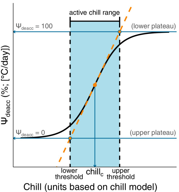
Conceptual diagram for the relationship between Ψ_deacc curve, lower threshold, upper threshold, and active chill range for deacclimation experiments and bud forcing assays in cold‐climate interspecific hybrid grapevine cultivars. The slope of the tangent line at Ψ_deacc inflection point (chill _c ) is equal to the first derivative of Ψ_deacc at chill _c , following the equation: (${\left.\frac{d{\mathrm{\Psi }}_{\text{deacc}}}{\mathrm{d}\mathit{\text{chill}}}\right|}_{\mathit{\text{chill}}=c}=\frac{-b}{\left(4\times c\right)}$), * where parameter b and parameter c are estimated by the nls() model. The lower threshold of chill occurs where the line tangent to the inflection point is equal to 0 and the upper threshold of chill occurs where the line tangent to the inflection point is equal to 100. We refer to the difference between lower and upper thresholds of chill as the active chill range. *This equation is a reduced form of the first derivative specifically at chill _c . The full derivative equation for the slope of a line tangent to any point of Ψ_deacc is: $\left.\frac{d{\mathrm{\Psi }}_{\text{deacc}}}{\mathrm{d}\mathit{\text{chill}}}\right|=-e^{(b\times \left(\ln \mathit{\text{chill}}-\ln c\right)}\times \frac{\left(b\times \left(\frac{1}{\mathit{\text{chill}}}\right)\right)}{{\left[1+e^{(b\times \left(\ln \mathit{\text{chill}}-\ln c\right)}\right]}^2}$

2.10. Effects of temperature

Deacclimation rates were analyzed for temperature effects at each level of chill unit accumulation. The effect of temperature, referred to as relative thermal contribution (H _deacc), was tested for nonlinearity by fitting a linear, quadratic and cubic model with a response variable (deacclimation rate; °C/day), and one explanatory variable (temperature; °C). A likelihood ratio test was used to compare the linear model with second‐ and third‐degree polynomials. The effect of temperature was also estimated as a logistic curve. To do this, H _deacc was estimated using the nls() function with the port algorithm, following the equation,

$$H_{\text{deacc}}=a+\frac{k_{\text{deacc},\max }-a}{1+e^{\left[g\times \left(\ln T-\ln h\right)\right]}},$$

where a, g, and h are estimated parameters and T is the temperature in °C. The parameter a is the lower limit of the logistic curve, the parameter c is the inflection point of the logistic curve and the parameter b estimates the steepness of the curve at the inflection point.

2.11. Combined effects of chill unit accumulation and temperature

The combined effect of chill unit accumulation and temperature were estimated by a combined logistic curve using the nls() function with the port algorithm, following the equation,

$$k_{\text{deacc}\left(T,\mathit{\text{Chill}}\right)}={\mathrm{\Psi }}_{\text{deacc}}\times H_{\text{deacc}}=\frac{1}{1+e^{\left[b\times \left(\ln \mathit{\text{Chill}}-\ln c\right)\right]}}\times \left[a+\frac{k_{\text{deacc},\max }-a}{1+e^{\left[g\times \left(\ln T-\ln h\right)\right]}}\right],$$

where Ψ_deacc and H _deacc are equal to the equations previously described. This combined model estimated all parameters (b, c, a, g, and h) based on Chill and T (°C) inputs.

The fits of all nonlinear curves were tested using Efron's pseudo‐R ² with the Rsq() function in the soilphysics library in R (da Silva & de Lima, 2015). A linear model was used with the complete LTE data set to evaluate the accuracy of the combined model of deacclimation predictions. In this model, change in LTE (∆LTE) is a function of the temperature (T) a bud was stored at, the quantity of chill units accumulated (Chill) before exposure to deacclimation temperatures, and the duration of exposure to deacclimation temperatures (time). The temperature and chill unit accumulation effects are incorporated in the combined model and represented within k _deacc. For accurate predictions, the β associated with k _deacc will be closer to 1 ($∆{\mathrm{LTE}}_{\left(T,\mathit{\text{Chill}}\right)}=\beta \times k_{\text{deacc}}\times \text{time}$), which means there is 1 unit change in ∆LTE for every 1‐unit change in k _deacc.

3. RESULTS

3.1. Bud forcing assays

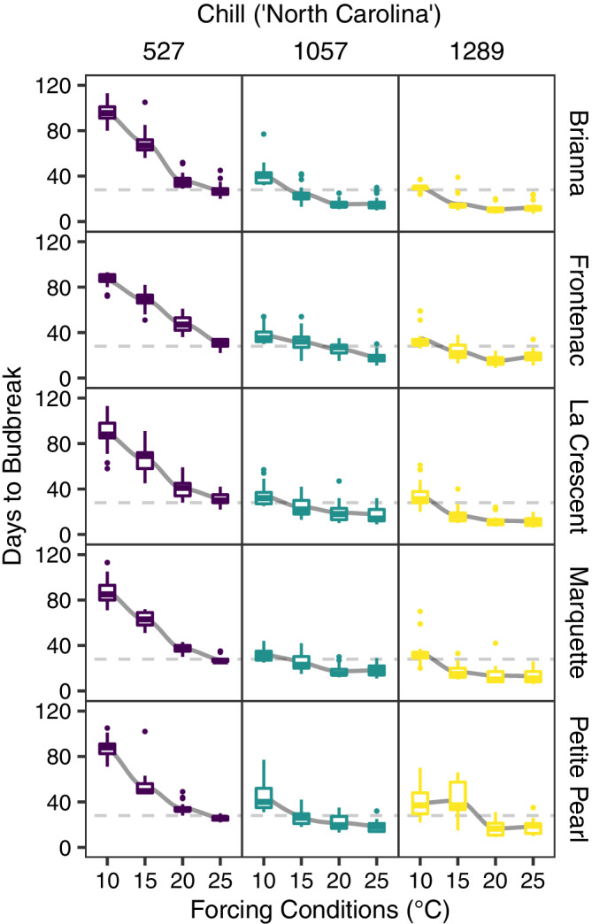
The days in forcing required to reach 50% budbreak decreased as chill units accumulated (Figure 2). For cultivars included in both years, the chill requirements were higher in Year 1 than in Year 2 according to 50% budbreak within 28 days. Chill requirements ranged from 674 to 761 (“NC”) in Year 1 and from 428 to 602 (“NC”) in Year 2.

FIGURE 2.

Days to budbreak across chill unit accumulation for deacclimation experiments and bud forcing assays in cold‐climate interspecific hybrid grapevine cultivars. Each box‐and‐whisker represents one bud forcing assay with 25 single‐node cuttings, which are colored based on chill. A trend line fit was with “loess” method of nonparametric regression (gray curves). Chill requirements based on a 28‐day threshold are labeled (intersecting, black, dashed lines). Assays were concluded after 60 days (horizontal, gray, dashed lines). Assays where less than 50% of buds grew are labeled (colored triangles at 60 days line). The active chill range based on deacclimation potential (Ψ_deacc) models is represented by shaded gray rectangles

For budbreak assays that included multiple forcing temperature treatments, days to 50% budbreak decreased for all temperatures as chill units accumulated (Figure 3). At low chill, buds incubated at warmer temperatures were faster to reach 50% budbreak compared to buds incubated at cooler temperatures. As chill increased, buds incubated at warmer temperatures generally still reached 50% budbreak in fewer days than those stored at lower but the difference was smaller across temperatures.

FIGURE 3.

Days to budbreak in forcing conditions at four temperatures across three amounts of chill unit accumulation (separated by column) in 2019–20 for deacclimation experiments and bud forcing assays in cold‐climate interspecific hybrid grapevine cultivars. A trend line was fit with “loess” method of nonparametric regression (gray curves). The horizontal gray, dashed line designates 28 days

3.2. Linear regression for deacclimation rates

Deacclimation responses were linear across time at all temperatures regardless of how much chill had accumulated (Table S1). After outliers were removed from multiple linear regression analysis, ≥84.0% of the observations were kept for each cultivar in both years. The minimum portion of observations kept for each year was 97.6% in Year 1 and 86.0% in Year 2.

The deacclimation slopes for a given temperature increased as chill units accumulated. However, deacclimation rates for experiments at chill unit accumulation >~1100 (“NC”) were slightly lower than the maximum deacclimation rate previously measured. Higher temperatures produced higher deacclimation rates as compared to lower temperatures, regardless of chill unit accumulation. There were two deviations from this trend. First, deacclimation rates were similarly small for 0, 7, and 14°C at 689 (“NC”), or low cumulative chill, in Year 1. Second, deacclimation rates were comparable for all temperatures tested (10, 15, 20, and 25°C) at 1289 (“NC”), or high cumulative chill, in Year 2.

3.3. Effects of chill unit accumulation (Ψ_deacc)

Deacclimation rates continuously increased as chill units accumulated. The continuum of deacclimation rates was quantified using a rate ratio, referred to as deacclimation potential (Ψ_deacc), by normalizing deacclimation rates across chill unit accumulation to an average of the two highest deacclimation rates. Deacclimation potential followed a logistic curve as chill units accumulated when asymptotic bounds at 0 and 100 were used as inputs for initial and final deacclimation potential, respectively (Figure 4). Pseudo‐R ² values for Ψ_deacc models were between 0.51 and 0.62 in Year 1 and between 0.79 and 0.98 in Year 2 (Table 2). The period where deacclimation potential increased correlated with chilling requirements estimated by bud forcing assays (Figure 2).

FIGURE 4.

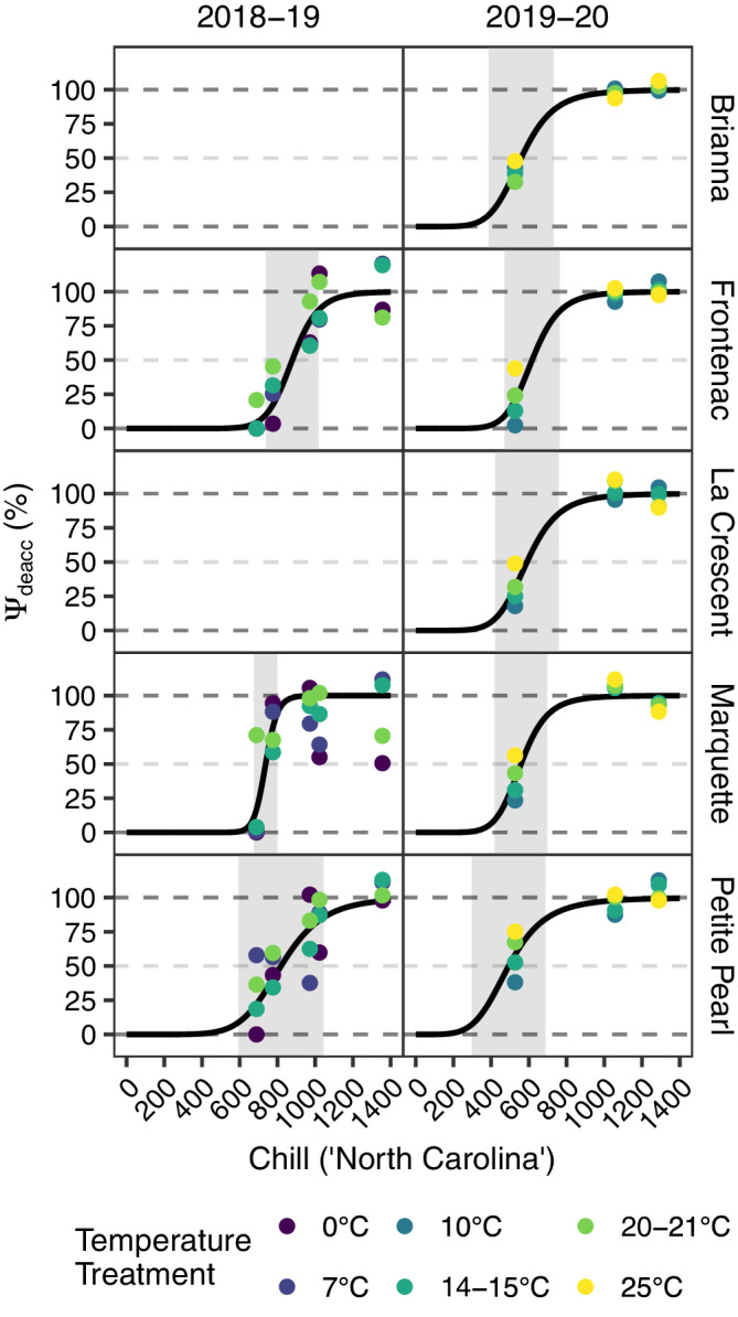
Deacclimation potential (Ψ_deacc) model predictions (black curves) and observed deacclimation potential at different temperatures (colored points) plotted across chill unit accumulation for deacclimation experiments and bud forcing assays in cold‐climate interspecific hybrid grapevine cultivars. Deacclimation potential at 0%, 50%, and 100% are indicated by horizontal, gray, dashed lines. The active chill range is represented by the gray shaded rectangles

TABLE 2.

Parameters estimated for the deacclimation potential (Ψ_deacc) model using the nls() function, including parameter b (steepness of curve), parameter c (inflection point), and pseudo‐R ² (fit of the nonlinear curve) in deacclimation experiments and bud forcing assays in cold‐climate interspecific hybrid grapevine cultivars

Deacclimation potential (Ψdeacc)
Cultivar	b	c	Pseudo‐R 2
2018–19
Frontenac	−12.6	878.7	0.816
Marquette	−23.5	737.3	0.489
Petite Pearl	−7.3	819.0	0.622
2019–20
Brianna	−6.5	559.1	0.977
Frontenac	−8.4	617.6	0.940
La Crescent	−7.0	589.8	0.926
Marquette	−8.0	558.3	0.895
Petite Pearl	−5.0	493.3	0.785

Note: Estimates were calculated separately for each cultivar and between years. Parameter c is represented in units of chill accumulation.

Three critical chill quantities were calculated based on Ψ_deacc models, including lower threshold of chill, upper threshold of chill, and active chill range. There were similar portions of Ψ_deacc that correlated with lower and upper thresholds of chills, as well as active chill range for all cultivars in both years (^e,f,g in Table 3). In terms of absolute chill units, lower and upper thresholds of chill varied between years, while “active chill range” did not (^b,c,d in Table 3). For cultivars that were included in both years of the study, the lower threshold of chill in Year 1 was similar to the upper threshold of chill in Year 2. Inflection points for Ψ_deacc curves (parameter c) also varied between years than across cultivars (Table 2). Inflection points were estimated as 746–890 (“NC”) in Year 1 and as 493‐618 (“NC”) in Year 2.

TABLE 3.

Calculations for critical chill quantities, including lower threshold of chill, upper threshold of chill, and active chill range and the relationship with deacclimation potential (Ψ_deacc) deacclimation experiments and bud forcing assays in cold‐climate interspecific hybrid grapevine cultivars

Cultivar	Slope at inflection point a	Chill lwr thr (NC chill) b	Chill upr thr (NC chill) c	Active chill range (NC chill) d	Ψdeacc at chill lwr thr (%) e	Ψdeacc at chill upr thr (%) f	Ψdeacc within active chill range (%) g
2018–19
Frontenac	0.0036	739	1018	279	10.2	86.5	76.3
Marquette	0.0080	675	800	126	11.0	87.2	76.2
Petite Pearl	0.0022	593	1045	451	8.8	85.4	76.6
2019–20
Brianna	0.0029	387	732	345	8.4	85.1	76.7
Frontenac	0.0034	471	764	293	9.3	85.8	76.5
La Crescent	0.0030	421	758	337	8.7	85.3	76.6
Marquette	0.0036	419	698	279	9.1	85.6	76.5
Petite Pearl	0.0026	298	689	391	7.3	84.4	77.1

Note: Chill quantities are listed in “North Carolina” (NC) chill units and were calculated separately for each cultivar and between years.

^a Slope of the line tangent to Ψ_deacc inflection point.

^b Chill quantity where line tangent to Ψ_deacc inflection point equals zero deacclimation potential (Ψ_deacc = 0%).

^c Chill quantity where line tangent to Ψ_deacc inflection point equals maximum deacclimation potential (Ψ_deacc = 100%).

^d Difference between lower and upper thresholds of chill.

^e Percent Ψ_deacc that corresponds with lower threshold of chill.

^f Percent Ψ_deacc that corresponds with upper threshold of chill.

^g Proportion of Ψ_deacc within lower and upper thresholds of chill.

3.4. Effects of temperature (H _deacc)

We observed a nonlinear relationship between temperature and deacclimation responses (Figure 5) as well as growth responses (Figure 3). This relationship is referred to as relative thermal contribution (H _deacc). Cultivars were pooled to evaluate the H _deacc because they followed similar trends, even though the magnitude of deacclimation rates varied among cultivars. Based on likelihood ratios tests, all linear parameters were significant for describing the H _deacc, but quadratic and cubic parameters were significant at higher chill unit accumulation levels. Relative thermal contribution (H _deacc) was also fit as a logistic curve that estimated three parameters. The y‐intercept for H _deacc curves (parameter a) was nonzero at all levels of chill except 1289 (“NC”) in Year 2, which is likely due to the absence of data for temperatures <10°C in Year 2. In the logistic model, both the inflection points (parameter h) and the steepness (parameter g) of H _deacc were lower as chill unit accumulation increased. The logistic curve was used in the model for the combined effect of chill and temperature because it had the highest fitness of all the temperature effect models (Table 4).

FIGURE 5.

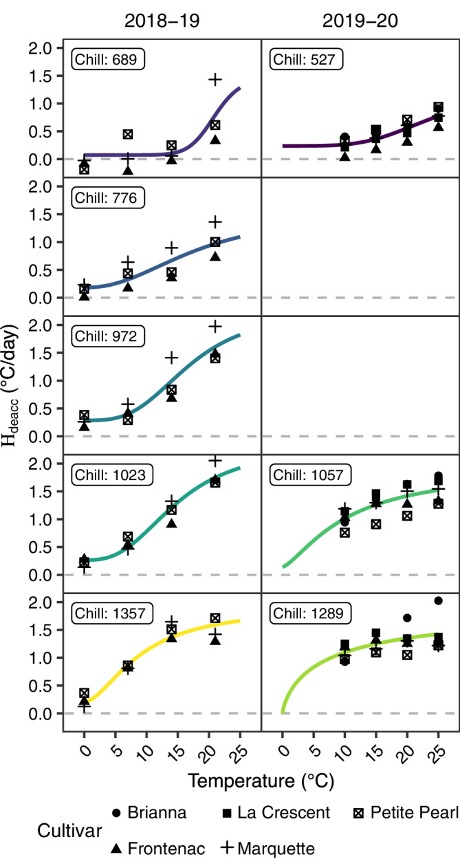
Relative thermal contribution (H _deacc) model prediction (colored curves) and observed deacclimation rate (black symbols) plotted across temperature for deacclimation experiments and bud forcing assays in cold‐climate interspecific hybrid grapevine cultivars. Predictions for each year are separated by column. Predictions for each level of chill unit accumulation are separated by row and chill unit accumulation is labeled inside the panel. Deacclimation rate minimum (0°C/day) is indicated by horizontal, gray, dashed lines

TABLE 4.

Statistical fit and logistic parameters for relative thermal contribution (H _deacc) models calculated at each level of chill (with cultivars pooled) from deacclimation experiments and bud forcing assays in cold‐climate interspecific hybrid grapevine cultivars

Relative thermal contribution (H deacc)
		Linear	Quadratic	Cubic	Logistic
Cultivar	Chill	Fit	Fit	Fit	Fit	a	g	h
2018–19
Pooled	689	0.38	0.44	0.43	0.57	0.079	−10.0	21.0
	776	0.65	0.63	0.60	0.67	0.183	−2.2	18.2
	972	0.79	0.82	0.80	0.86	0.286	−3.2	16.8
	1023	0.90	0.93	0.93	0.95	0.623	−3.0	16.2
	1357	0.82	0.91	0.93	0.92	0.205	−1.7	9.1
2019–20
Pooled	527	0.65	0.65	0.63	0.68	0.238	−4.2	23.4
	1057	0.46	0.44	0.41	0.50	0.143	−1.4	10.4
	1289	0.19	0.17	0.13	0.23	0.000	−1.0	9.4

Note: Linear, quadratic, cubic are based on R ², whereas logistic is based on Efron's pseudo‐R ²*. The logistic model parameters were calculated using the nls() function, including parameter a (y‐intercept), parameter g (steepness of curve), parameter h (inflection point). Parameter h is represented in units of temperature (°C). *Efron's pseudo‐R ² equation calculated with the following equation: $R^2=\frac{{\sum }_{i=1}^N{\left(y_i-{\widehat{\pi }}_i\right)}^2}{{\sum }_{i=1}^N{\left(y_i-\overline{y}\right)}^2}$, where $\widehat{\pi }$ is equal to model predicted probabilities.

3.5. Combined model for effects of chill unit accumulation and temperature

Estimates for the combined chill unit accumulation and temperature effects model are listed in Table 5. The Pseudo‐R ² for all cultivars ranged from 0.82 to 0.85 in Year 1 and 0.85 to 0.98 in Year 2. Statistics based on the linear model used to test the accuracy of the combined effects model are listed in Table 6, including the regression coefficient (β), R ², absolute sample size (N), and proportion of total observations (n).

TABLE 5.

Parameters estimated for the model with combined chill unit accumulation effects and temperature effects using the nls() function for deacclimation experiments and bud forcing assays in cold‐climate interspecific hybrid grapevine cultivars

Combined effect for chill unit accumulation and temperature
Cultivar	b	c	a	g	h	Pseudo‐R 2
2018–19
Frontenac	−14.6	815.2	0.388	−1.9	17.0	0.815
Marquette	−10.8	707.8	0.266	−2.6	13.1	0.854
Petite Pearl	−8.2	793.1	0.505	−2.4	16.8	0.837
2019–20
Brianna	−3.4	623.3	0.619	−2.6	16.2	0.984
Frontenac	−6.9	634.7	0.000	−5.7	7.5	0.943
La Crescent	−6.0	594.6	0.000	−2.1	6.5	0.924
Marquette	−6.0	560.6	0.388	−1.1	12.0	0.893
Petite Pearl	−2.6	476.8	0.294	−1.8	11.0	0.848

Note: Chill unit accumulation effects are represented by parameter b (steepness of curve) and parameter c (inflection point). Temperature effects are represented by parameter a (y‐intercept), parameter g (steepness of curve), and parameter h (inflection point). Fitness of the model is reported using Efron's pseudo‐R ², using the following equation: $R^2=\frac{{\sum }_{i=1}^N{\left(y_i-{\widehat{\pi }}_i\right)}^2}{{\sum }_{i=1}^N{\left(y_i-\overline{y}\right)}^2}$, where $\widehat{\pi }$ is equal to model predicted probabilities.

TABLE 6.

Linear model for evaluating accuracy of the model with combined chill unit accumulation effects (Ψ_deacc) and temperature effects, following the formula: ΔLTE_(T,Chill) = 𝛽 × k _deacc × time

Cultivar	𝛽	R 2	N (LTEs)	n (%)
2018–19
Frontenac	0.891	0.231	1429	0.995
Marquette	1.006	0.335	1446	0.999
Petite Pearl	0.824	0.249	1386	0.996
2019–20
Brianna	0.915	0.849	613	0.997
Frontenac	0.932	0.872	635	0.989
La Crescent	0.987	0.825	613	0.998
Marquette	0.983	0.833	592	0.998
Petite Pearl	0.978	0.812	594	0.992

Note: For deacclimation experiments and bud forcing assays in cold‐climate interspecific hybrid grapevine cultivars. β is the regression coefficient, R ² is coefficient of determination, N is the number of LTEs included in the model, n is the percent of LTEs included after removing outliers. Estimates were calculated separately for each cultivar and between years.

4. DISCUSSION

Dormancy, cold hardiness, and budbreak are complex processes dependent on both physiological and environmental factors. Plants synchronize the development and maintenance of dormancy, changes in cold hardiness, and timing of budbreak with the annual rhythm of seasons in order to survive in temperate climates. In this study, we describe grapevine bud deacclimation responses throughout the dormant period by integrating chill accumulation and temperature through the concept of deacclimation potential.

4.1. Effects of chill unit accumulation

4.1.1. Deacclimation responses increase continuously throughout the dormant period

Deacclimation responses gradually increased as chill units accumulated (Figure 4). The progression of deacclimation responses during the dormant season we observed differs from the traditional concept where bud deacclimation over the dormant period is a binary process where status switches from no response to a full response, corresponding to the transition from endo‐ to ecodormancy. This thinking is based on observations that buds are resistant to deacclimation during fall in endodormancy, whereas they are “physiologically primed” for deacclimation in spring, having reached ecodormancy (Arora & Taulavuori, 2016; Ferguson et al., 2014; Kalberer et al., 2006; Litzow & Pellett, 1980; Wolf & Cook, 1992). However, few studies have evaluated deacclimation at periodic intervals throughout the entire dormant period (Kovaleski et al., 2018), limiting our understanding of deacclimation dynamics during dormancy.

4.1.2. Application of deacclimation potential characterizes cold climate interspecific hybrid grapevine bud deacclimation kinetics

We quantified increasing deacclimation responses in terms of deacclimation potential (Ψ_deacc, %) (Kovaleski et al., 2018), which represents the potential to deacclimate at any temperature based on the quantity of chill units accumulated. Deacclimation potential increased as chill units accumulated following a logistic curve that can be divided into three phases (Figure 4). During the first phase, deacclimation potential is stable at approximately zero potential, meaning deacclimation does not occur, or is negligible, at any temperature. This is followed by a phase where deacclimation potential increases rapidly, meaning deacclimation rates become increasingly large as chill accumulates. In the final phase, changes in deacclimation potential slow down and deacclimation potential plateaus at 100% potential. At this point, additional chill unit accumulation does not contribute to larger deacclimation responses. When this pattern is plotted across cumulative chill, deacclimation potential represents the degree of cold hardiness loss that can occur based on chill if buds are exposed to warm temperatures.

4.1.3. The active chill range, based on deacclimation potential minimum and maximum thresholds, assesses the transition from endo‐ to ecodormancy

The phase where deacclimation potential increased overlapped the completion of endodormancy, as estimated by bud forcing assays (Figure 2). Specifically, the chill requirement estimated by bud forcing assays was slightly lower than the chill quantity where the deacclimation potential curve reached its inflection point (Ψ_deacc = 50%). An exception to this was Frontenac and Marquette in Year 2, where chilling requirement estimated by bud forcing was roughly equal to the chill quantity where deacclimation potential began to increase (between the first and second phases of deacclimation potential). Therefore, in addition to traditional bud forcing assays, deacclimation potential could be an important tool for estimating the endo‐ to ecodormancy transition, and by extension, the contribution of chill units to dormancy release. Deacclimation potential provides a quantitative assessment for dormancy status that avoids arbitrary assumptions inherent in bud forcing assays (i.e., the threshold number of days to reach 50% budbreak). Deacclimation potential also quantifies a phenotype that precedes visually observable growth. Since budbreak occurs after cold hardiness mechanisms are lost (Ferguson et al., 2014; Kovaleski et al., 2018; Salazar‐Gutiérrez et al., 2014), the amount of time needed to reach budbreak in forcing assays is a combination of the time needed for buds to fully deacclimate and the time needed for buds to visibly grow. In other words, results from bud forcing assays are confounded by deacclimation potential.

Deacclimation potential along with the parameters “lower threshold of chill,” “upper threshold of chill,” and “active chill range” can be used to determine how chilling temperatures contribute to endodormancy completion. There were similar portions of Ψ_deacc that correlated with lower and upper thresholds of chill, as well as with active chill range for all cultivars in both years (^e,f,g in Table 3), which suggests these parameters identify a consistent phenological status. In terms of absolute chill units, lower and upper thresholds of chill varied between years, while “active chill range” did not (^b,c,d in Table 3). This annual variation provides evidence that the chill accumulation model used (NC chill units, Shaltout & Unrath, 1983) is not capturing all the factors contributing to changes in deacclimation potential and, consequently, dormancy transitions. Substituting another chill model cannot correct this shortcoming either since the Pearson's correlation coefficient between the North Carolina model and other commonly used chill models is between 0.988 and 0.999 (Figure S1). Even though chilling temperatures are one of the most important environmental factors that regulate dormancy transitions and subsequent phenological development, chill models provide fairly rough mathematical approximations of temperature efficiency toward overcoming endodormancy (Fadón et al., 2020). For example, models largely do not account for negative temperature chilling, but recent studies posited negative temperatures contribute to dormancy completion (Baumgarten et al., 2021). Variations in lower threshold of chill, upper threshold of chill, and active chill range could be used to identify the most effective temperatures that contribute to changes in deacclimation potential and, therefore, dormancy transitions. As a result, Ψ_deacc, lower threshold of chill, upper threshold of chill, and active chill range introduce a valuable opportunity to improve chill models and accordingly, phenology models.

4.2. Effects of temperature

4.2.1. Deacclimation responses increase nonlinearly as temperatures increase

Deacclimation rates were greater at higher temperatures as compared to lower temperatures. Here, we refer to this relationship as relative thermal contribution (H _deacc). Both relative thermal contribution and time to budbreak followed nonlinear trends as temperature increased (H _deacc in Figure 5, time to budbreak in Figure 3). Therefore, we used a logistic curve to describe the relative thermal contribution because a minimum response is reached as temperatures decrease and a maximum response is reached as temperatures increase (Chuine, 2000; Guak & Neilsen, 2013; Kovaleski et al., 2018). While we generally observed greater deacclimation rates at higher temperatures as compared to lower temperatures, the logistic relationship accurately captures the range of temperatures where increases do not contribute to higher deacclimation responses. Changes in deacclimation rates across temperatures markedly diminished above ~15°C. Previous studies have used a linear relationship to model the effect of temperature on deacclimation (Ferguson et al., 2014; Lecomte et al., 2003), as well as the effect of temperature on plant development (Cannell & Smith, 1983; Clark & Thompson, 2010; Linkosalo et al., 2000; Richardson et al., 2018). Although this approach has been criticized due to poor predictions outside the range of temperatures modeled, it is still used as there are often only slight departures from linearity within the range of temperatures integrated into plant development models (Arnold, 1959; Keenan et al., 2020; Wolkovich et al., 2021). However, the departure from linearity can be significant below the minimum and above the optimum temperatures that stimulate plant development and deacclimation. In addition, the choice between linearity and nonlinearity influences how temperature should be integrated into models. A linear relationship implies temperature can be integrated as a change quantity (∆T), as is often done (Buermann et al., 2018; Ettinger et al., 2020). However, a nonlinear relationship between growth and temperature implies that temperature must be integrated into models in absolute quantities in order to delineate varying contributions toward a response. Therefore, it is important to recognize the nonlinear relationship between temperature and deacclimation in order to continue deepening our understanding of interdependent factors regulating deacclimation and phenology and improve growth and development models.

4.2.2. Deacclimation occurs at low temperatures that are often modeled as chilling

We observed deacclimation at temperatures as low as 0°C, the minimum temperature treatment included in our study. To accommodate this in the H _deacc model, the y‐intercept (parameter a) was allowed to vary rather than fixed at 0 to allow estimation of deacclimation at 0°C (Figure 5, Table 4). To our knowledge, no previous studies examining deacclimation in grapevine have reported deacclimation at 0°C. However, some evidence of low‐temperature deacclimation in the literature can be found. For example, the lowest base temperature parametrized in a cold hardiness prediction model for 23 grapevine genotypes grown in Washington was 3°C (Ferguson et al., 2014). In addition, deacclimation was reported at temperatures as low as 2°C for four grapevine species grown in New York (Kovaleski et al., 2018). Deacclimation at chilling temperatures has not been thoroughly accounted for despite several previous studies that have explored the phenomenon (Arora et al., 2004; Cragin et al., 2017; Slater et al., 1991). Based on our results, future studies exploring bud deacclimation in temperate woody plants should include temperatures close to the freezing point, especially for species with a propensity to deacclimate at low temperatures, such as cold climate hybrid grapevines. Ultimately, deacclimation at low temperatures demonstrates the importance for integrating low‐temperatures contributions to growth when modeling phenology.

4.3. Combined effects of chill unit accumulation and temperature

4.3.1. Balance between interacting factors to determine deacclimation responses

Deacclimation responses are conditional in response to both chill unit accumulation and temperature (Figure 6). Deacclimation responses increased at all temperatures as chill units accumulated, until the deacclimation potential reached its maximum, at which point additional chill units did not increase the rate of deacclimation. Therefore, temperatures within the chilling range (i.e., 0–7°C) occurring in the spring may lead to no or minimal increases in deacclimation potential (Ψ_deacc), and instead directly promote deacclimation responses. This leads to the slight reductions in time to budbreak seen at >1000 chill units (Figure 2).

FIGURE 6.

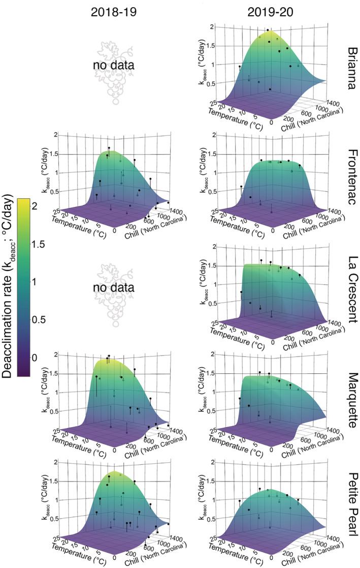
Predicted deacclimation rates (colored surface) plotted with observed deacclimation rates (black points) for deacclimation experiments and bud forcing assays in cold‐climate interspecific hybrid grapevine cultivars. The difference between predicted and observed deacclimation rate is represented by vertical black lines. Predictions were calculated using the model that combined chill unit accumulation effects and temperature effects

Differences in deacclimation rates across temperatures were small at low chill unit accumulation. However, as chill unit accumulation increased, deacclimation rates increased at a higher rate in the high temperatures treatments than in the low temperatures treatments. Therefore, deacclimation potential, as a quantitative description of dormancy, evenly regulates deacclimation rates for all temperatures. Based on the nonlinear relationship between temperature and deacclimation, there are different, yet proportional, increases in deacclimation rates across temperature as chill accumulates.

4.3.2. Deacclimation responses can be modeled based on combined chill and temperature effects

The model that combines chilling accumulation and temperature effects accurately represents the overall changes in deacclimation rates. The linear model used to test the accuracy of the combined effects model had a regression coefficient (β) ranging from 0.824 to 1.006 across all cultivars in both years (Table 6). This is exceptional, considering a β = 1 would indicate there is 1‐unit change in ∆LTE for every 1‐unit change in k _deacc. The low R ² values associated with the 2018–19 models indicate there was a wide range of LTEs throughout the deacclimation experiments. However, the model still accurately represented the kinetics for changes in deacclimation rates since the regression coefficients are near one. Therefore, the individual effects of chill unit accumulation and temperature on deacclimation can be combined into a single model that quantifies deacclimation kinetics throughout the dormant period and can guide improvements to models predicting cold hardiness fluctuations and phenological development in woody perennials.

5. CONCLUSION

Descriptions of the mechanisms by which plants deacclimate, the factors regulating deacclimation, and the seasonal rhythm of deacclimation kinetics are necessary to understand the freeze injury risks that perennial plants face in climates where freezing temperatures occur. In this study, we have described the effects of two factors, chill unit accumulation and temperature, on deacclimation responses. Future studies describing dormancy transitions and chilling requirements should include an assessment of deacclimation potential (Ψ_deacc) in their experimental designs because it provides an additional method for quantifying dormancy transitions. Most importantly, deacclimation potential quantifies a physiological bud phenotype that precedes externally visible bud growth, the necessary observation in bud forcing assays. In addition, deacclimation potential characterizes a chill range where physiological bud responses continuously increase until they reach their maximum potential. This provides an opportunity to identify the most effective temperatures contributing to the dormancy transition, thereby improving chill models. Relative thermal contribution (H _deacc) demonstrates that temperature, as a variable in predictive models, needs to be integrated in total units rather than units of change (∆T). Furthermore, in our study, deacclimation occurred at temperatures as low as 0°C, which has not been observed in grapevine before. Further studies are necessary to evaluate deacclimation at low temperatures in other woody plants. This could necessitate adjustments to base temperatures in phenology prediction models for plants that deacclimate at low temperatures. Finally, in this study, we have demonstrated that the effects of chill unit accumulation and temperature can be combined in a predictive model that accurately describes changes in deacclimation responses across the dormant period. This deacclimation model can guide the development of new cold hardiness prediction models, as well as improvements to existing models.

AUTHOR CONTRIBUTIONS

Study conception and design were completed by Amaya Atucha, Beth Ann Workmaster, and Michael North. Experiment execution, data collection, and data analysis were completed by Michael North. Data interpretation and manuscript writing were completed by Amaya Atucha, Beth Ann Workmaster, and Michael North.

Supporting information

Appendix S1 Additional supporting information may be found in the Supporting Information section at the end of this article online.

Figure S1 Comparison of chill models

Table S1 Linear regression statistics

North, M. , Workmaster, B.A. & Atucha, A. (2022) Effects of chill unit accumulation and temperature on woody plant deacclimation kinetics. Physiologia Plantarum, 174(3), e13717. Available from: 10.1111/ppl.13717

DATA AVAILABILITY STATEMENT

The data that support the findings of this study are available from the corresponding author upon reasonable request.

REFERENCES

- Arnold, C.Y. (1959) The determination and significance of the base temperature in a linear heat unit system. American Society for Horticultural Science, 74, 430–445. [Google Scholar]
- Arora, R. & Rowland, L.J. (2011) Physiological research on winter‐hardiness: deacclimation resistance, reacclimation ability, photoprotection strategies, and a cold acclimation protocol design. HortScience, 46, 1070–1078. [Google Scholar]
- Arora, R. , Rowland, L.J. , Ogden, E.L. , Dhanaraj, A.L. , Marian, C.O. , Ehlenfeldt, M.K. et al. (2004) Dehardening kinetics, bud development, and dehydrin metabolism in blueberry cultivars during deacclimation at constant, warm temperatures. Journal of the American Society for Horticultural Science, 129, 667–674. [Google Scholar]
- Arora, R. & Taulavuori, K. (2016) Increased risk of freeze damage in woody perennials VIS‐À‐VIS climate change: importance of deacclimation and dormancy response. Frontiers in Environmental Science, 4, 1–7. [Google Scholar]
- Baumgarten, F. , Zohner, C.M. , Gessler, A. & Vitasse, Y. (2021) Chilled to be forced: the best dose to wake up buds from winter dormancy. The New Phytologist, 230, 1366–1377. [DOI] [PubMed] [Google Scholar]
- Buermann, W. , Forkel, M. , O'Sullivan, M. , Sitch, S. , Friedlingstein, P. , Haverd, V. et al. (2018) Widespread seasonal compensation effects of spring warming on northern plant productivity. Nature, 562, 110–114. [DOI] [PubMed] [Google Scholar]
- Camargo Alvarez, H. , Salazar‐Gutiérrez, M. , Zapata, D. , Keller, M. & Hoogenboom, G. (2018) Time‐to‐event analysis to evaluate dormancy status of single‐bud cuttings: an example for grapevines. Plant Methods, 14, 1–13. [DOI] [PMC free article] [PubMed] [Google Scholar]
- Campoy, J.A. , Ruiz, D. & Egea, J. (2011) Dormancy in temperate fruit trees in a global warming context: a review. Scientia Horticulturae, 130, 357–372. [Google Scholar]
- Cannell, M.G.R. & Smith, R.I. (1983) Thermal time, chill days and prediction of budburst in Picea sitchensis . Journal of Applied Ecology, 20, 951–963. [Google Scholar]
- Charrier, G. , Bonhomme, M. , Lacointe, A. & Améglio, T. (2011) Are budburst dates, dormancy and cold acclimation in walnut trees (Juglans regia L.) under mainly genotypic or environmental control? International Journal of Biometeorology, 55, 763–774. [DOI] [PubMed] [Google Scholar]
- Chuine, I. (2000) A unified model for budburst of trees. Journal of Theoretical Biology, 207, 337–347. [DOI] [PubMed] [Google Scholar]
- Clark, R.M. & Thompson, R. (2010) Predicting the impact of global warming on the timing of spring flowering. International Journal of Climatology, 30, 1599–1613. [Google Scholar]
- Cook, R.D. (1977) Detection of influential observation in linear regression detection of influential observation in linear regression. Technometrics, 19, 15–18. [Google Scholar]
- Cooke, J.E.K. , Eriksson, M.E. & Junttila, O. (2012) The dynamic nature of bud dormancy in trees: environmental control and molecular mechanisms. Plant, Cell and Environment, 35, 1707–1728. [DOI] [PubMed] [Google Scholar]
- Coombe, B.G. (1995) Growth stages of the grapevine: adoption of a system for identifying grapevine growth stages. Australian Journal of Grape and Wine Research, 1, 104–110. [Google Scholar]
- Coville, F. (1920) The influence of cold in stimulating the growth of plants. Proceedings of the National Academy of Sciences of the United States of America, 6, 434–435. [DOI] [PMC free article] [PubMed] [Google Scholar]
- Cragin, J. , Serpe, M. , Keller, M. & Shellie, K. (2017) Dormancy and cold hardiness transitions in winegrape cultivars chardonnay and cabernet sauvignon. American Journal of Enology and Viticulture, 68, 195–202. [Google Scholar]
- da Silva, A.R. & de Lima, R.P. (2015) Soilphysics: an R package to determine soil preconsolidation pressure. Computers and Geosciences, 84, 54–60. [Google Scholar]
- Deshpande, G. & Jia, H. (2020) Multi‐level clustering of dynamic directional brain network patterns and their behavioral relevance. Frontiers in Neuroscience, 13, 1–22. [DOI] [PMC free article] [PubMed] [Google Scholar]
- Erez, A. , Fishman, S. , Linsley‐Noakes, G.C. & Allan, P. (1990) The dynamic model for rest completion in peach buds. Acta Horticulturae, 276, 165–174. [Google Scholar]
- Ettinger, A.K. , Chamberlain, C.J. , Morales‐Castilla, I. , Buonaiuto, D.M. , Flynn, D.F.B. , Savas, T. et al. (2020) Winter temperatures predominate in spring phenological responses to warming. Nature Climate Change, 10, 1137–1142. [Google Scholar]
- Fadón, E. , Fernandez, E. , Behn, H. & Luedeling, E. (2020) A conceptual framework for winter dormancy in deciduous trees. Agronomy, 10, 241. [Google Scholar]
- Ferguson, J.C. , Moyer, M.M. , Mills, L.J. , Hoogenboom, G. & Keller, M. (2014) Modeling dormant bud cold hardiness and Budbreak in twenty‐three Vitis genotypes reveals variation by region of origin. American Journal of Enology and Viticulture, 65, 59–71. [Google Scholar]
- Fishman, S. , Erez, A. & Couvillon, G.A. (1987a) The temperature dependence of dormancy breaking in plants: computer simulation of processes studied under controlled temperatures. Journal of Theoretical Biology, 126, 309–321. [Google Scholar]
- Fishman, S. , Erez, A. & Couvillon, G.A. (1987b) The temperature dependence of dormancy breaking in plants: mathematical analysis of a two‐step model involving a cooperative transition. Journal of Theoretical Biology, 124, 473–483. [Google Scholar]
- Gariglio, N. , González Rossia, D.E. , Mendow, M. , Reig, C. & Agusti, M. (2006) Effect of artificial chilling on the depth of endodormancy and vegetative and flower budbreak of peach and nectarine cultivars using excised shoots. Scientia Horticulturae, 108, 371–377. [Google Scholar]
- Gu, L. , Hanson, P.J. , Mac, P.W. , Kaiser, D.P. , Yang, B. , Nemani, R. et al. (2008) The 2007 eastern US spring freeze: increased cold damage in a warming world? Bioscience, 58, 253–262. [Google Scholar]
- Guak, S. & Neilsen, D. (2013) Chill unit models for predicting dormancy completion of floral buds in apple and sweet cherry. Horticulture Environment and Biotechnology, 54, 29–36. [Google Scholar]
- Hanninen, H. (2013) Modeling bud dormancy release in trees from cool and temperate regions. Acta Forestalia Fennica, 213, 47. [Google Scholar]
- Hänninen, H. & Kramer, K. (2007) A framework for modelling the annual cycle of trees in boreal and temperate regions. Silva Fennica, 41, 167–205. [Google Scholar]
- IPCC . (2014) Climate change 2013. The physical science basis. Cambridge: Cambridge University Press. [Google Scholar]
- Junttila, O. & Hänninen, H. (2012) The minimum temperature for budburst in Betula depends on the state of dormancy. Tree Physiology, 32, 337–345. [DOI] [PubMed] [Google Scholar]
- Kalberer, S.R. , Wisniewski, M. & Arora, R. (2006) Deacclimation and reacclimation of cold‐hardy plants: current understanding and emerging concepts. Plant Science, 171, 3–16. [Google Scholar]
- Keenan, T.F. , Richardson, A.D. & Hufkens, K. (2020) On quantifying the apparent temperature sensitivity of plant phenology. The New Phytologist, 225, 1033–1040. [DOI] [PubMed] [Google Scholar]
- Kovaleski, A.P. & Londo, J.P. (2019) Tempo of gene regulation in wild and cultivated Vitis species shows coordination between cold deacclimation and budbreak. Plant Science, 287, 110178. [DOI] [PubMed] [Google Scholar]
- Kovaleski, A.P. , Reisch, B.I. & Londo, J.P. (2018) Deacclimation kinetics as a quantitative phenotype for delineating the dormancy transition and thermal efficiency for budbreak in Vitis species. AoB PLANTS, 10, 1–12. [DOI] [PMC free article] [PubMed] [Google Scholar]
- Lang, G.A. (1987) Dormancy: a new universal terminology. HortScience, 22, 817–820. [Google Scholar]
- Lang, G.A. , Early, J.D. , Martin, G.C. & Darnell, R.L. (1987) Endo‐, para‐, and ecodormancy: physiological terminology and classification for dormancy research. HortScience, 22, 371–377. [Google Scholar]
- Lecomte, C. , Giraud, A. & Aubert, V. (2003) Testing a predicting model for frost resistance of winter wheat under natural conditions. Agronomie, 23, 51–66. [Google Scholar]
- Levitt, J. (1980) High‐temperature or heat stress. In: Responses of plants to environmental stresses: chilling, freezing, and high temperature stresses. New York, NY: Academic Press. [Google Scholar]
- Linkosalo, T. , Carter, T.R. , Hakkinen, R. & Hari, P. (2000) Predicting spring phenology and frost damage risk of Betula spp. under climatic warming: a comparison of two models. Tree Physiology, 20, 1175–1182. [DOI] [PubMed] [Google Scholar]
- Litzow, M. & Pellett, H. (1980) Relationship of rest to dehardening in red‐osier dogwood. HortScience, 15, 92–93. [Google Scholar]
- Londo, J.P. & Johnson, L.M. (2014) Variation in the chilling requirement and budburst rate of wild Vitis species. Environmental and Experimental Botany, 106, 138–147. [Google Scholar]
- McDowall, L.M. & Dampney, R.A.L. (2006) Calculation of threshold and saturation points of sigmoidal baroreflex function curves. American Journal of Physiology – Heart and Circulatory Physiology, 291, 2003–2007. [DOI] [PubMed] [Google Scholar]
- Mills, L.J. , Ferguson, J.C. & Keller, M. (2006) Cold‐hardiness evaluation of grapevine buds and cane tissues. American Journal of Enology and Viticulture, 57, 194–200. [Google Scholar]
- North, M. , Workmaster, B.A. & Atucha, A. (2021) Cold hardiness of cold climate interspecific hybrigrapevines grown in a cold climate region. American Journal of Enology and Viticulture, 72, 318–327. [Google Scholar]
- Pagter, M. & Arora, R. (2013) Winter survival and deacclimation of perennials under warming climate: physiological perspectives. Physiologia Plantarum, 147, 75–87. [DOI] [PubMed] [Google Scholar]
- Richardson, A.D. , Hufkens, K. , Milliman, T. , Aubrecht, D.M. , Furze, M.E. , Seyednasrollah, B. et al. (2018) Ecosystem warming extends vegetation activity but heightens vulnerability to cold temperatures. Nature, 560, 368–371. [DOI] [PubMed] [Google Scholar]
- Richardson, E.A. , Sceley, S.D. & Walker, D.R. (1974) A model for estimating the completion of rest for “Redhaven” and “Elberta” peach trees. HortScience, 9, 331–332. [Google Scholar]
- Salazar‐Gutiérrez, M.R. , Chaves, B. , Anothai, J. , Whiting, M. & Hoogenboom, G. (2014) Variation in cold hardiness of sweet cherry flower buds through different phenological stages. Scientia Horticulturae, 172, 161–167. [Google Scholar]
- Shaltout, A.D. & Unrath, C.R. (1983) Rest completion prediction model for “Starkrimson delicious” apples. Journal of American Society for Horticultural Science, 108, 957–961. [Google Scholar]
- Slater, J.V. , Warmund, M.R. , George, M.F. & Ellersieck, M.R. (1991) Deacclimation of winter hardy “Seyval blanc” grape tissue after exposure to 16°C. Scientia Horticulturae, 45, 273–285. [Google Scholar]
- USDA Plant Hardiness Zone Map . (2012) Agricultural Research Service. Corvallis, OR: U.S. Department of Agriculture. Accessed from https://planthardiness.ars.usda.gov/ [Google Scholar]
- Weinberger, J.H. (1950) Chilling requirements of peach varieties. Proceedings of the American Society for Horticultural Science, 56, 122–128. [Google Scholar]
- Wolf, T.K. & Cook, M.K. (1992) Seasonal deacclimation patterns of three grape cultivars at constant, warm temperature. American Journal of Enology and Viticulture, 43, 171–179. [Google Scholar]
- Wolkovich, E.M. , Auerbach, J. , Chamberlain, C.J. , Buonaiuto, D.M. , Ettinger, A.K. , Morales‐Castilla, I. et al. (2021) A simple explanation for declining temperature sensitivity with warming. Global Change Biology, 27, 4947–4949. [DOI] [PubMed] [Google Scholar]
Associated Data
This section collects any data citations, data availability statements, or supplementary materials included in this article.
Supplementary Materials