Abstract
Change Point Detection (CPD) is the problem of discovering time points at which the behavior of a time series changes abruptly. In this paper, we present a novel real-time nonparametric change point detection algorithm called SEP, which uses Separation distance as a divergence measure to detect change points in high-dimensional time series. Through experiments on artificial and real-world datasets, we demonstrate the usefulness of the proposed method in comparison with existing methods
Index Terms—: Activity transition detection, change detection algorithms, Separation distance, smart homes, time series data
1. Introduction
Change Point Detection (CPD) is the problem of discovering time points at which the behavior of a time series changes abruptly. CPD is a well-established area and has been studied over the past several decades in the fields of data mining, statistics, and computer science. CPD finds application in a broad range of real-world problems such as medical condition monitoring [1], climate change detection [2][3], speech recognition [4][5], image analysis [6], and human activity analysis [7][8][9]. Many algorithms have been designed, enhanced, and adapted for change point detection. These techniques include both supervised and unsupervised methods, chosen based on the desired outcome of the algorithm. While change point detection is a well-investigated field, research on real-time CPD is more recent and rare. In contrast with traditional CPD approaches, real-time CPD algorithms run concurrently with the processes they are monitoring, processing each data point as it becomes available. The goal is to detect a change point as soon as possible after it occurs, ideally before the next data point arrives [10]. However, online algorithms place different requirements on the amount of new data that must be viewed before a change can be detected.
Recently, direct density ratio change point detection algorithms have been introduced which address these challenges [11]. These algorithms detect change points between two consecutive windows of data by estimating their probability density ratio based on the assumption that the probability densities of two consecutive windows are the same if they belong to the same state. The goal of this paper is to further advance this line of research by improving the current start-of-the-art method and introducing a new unsupervised algorithm for change point detection in time-series data which we call SEParation change point detection, or SEP. The proposed approach can be applied to data of arbitrary dimensionality and detects change points in near real time. Our novel SEP change point detection method employs new probability metrics and improves the performance of existing density ratio-based change point detection algorithms by providing a more sensitive change score. As we demonstrate, this method results in detection of more subtle and a greater variety of changes.
This paper offers several contributions to change point detection. We first introduce a new CPD method built on the notion of SEParation distance and contrast the approach with existing CPD methodologies. Second, we further complete the set of relationships that have been defined between existing probability metrics by relating the Separation distance and Pearson metrics. Finally, we evaluate and implement SEP using artificial datasets and benchmark datasets. We also evaluate SEP on a complex multidimensional real-world application, namely detecting changes in sensor-based human behavior data. CPD offers several valuable opportunities in such a setting, including health event detection, breakpoint detection, and activity segmentation [12][13]. Detecting change points in smart home sensor data is valuable for detecting health events and identifying activity transition points. Our experimental results on real and synthetic data indicate that SEP performs as well or better than existing methods at classical CPD and offers new features that are valuable for complex real-time problems such as smart home-based human behavior analysis.
2. Background
In order to introduce our SEP method, we first present definitions of key terms with a formulation of the change point detection problem and probability functions that we use throughout the paper. We also review existing change point detection methods, focusing primarily on those that employ density ratio methods.
2.1. Definitions and Problem Formulation
We begin this discussion with definitions of time series data and change points.
Definition 1. A time series data stream is an infinite sequence of elements S={x1, …, xi, …}, where xi is a d-dimensional data vector arriving at time stamp i [14].
Time series data reflects the current status of a process or system. When the parameters governing the process do not change for a period of time, the process and corresponding time series subsequence remains in a single state. Two consecutive distinct states are distinguished by a change point. Indeed, a change point represents a transition between different states in a process that generates the time series data.
Definition 2. If X is a random variable defined on , for every subset B of we can define a measure μX that reflects the probability density function of the subset. This function, shown in Equation 1, is used by some methods to compare data distributions and detect change points.
| (1) |
where (, B, μX) is a probability space and P is the probability of X in B. If X is continuous, we can define probability density function such that
| (2) |
Definition 3. Given a time series S, we assume time stamp t is a change point if the probability density function f created from sliding-window data observed before and after t are different either in terms of the type of the function or the parameters characterizing the function change. Let {xm,, …, xk, …, xn} be a sequence of time series data points that are observed as part of times series S. Change point detection (CPD) can be defined as the problem of hypothesis testing between two alternatives consisting of the null hypothesis H0: “No change occurs in time series S at time stamp k*” and the alternative hypothesis HA: “A change occurs in time series S at time stamp k*” [15][16].
H0: fxm ≈ … ≈ fxk* ≈ … ≈ fxn
HA: There exists m<k*<n such that
where fxi is the probability density function of the sliding window starting at point xi and k* is a time in the series where the process is changing states.
A change point detection algorithm is an algorithm that utilizes information about time series data to determine if and where change points occur. Change point detection algorithms typically need to consider data before and after potential change points to make this determination. As a result, we also want to consider the efficiency with which these decisions can be made. This leads us to the next definition.
Definition 4. A change point detection algorithm can be said to perform in ε-real time when the algorithm makes a decision about a change point occurring at time k* after a delay of ε time points. In other words, the ε-real time algorithm needs to examine data points xk*, xk*+1,.., xk*+ ε in order to decide whether or not k* is a change point. An offline algorithm can then be viewed as ∞-real time and a completely-online algorithm is 0-real time because for every data point, it can predict whether or not a change point occurs before the new data point. Because of their increased detection efficiency, algorithms that operate with smaller ε values may lead to more responsive change point detection applications.
2.2. Existing CPD Methods
Change point detection algorithms have been studied for decades and there are multiple techniques described in the literature. Figure 1 provides an overview of existing change point detection algorithms. Both supervised and unsupervised methods have been used to solve CPD problems. When a supervised approach is employed for change point detection, machine learning algorithms can be trained as either binary or multi-class classifiers. If the number of possible process states is specified, the change point detection algorithm may be trained to find each state boundary, making it a multi-class problem. A sliding window moves through the data, considering each possible division between two data points as a possible state boundary or change point [17][18][19]. While this approach has a simpler training phase, a sufficient amount and diversity of training data needs to be provided to represent not only each individual state class but also all possible transitions from one state to another. On the other hand, detecting each state separately may provide sufficient information to find both the nature and the amount of detected change.
Fig. 1.
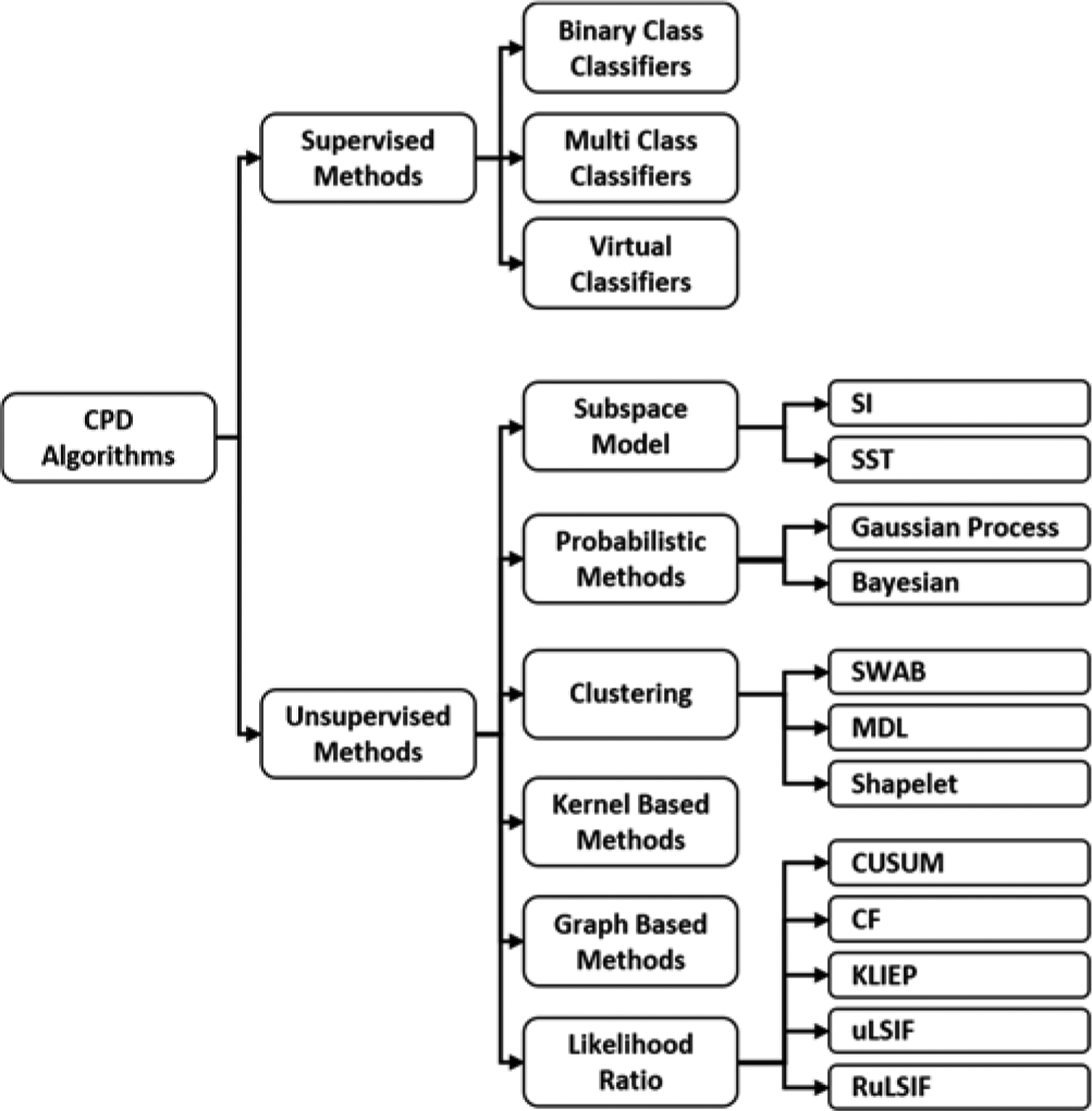
Overview of change point detection algorithms.
An alternative is to treat change point detection as a binary classification problem, where all of the possible state transition (change point) sequences represent one class and all of the within-state sequences represent a second class. While only two classes need to be learned in this case, this is a much more complex learning problem if the number of possible types of transitions is large [7][20][21]. In addition to detecting changes, a virtual classifier can be used to also interpret the change that occurs between two consecutive windows [22]. For each pair of consecutive windows, the virtual classifier attaches a hypothetical label (+1) to samples from the first window and (−1) to samples from the second window. The algorithm then trains a virtual classifier (VC) using any supervised method that generates human-interpretable rules (e.g., a decision tree) based on the labeled data points. If there is a change point between two windows, the classifier should correctly classify it and the classification accuracy should be significantly higher than random noise. Once the change point is detected, the classifier is re-trained using all of the samples in the two neighboring windows. If some features play a dominant role in the classifier, then they are the ones that characterize the difference.
Unsupervised learning algorithms are typically used to discover patterns (and pattern changes) in unlabeled data. In the context of change point detection, such algorithms can be used to segment time series data by finding change points based on statistical features of the data. Unsupervised segmentation is attractive because it may handle a variety of different situations without requiring prior training for each state and state change. One traditional solution is subspace modelling, which represents a time series using state spaces and detects change points by identifying the state space distances. This approach has a strong connection with a system identification method, which has been thoroughly studied in control theory. Assuming we have two consecutive sliding windows, Subspace Identification (SI) [23] estimates an extended observability matrix based on a state space model that is generated for each sliding window and calculates the gap between subspaces as a measure of the change. Singular Spectrum Transformation (SST) [24] is another similar approach which calculates distance-based change point scores by comparing singular spectrums of two trajectory matrices for consecutive windows.
Probabilistic methods estimate probability distributions for each new window based on the data that has been observed since the previous candidate change point. As an example, the Bayesian algorithm designed by Adams and McKay [25] uses Bayes’ theorem to estimate a current state’s run-length (rt) which represents the time that has elapsed in the time series since the last change point. Given the run length at a time point t, the run length at the next time point t+1 can either reset back to 0 (if a change point occurs at time t) or increase by 1 (if the current state continues for one more time unit). Using a different type of probabilistic approach, the Gaussian Process (GP) algorithm by Saatçi, et al. [26] defines a time series data point as noisy Gaussian distribution function values. Given a time series, the GP function will make a normal distribution-based prediction of the data point at time t. Change points are detected by comparing the predicted and actual data point values.
Clustering methods, which are very popular for change point detection, group time series data into clusters of similar data points that represent their respective states and find changes by identifying differences between features of the cluster states. Although it was designed as a time series segmentation algorithm, SWAB (Sliding Window and Bottom-up) [27] exemplies this approach and can be used for change detection. SWAB detects change points by combining sliding window and bottom-up methods. The original bottom-up approach first treats each data point as a separate subsequence, then merges subsequences with an associated merge cost until the stopping criteria is met. Extending this further, SWAB also maintains a buffer of size w to store enough data for 5–6 clusters. The bottom-up method is applied to the data in the buffer as well as the leftmost resulting cluster and any corresponding detected change point is reported. The data corresponding to the reported subsequence are removed from the buffer and replaced with the next data in the series. In contrast, the MDL-based change point detection [28] is a bottom-up greedy search over the space of clusters which can include subsequences of different lengths and does not require the number of clusters to be specified. The Shapelet-based clustering method [29] is a greedy search algorithm which attempts to cluster the data based on the shape of the entire time series. This method searches for a u-shapelet which can separate and remove a time series state from the rest of the dataset. The algorithm iteratively repeats this search among the remaining data until no data remains to be separated.
Kernel-based methods [30] map observations onto a higher-dimensional feature space and detect change points by comparing the homogeneity of each subsequence. Graph-based techniques have been used as well. The graph-based technique of Chen and Zhang [15] is a non-parametric approach that represents time series as a graph in which its nodes are time series data points. This algorithm then applies a two-sample statistical test to detect change points based on the graph representation.
In this research, we focus on density ratio change point detection techniques. We narrow our approach to these methods because they are unsupervised, can detect change points in near-real time, and have demonstrated good performance in the literature. These CPD techniques utilize density ratios based on the observation that the probability density of two consecutive windows are the same if they belong to the same state. A typical statistical analysis of change-point detection analyzes the probability distributions of data before and after a candidate change point, and identifies the candidate as a change point if the two distributions are significantly different. One of the early reported density ratio methods is cumulative sum (CUSUM) [31] which accumulates deviations relative to a specified target of incoming measurements and indicates that a change point exists when the cumulative sum exceeds a specified threshold. The Change Finder (CF) algorithm [32] reduces the problem of change point detection into time series-based outlier detection. Since these methods rely on pre-designed parametric models and they are less flexible in real-world change point detection scenarios, some recent studies introduce more flexible non-parametric variations by estimating the ratio of probability densities directly without needing to perform the actual density estimations. These density ratio-based approaches to change point detection are among the most popular approaches and form the basis of our SEP method described in the next section. The rationale of this density-ratio estimation idea is that knowing the two densities implies knowing the density ratio. However, the inverse is not true: knowing the ratio does not necessarily imply knowing the two densities because such decomposition is not unique. Thus, direct density-ratio estimation is substantially simpler than density estimation. Following this idea, methods of direct density-ratio estimation have been developed [33][11].
3. SEP Change Point Detection
Recent studies show compared with other change-point detection methods, density ratio based algorithms offer several advantages for real world problems [11][34]. Assuming two probability densities, ft(x) and ft−1(x), corresponding to two consecutive windows, each with length n, density ratio-based CPD methods use dissimilarity measures as a measure of difference between them to determine whether or not there exists a change point between these two windows. These methods model the density ratio by a non-parametric Gaussian kernel model, shown in Equations 3 and 4.
| (3) |
| (4) |
In these equations, θ=(θ1, …, θn)T represents the set of parameters for the ratio function to be learned from existing data points in the current windows, and σ>0 represents the kernel parameter. In the training phase, the parameters θ are determined for each window so that a chosen dissimilarity measure is minimized. Given a density-ratio estimator gt(x), a dissimilarity measure between windows is calculated during the test phase as a change point score. Since the higher the change point score is, the more likely the point is a change point [33][11], these methods identify change points by comparing scores to a threshold. Existing direct density ratio change point detection algorithms use different dissimilarity measures. This means each method uses different models and optimization processes, thus the change point score calculation will change based on these choices.
One of the first direct density ratio CPD methods, the Kullback-Leibler importance estimation procedure (KLIEP) [35], estimates the density ratio using Kullback-Leibler (KL) divergence. KL divergence, defined in Equation 5, is a popular choice for the dissimilarity measure.
| (5) |
This problem is a convex optimization problem, so the unique global optimal solution θ can be obtained, for example, by a gradient projection method. The resulting approximation of KL divergence is given in Equation 6 [35]. The notation and represent the estimator of KL and g, respectively.
| (6) |
Another direct density ratio estimator is uLSIF (Unconstrained Least-Squares Importance Fitting) [36], which uses Pearson (PE) divergence as a dissimilarity measure, as shown in Equation 7.
| (7) |
As part of the uLSIF training criterion, the density-ratio model is fitted to the true density ratio under the squared loss. An approximator of the PE divergence is shown in Equation 8.
| (8) |
Depending on the value of the second window density function, the density-ratio value can be unbounded. To overcome this problem, α-relative PE divergence for 0≤α<1 is used as a dissimilarity measure in an approach known as Relative uLSIF (RuLSIF) [11]. The RuLSIF dissimilarity measure is defined in Equation 9.
| (9) |
The α-relative density ratio is reduced to a plain density ratio if α=0 [11][37].
As mentioned, one of the key elements for density ratio-based methods is the choice of dissimilarity or divergence measure function. This function computes the difference between the probability density functions for two consecutive windows of data.
A function d(·, ·) provides an appropriate measure of difference if and only if the following four conditions are satisfied [38]:
Non-negativity: ∀ x, y, d(x, y) ≥ 0
Non-degeneracy: d(x, y) = 0 ↔ x = y
Symmetry: ∀ x, y, d(x, y) = d(y, x)
Triangle inequality: ∀ x, y, z, d(x, z) ≤ d(x, y) + d(y, z)
A dissimilarity / divergence is a pseudo-difference if it violates some of the above conditions. There are several metrics available to quantify the difference between probability density functions in change point detection algorithms. For example, the KLIEP change point detection algorithm [35] uses the Kullback-Leibler divergence for its metric, while both uLSIF [36] and RuLSIF [11] use Pearson divergence. The question is, how does one choose an optimal metric? Alternatively, what are the issues that affect a metric’s desirability? To answer these questions and determine if there is another potential metric that can further improve change point detection, we start by investigating existing metrics and their relationships.
Table 1 lists different probability metrics found in the literature. In this table, μ and ν represent two probability measures while f and q represent their corresponding probability density functions based on Definition 2. Figure 2 pictorially describes the relationship between these metrics. A directed edge from node A to node B annotated by h(x) means that dA ≤ h(dB), where dA is the difference calculated by dissimilarity measure A. For example, comparing Kullback-Leibler and Pearson we can see a directed edge from KL to PE annotated with dKL ≤ log(1+dPE), which means the difference calculated by Kullback-Leibler metric is bounded by the one Pearson metric calculates [39].
TABLE 1.
Probability Metrics [39]
| Abbreviation | Metric | Definition |
|---|---|---|
| D | Discrepancy | SUP|μ − v| |
| H | Hellinger distance | |
| KL | Kullback-Leibler divergence (relative entropy) | |
| P | Prokhorov metric | inf {ϵ: μ ≤ v + ϵ} |
| PE | Pearson divergence (χ2 distance) | |
| S | Separation distance | |
| TV | Total variation distance |
Fig. 2.
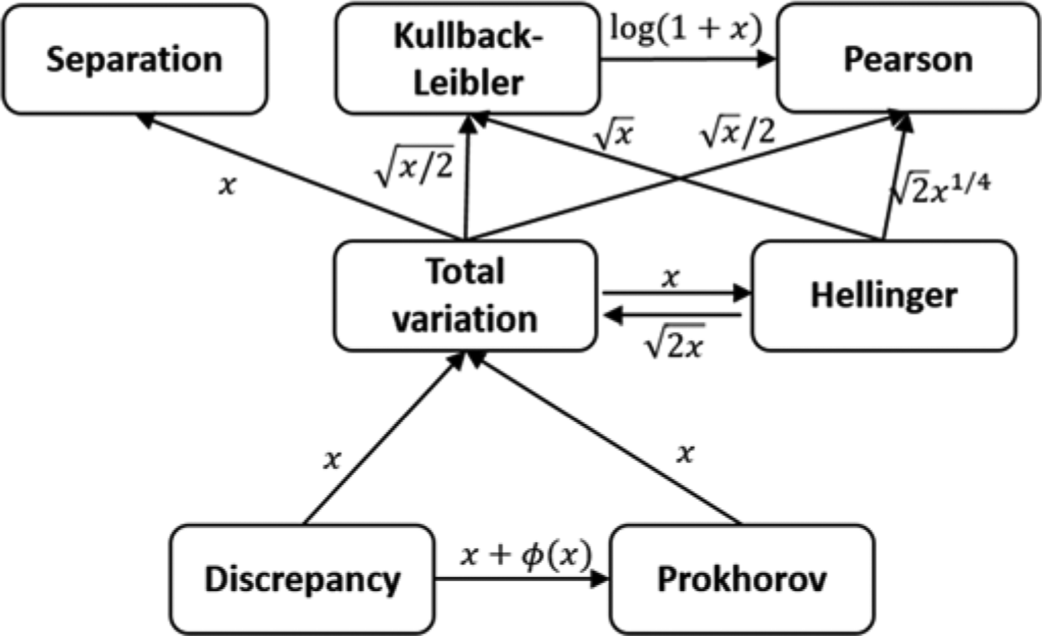
Relationships among probability metrics [39].
When detecting change points, one goal is to generate change point scores that are maximally sensitive to subtle changes in the data, because this will offer the greatest potential to identify both subtle and dramatic changes in the time series. In terms of difference values, this sensitivity results in a larger range of difference values. Because the metrics that appear at the end of a chain in Figure 2 have the largest value, we hypothesize that metrics at the top of the graph such as Kullback-Leibler divergence, Pearson divergence, and Separation distance are preferable for CPD algorithms. This hypothesis is supported by a study comparing uLSIF and KLIEP change point detection algorithms. Liu et al. [11] showed that both uLSIF and RuLSIF (using the Pearson metric) outperformed KLIEP (using the Kullback-Leibler metric). Sugiyama [40] also showed that the Pearson divergence has higher numerical stability and is more robust against outliers than Kullback-Leibler divergence. These are the only metrics in Figure 2 that have been utilized to date in CPD algorithms.
Another metric that provides a large difference is the Separation distance metric (S). While the graph in Figure 2 indicates that Separation distance has a greater value range than Total Variation distance (TV), information is not available about its relationship with the Pearson (PE) or Kullback-Leibler (KL) metrics. Furthermore, it has nott been investigated for use as a sensitive CPD measure. One of the unique contributions of this work is to use the Separation distance metric to develop a new density ratio-based change point detection algorithm. To the best of our knowledge there is not any change point detection algorithm using this metric. We also further complete Figure 2 by adding edges that relate Separation distance to other known metrics.
We start by deriving the metric for our SEParation distance CPD algorithm, called SEP. As with the previous methods, we compare the probability densities of ft(x) and ft−1(x) corresponding to two consecutive windows in the time series data, each with length n. We model the density ratio between these probability densities without estimating the densities ft(x) and ft−1(x) using Equation 10.
| (10) |
The parameters θ in the model g will be determined from data samples and K is a non-negative basis function. One appropriate basis function choice is Kernel functions. We determine the parameters θ in the model such that the difference between the actual and estimated ratios is minimized, as shown in Equation 11.
| (11) |
Since the first term in Equation 11 is constant in each window and does not relate to the estimated ratio, we will remove it from the minimization process and only use the second term. By substituting gt(x) in Equation 11 with the model from Equation 10, we can generate the optimization problem as shown in Equation 12.
| (12) |
Approximating the integrals using empirical averages, we obtain Equation 13.
| (13) |
where is the n-dimensional vector given by Equation 14.
| (14) |
Next, we will add the penalty term for the purpose of regularization and convergence and generate the optimization problem shown in Equation 15. Here, λ≥0 denotes the regularization parameter, which is chosen empirically by cross-validation [11].
| (15) |
When solving the optimization by setting the first-order differential to zero, parameter θ can be analytically obtained as shown in Equation 16.
| (16) |
Given a density-ratio estimator g(x), an approximator of the SEP change point score can finally be constructed as shown in Equation 17.
| (17) |
Similar to RuLSIF and ulSIF method, SEP change detection offers an analytical solution and is stable. We can then use SEP scores to detect change points. Considering the fact that a greater SEP score means that the probability of a change point is greater, as with the other methods in this category we reject all candidate points whose SEP values are lower than a threshold value. To reduce the chance of false alarms and avoid double change points, we only consider the peak score value as a change point. The threshold value (Th) will be chosen based on optimal performance for a particular time series. In our experiments, we identify a threshold value that optimizes a tradeoff between TPR and FPR for a subset of the data. Another important parameter in the SEP algorithm is the length of window (n). As with the threshold value, we vary the window size for each dataset in order to find the best window length in terms of both acceptable accuracy and real-time detection.
In the next step, we need to compare the SEP score approximation from Equation 17 to the Pearson score approximation in Equation 8. To find the relation between SEP and PE, we can rewrite Equation 8 as Equation 18.
| (18) |
Assuming function g in both equations represents the ratio between probability densities, we can substitute Equation 18 into Equation 17, yielding Equation 19.
| (19) |
Considering the third term on the right hand side as a new parameter k, we can rewrite the relation as given in Equation 20.
| (20) |
Since k is non-positive, from Equation 20 we know that the SEP score is always greater than or equal to the PE score. Thus, we can complete the relationship for metric S in Figure 2, yielding the graph shown in Figure 3. Based on our earlier claim that metrics at the end of the chain provide the most useful metrics for CPD algorithms, we hypothesize that change point detection using Separation distance (S) will generally outperform Pearson divergence for change point detection. Because the arrow from TV to S is annotated with a function that is asymptotically larger than the function annotating the arrow from TV to KL, we postulate that S will also generally outperform Kullback-Leibler divergence for change point detection as well.
Fig. 3.

Relationships among Separation and Pearson metrics.
4. Results And Discussion
In this section, we evaluate our proposed SEP change point detection and compare results with other popular CPD methods. First, we introduce performance measures that are used to evaluate aspects of the CPD process. Next, we summarize results for artificial and real-world datasets including smart home activity data, ECG data, and hand outline data.
4.1. Performance Measures
A number of measures are commonly used to evaluate the performance of change point detection methods. We use four different performance measures to evaluate the ability of our proposed SEP change point detection algorithm to detect both change points and non-change points in time series.
Sensitivity, also referred to as Recall or the True Positive Rate (TP Rate).
This refers to the portion of a class of interest (in this case, change points) that was recognized correctly. Here TP denotes the number of change points that were correctly detected and FN denotes the number of change points that were not detected. This measure provides an indication of how effectively a CPD algorithm will detect true state changes.
| (21) |
False Positive Rate (FP Rate).
This refers to the ratio of negative examples (in this case, the number of data points in a time series which are not change points) which are recognized as change points to the total number of negative examples. Here FP denotes the number of non-change points that were incorrectly identified as change points and TN denotes the number of non-change points that were not labeled as change points. This measure reflects how many false alarms would be generated by a CPD algorithm.
| (22) |
G-mean.
A supervised learning algorithm that attempts to perform change point detection typically faces an imbalanced class distribution because the ratio of changes to total data is usually small. As a result, G-mean is commonly used as an indicator of CPD performance. This utilizes both Sensitivity and Specificity measures to assess the performance of the algorithm in terms of the ratio of positive accuracy (Sensitivity) and the ratio of negative accuracy (Specificity).
| (23) |
Detection Delay.
This directly measures how close the time value of each correctly-predicted CP is to the actual CP time value in the series. The absolute value of the time difference between the true predicted and actual CP time points is summed and normalized over the total number of change points.
| (24) |
Following the strategy found in previous research [7][11], we assume a detected change point is correct if there exists a change point in the data that occurs soon before or after the detected change point. In other words, a detected change point at time t* is correct if a true change point occurs in the time interval [t* − λ, t* + λ]. In our experiments, we consider λ=1 second for the evaluation of exact change point detection and λ=5 and 10 seconds for evaluation of change point detection with a small time off-set.
4.2. Artificial Dataset
We use the following three artificial time-series datasets [11] that contain manually inserted change points to show the effectiveness of SEP method in detecting different changes and compare the performance to existing similar methods.
Dataset 1(Jumping mean).
The following 1-dimensional auto-regressive model is used to generate 1000 samples:
| (25) |
where єt is Gaussian noise with mean μ and standard deviation 0.5. The initial values are set as y(1) = y(2) = 0. A change point is inserted at every 100 time steps by increasing the noise mean μ by 2.
Dataset 2 (Scaling variance).
The same auto-regressive model as Dataset 1 is used, but a change point is inserted at every 100 time steps by infusing origin-centered noise with a random standard deviation between 0.01 and 1.
Dataset 3 (Changing frequency).
1-dimensional samples of size 1000 are generated as:
| (26) |
Where єt is origin-centered Gaussian noise with standard deviation 0.8. A change point is inserted at every 100 points by multiplying the frequency ω by 5.
To investigate the sensitivity of SEP performance on different choices of window size (n) and threshold value (Th), we calculate G-mean values because these reflect the ability of the algorithm to detect both change and non-change points. Figures 4 through 6 show the sensitivity analysis of SEP using the artificial datasets for exact, within-5-seconds and within-10-seconds CPD. For each case, the top figure shows the 3d plot of G-mean values for different threshold and window length values and the bottom figure shows the corresponding filled contour plot. The color bar demonstrates the value range of each color. As we can see from the graphs, by increasing the acceptable delay value the overall performance will improve for all datasets. We observe an almost flawless performance of SEP with no delay for the Jumping Mean and Scaling Variance datasets. In the case of the Changing Frequency dataset some detection delay is observed. Based on the results of this sensitivity analysis, the selected window lengths for Datasets 1, 2, and 3 are 30, 20, and 20, respectively. The threshold values are selected as 0.5 for Datasets 1 and 2 and 0.2 of the maximum score for Dataset 3.
Fig. 4.
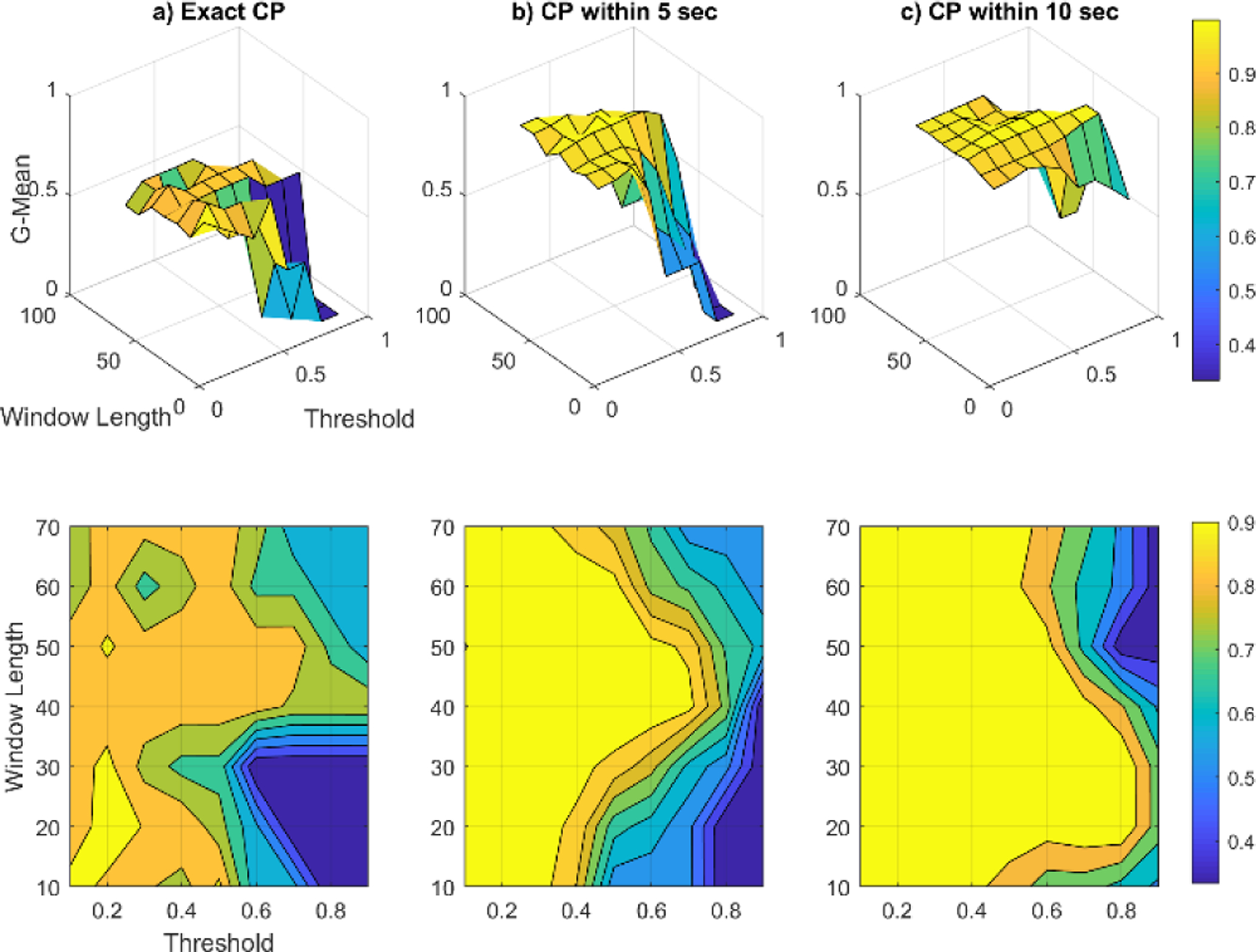
SEP algorithm sensitivity analysis for artificial dataset 1, Jumping Mean. The top row of graphs contains the 3d plots of G-mean values and the bottom row contains the corresponding contour plots.
Fig. 6.
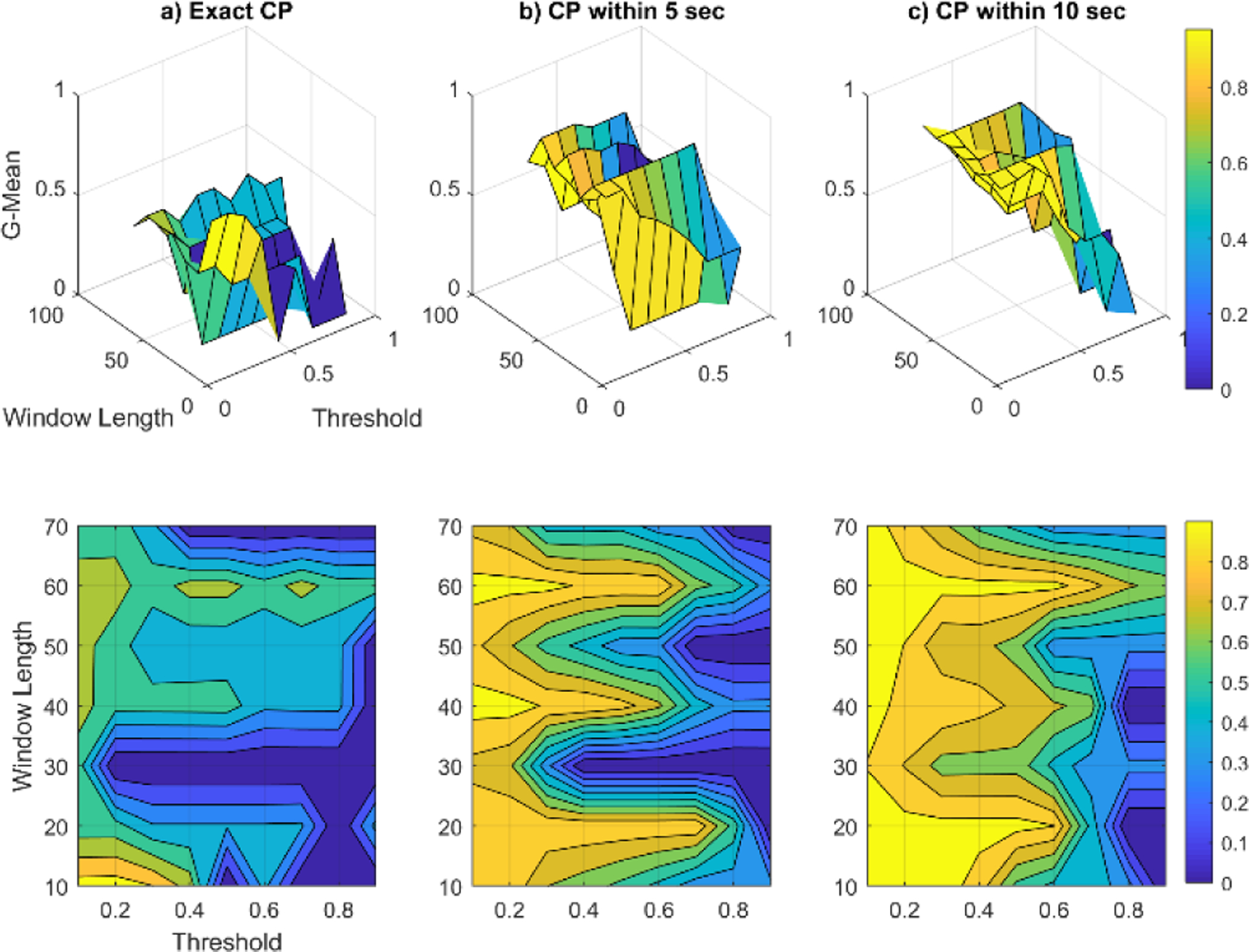
SEP algorithm sensitivity analysis for artificial dataset 3, Changing Frequency. The top row of graphs contains the 3d plots of G-mean values and the bottom row contains the corresponding contour plots.
Figures 7–9 visualize examples of these datasets as well as the corresponding change point score obtained by SEP, RuLSIF, and uLSIF. When there is a change in mean value, the change-point score obtained by all methods increases rapidly, but the value of the score is different for each method. The RuLSIF algorithm generates the same value regardless of the degree of change in the mean. In contrast, the SEP change score is more sensitive to these changes. For example, the largest SEP score occurs at time 900 where the mean increases from 10 to 50 while the smallest score occurs at time 100, 200, and 700 where the mean increases only 5. But RuLSIF score is constant for all of these changes. When the data variance changes, both SEP and RuLSIF catch these changes in addition to capturing false positive changes. When the data frequency changes, all CPD methods increase the change scores because the mean is also changing. As Figure 9 shows, SEP can generative the smallest number of false positive change points. In summary, SEP is more robust than the other methods against noise and outliers. We can see when there is no change and the data contains noise, the SEP score changes minimallywhile RuLSIF and uLSIF exhibit much larger change in their scores. This reflects the sensitivity of RuLSIF and uLSIF to noise and thus the change points are not consistently detected. On the other hand, the SEP method detects the existence of true change points in these complex situations.
Fig. 7.
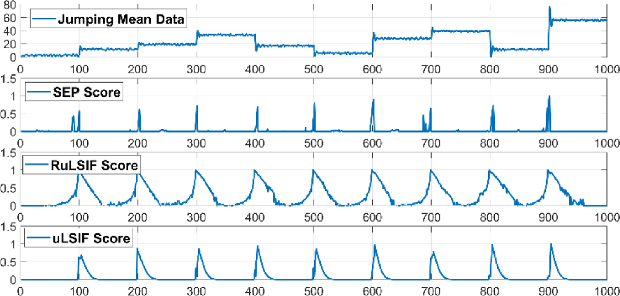
Jumping mean time-series samples and the change-point score obtained by different methods.
Fig. 9.
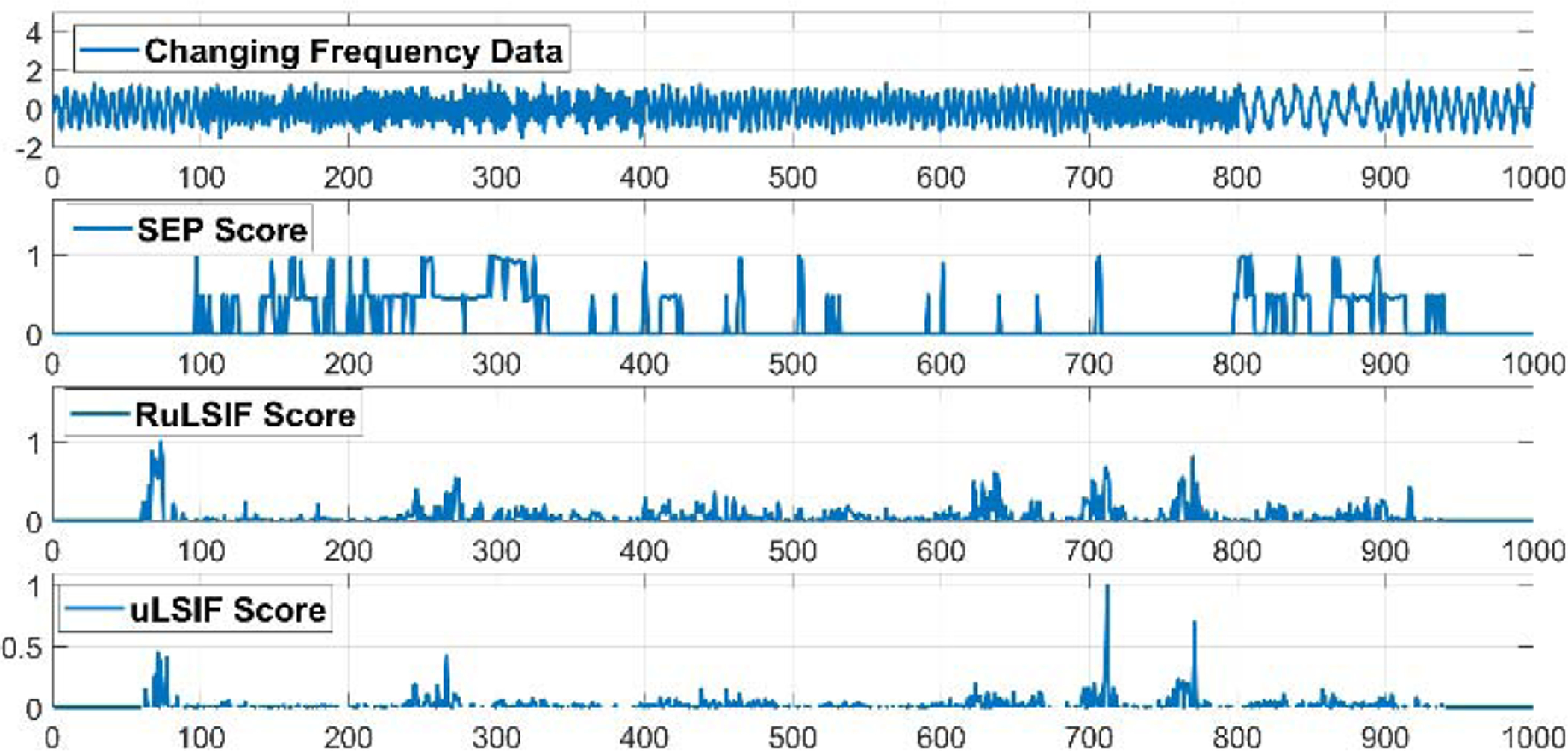
Changing frequency time-series samples and the change-point score obtained by different methods.
Next, we compare the performance of SEP with both RuLSIF and uLSIF in detecting within-10-seconds CPs using the TPR, FPR and G-mean measures. We also compare these methods with a simple baseline change detection. The baseline method performs a t-test comparison between two windows and reports a CP if the change in data is significant (p<.05). Table 2 summarizes these results. The window length for uLSIF and RuLSIF algorithm was set to 30, 20, and 60 for Datasets 1, 2, and 3, respectively, based on the highest performance we can achieve for this method. For the t-test these values are 40, 70, and 70 for each dataset because these values generated the best results for this baseline method.
TABLE 2.
Performance of CPD algorithm for artificial datasets.
| Dataset 1 - Jumping Mean | ||||
|---|---|---|---|---|
| SEP | RuLSIF | uLSIF | T test | |
| TPR | 1.00 | 1.00 | 0.56 | 1.00 |
| FPR | 0.03 | 0.05 | 0.01 | 0.14 |
| G-mean | 0.99 | 0.98 | 0.74 | 0.93 |
| Dataset 2 - Scaling Variance | ||||
| SEP | RuLSIF | uLSIF | T test | |
| TPR | 1.00 | 1.00 | 1.00 | 0.11 |
| FPR | 0.14 | 0.14 | 0.15 | 0.01 |
| G-mean | 0.93 | 0.93 | 0.92 | 0.33 |
| Dataset 3 - Changing Frequency | ||||
| SEP | RuLSIF | uLSIF | T test | |
| TPR | 1.00 | 1.00 | 0.44 | 0.22 |
| FPR | 0.13 | 0.25 | 0.01 | 0.06 |
| G-mean | 0.93 | 0.87 | 0.66 | 0.46 |
The results show, in the case of the Jumping Mean dataset, the SEP, RuLSIF, and t-test methods successfully detect all change points although SEP and RuLSIF reduce the false alarms in comparison to a basic t-test. However, there is not a significant difference in performance between SEP and RuLSIF. uLSIF algorithm exhibits the lowest FPR but since the TPR is not high we can conclude the small FPR value is because of its corresponding low detection rate. When there is a change in the variance of the data, the SEP and RuLSIF change point detection algorithms are significantly better than a basic t-test in detecting change points, but the uLSIF algorithm does not even outperform the baseline. Although there is not a significant difference between RuLSIF and SEP, SEP performs slightly better in detecting non-change points. For the Changing Frequency dataset, although SEP and RuLSIF again perform significantly better than a basic t-test and both of them detect all change points, SEP is significantly better than RuLSIF in detecting non-change points (the FPR value is almost half that of RuLSIF). In summary, we conclude that the SEP change point detection algorithm can detect changes in the mean, variance, and frequency of time series data. Furthermore, when detecting frequency changes SEP significantly outperforms the current state-of-the-art CPD algorithms. In addition, SEP can detect changes in frequency much faster than RuLSIF because of its smaller window length.
4.3. Smart Home Activity Transition Detection
Next, we apply the proposed change-point detection method to the real-world data. For this task, we select the CASAS smart home dataset [41]. This experiment allows us to validate our SEP algorithm on unscripted activity-labeled smart home data to determine if it can detect changes between activity states. Detecting transitions between activities in real time is useful for many applications. First, transition detection can be used to segment smart home sensor data into non-overlapping activity sequences and provide insights on the start time, stop time, and duration of activities performed in the home [42]. This segmentation can also boost the performance of activity recognition because the feature vector does not contain information from more than one activity and can include features such as activity start time and duration so far. Second, detection of activity transitions facilitates activity-aware delivery of notifications, automation and behavioral intervention technologies. Receiving notifications at inopportune times is not only annoying, but can increase a resident’s cognitive load [43], introduce task errors [44], and reduce acceptance of the technology [45]. Timing prompts and notifications during activity transitions can improve user response rates and support independent living [46].
4.3.1. CASAS Smart Home
The data used during this research was collected by the CASAS (Center for Advanced Studies in Adaptive Systems) smart home system [41] [47] developed at Washington State University. Using embedded sensors, the CASAS smart homes collect information about the state of the home and the resident(s) to monitor and analyze daily activities. Sensors generate “events” to report their state. An event contains a date, time, sensor identifier, and message sent from the sensor.
Each of the CASAS smart homes has at least one bedroom, a kitchen, a dining area, a living area, and at least one bathroom. All of the CASAS smart homes have different sizes and layouts, yet they all include the standard sensor setup. Each of the smart apartments is equipped with a network of wireless motion and door sensors and houses a single older adult resident who performs normal daily routines. Figure 10 shows the layout of one of the smart homes we analyze in this paper. Sensor labels starting with “M” indicate motion sensors and “D” indicates door sensors.
Fig. 10.
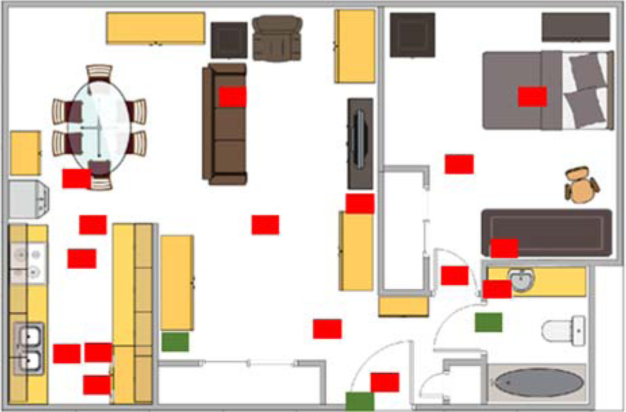
Smart home floorplan and positions of motion/light sensors (red) and door/temperature sensors (green).
The primary sensor found in CASAS smart homes is an overhead motion sensor. The motion sensors are used to determine when motion is occurring in the area covered by the sensor. The motion sensor reports an ON message when motion is detected, followed by an OFF message when the movement stops. In cases when the resident is walking under the motion sensor to some other location, the motion sensor has a gap between the ON and OFF messages that is roughly 1.25 seconds. However, if the activity results in continuous movement under the motion sensor, (e.g., dancing near the motion sensor), the sensor will not generate an OFF message until 1.25 seconds after the activity has stopped.
There are two types of motion sensors configurations utilized in the CASAS smart home system. The most common motion sensors used are the narrow-field motion sensors. In the case of narrow-field motion sensors, the sensor’s field of view is limited to a radius of a few feet. These sensors are placed on the ceiling of the home and detect movement within the sensor’s field of view. The other motion sensor configuration that is used throughout the smart home system is the wide-field motion sensor; the wide-field motion sensor has a much larger field of view. These area sensors are usually placed on the walls to determine whether there has been movement anywhere in an entire room. The wide-field motion sensor can only detect motion in the room, not localize where the resident is located inside the room. In contrast, the narrow-field motion sensors provides a finer-resolution localization of the resident.
Another sensor used in the CASAS smart home system is the magnetic door sensor. Door sensors use a magnetic switch to determine whether the doors are opened or closed. These are usually mounted on the external doors of the smart home to indicate when the resident enters or leaves the home, though some door sensors are also placed in strategic locations such as doors to cabinets that hold medicine dispensers.
We evaluate our SEP algorithm using data collected over two months in smart home testbeds that were installed in six apartments [41]. Each of the apartments house a single older adult (age 75+) resident who performs a normal daily routine while sensors in the apartment generate and store events. To provide ground truth activity labels, annotators are given the house floor plan, the positions of the sensors, a resident-completed form indicating when and where they typically perform daily activities, and the sequence of sensor events. Multiple annotators are used to provide consistent labels and the inter-annotator agreement is κ=0.80. The activity classes that we use for our analyses are Bathe, Enter Home, Wash Dishes, Personal Hygiene, Relax, Work, Sleep, Leave Home, Cook, Bed Toilet Transition, Eat, and Other Activity. Because all events that do not fit into the 11 predefined activity classes are labeled as “Other Activity”, the activities are skewed toward this activity class. Activity transitions are time in the sensor event data sequence when the activity changes from one label to a different label. These represent the change points we want to detect using our CPD algorithms. Distribution of transitions between all activities in six apartments are described in supplementary material section.
4.3.2. CASAS Smart Home Activity Transition Detection
For detecting activity transitions, our time series data was created in the following manner using continuous sensor events collected from CASAS smart homes. We slide a window over the sensor data that looks at 30 events and extract a corresponding feature vector. These features include general information such as window time duration, event time, and the most dominant sensor in the window which is most frequent triggered sensor, number of occurrence of each sensor in current window, the time when each sensor last fired till the end of current window, etc. Thus, the feature vector dimension varies depending on home floorplans and sensor placements.
The feature space is then updated when a new event occurs to yield our time series data. The raw data we collect in smart homes together with the features we use to learn activity models from smart home data are summarized in Table 3. Figure 12 plots a subset of CASAS smart home features (5 out of the 51 features) which comprises our multi dimensional time series. This figure contains seven different activities which are separated by vertical black lines.
TABLE 3.
Raw smart Home data, features, and activity class descriptors.
| Domain | Number | Types of Features |
|---|---|---|
| Raw Sensor data | 3 sensor types | infrared motion (ON/OFF), magnetic door (OPEN/CLOSE), ambient light (continuous) |
| Timing features | 3 features | day of week, hour of day, seconds past midnight |
| Window features | 9 features | most recent sensor in window, first sensor in window, window duration, most frequent sensors from previous two windows, last sensor location in window, last motion sensor location in window, entropy-based data complexity of window, time elapsed since last sensor event in window |
| Sensor features (n sensors in home) | 2*n features | count of events for each sensor in window, elapsed time for each sensor since last event |
Fig. 12.
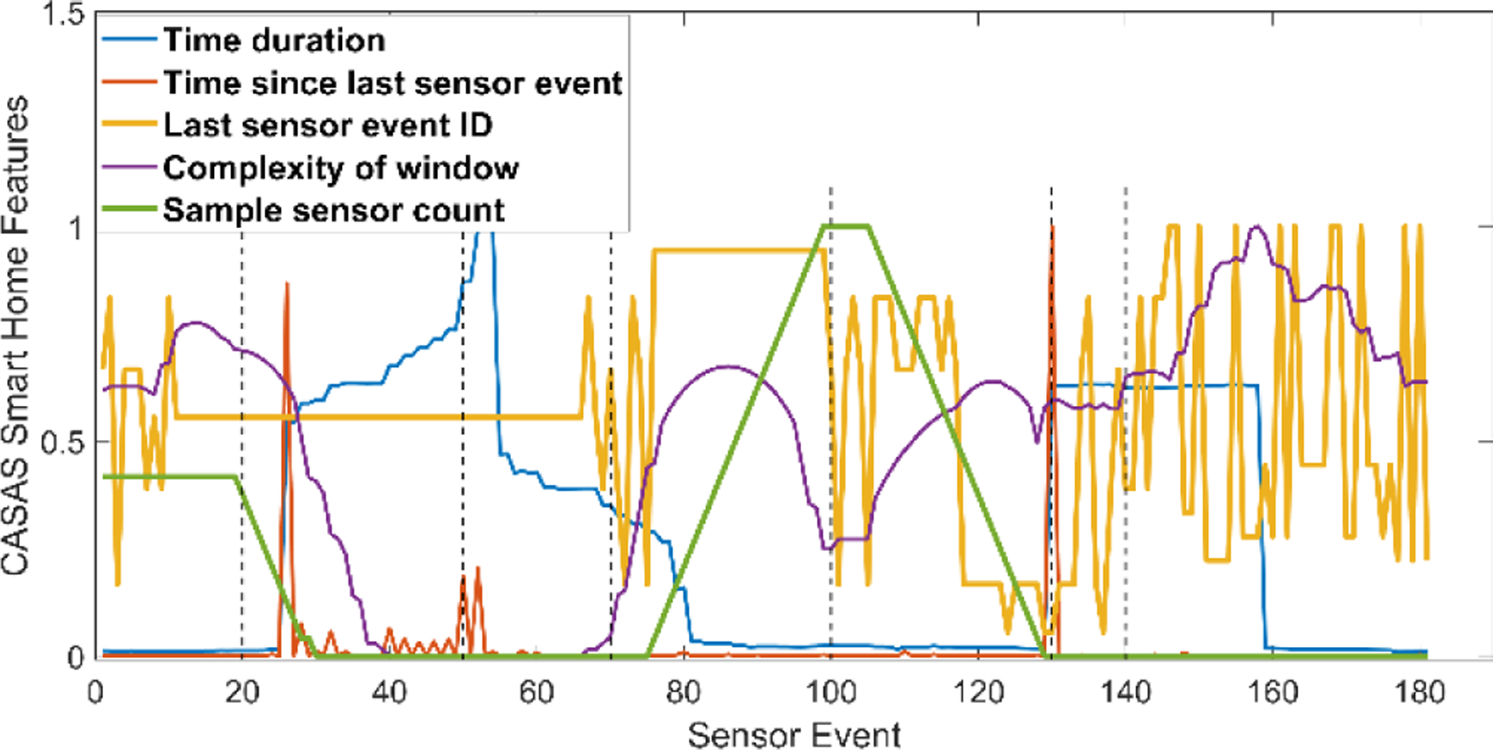
Sample CASAS smart home features. The true activity transitions are marked by black vertical lines.
For the smart home data, we again investigate the sensitivity of SEP’s G-Mean performance for different choices of window size (n) and threshold value (Th). We perform the sensitivity analysis for one of the CASAS homes over two months of data and then use the chosen parameters for the other smart home sites to show the generality of the model. Figure 13 shows the sensitivity analysis of SEP-based activity transition detection in Apartment 1 for exact, within 5 seconds, and within 10 seconds CP detection. As we can see from the graphs, by increasing the acceptable delay the overall performance improves and SEP can detect more transitions. There is not a significant difference in performance for a small window length (less than 20 sensor events) but increasing the window length can decrease the ability of SEP to find activity transitions. Based on the results of this preprocessing step, the selected value of n for all apartments was 2 sensor events which means our algorithm is 2-real time. Finally, the threshold value was set to 0.1.
Fig. 13.
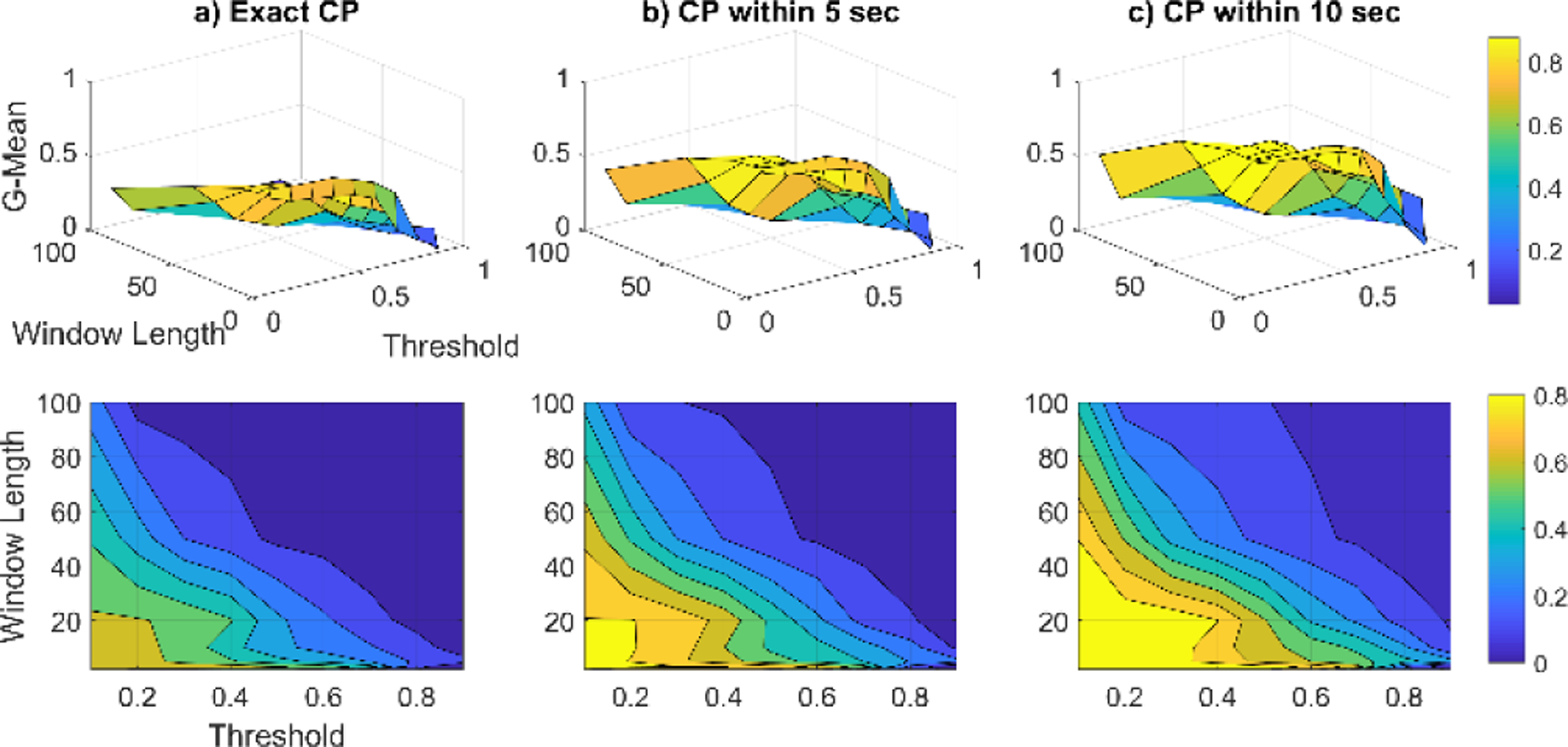
SEP algorithm sensitivity analysis for activity transition detection in Apartment 1. The top row of graphs contains the 3d plots of G-mean values and the bottom contains the corresponding contour plots.
Next, we compare the performance of SEP with two other density ratio based methods, RuLSIF and uLSIF [11]. Figure 14 plots the within-10-second change detection ROC curves for these methods over different threshold values for two of the apartments. The experimental results show that the ROC curves of all of these methods exhibit similar behavior when changing the threshold value. Overall, the SEP algorithm outperforms the other methods with the largest area under ROC curve (AUC) value. Since the experimental conditions are similar for the alternative CPD algorithms, we can conclude the difference is because of the SEP dissimilarity measure that we introduce. As Figure 14 indicates, the Separation distance is more successful than the Pearson measure in detecting activity transitions.
Fig. 14.
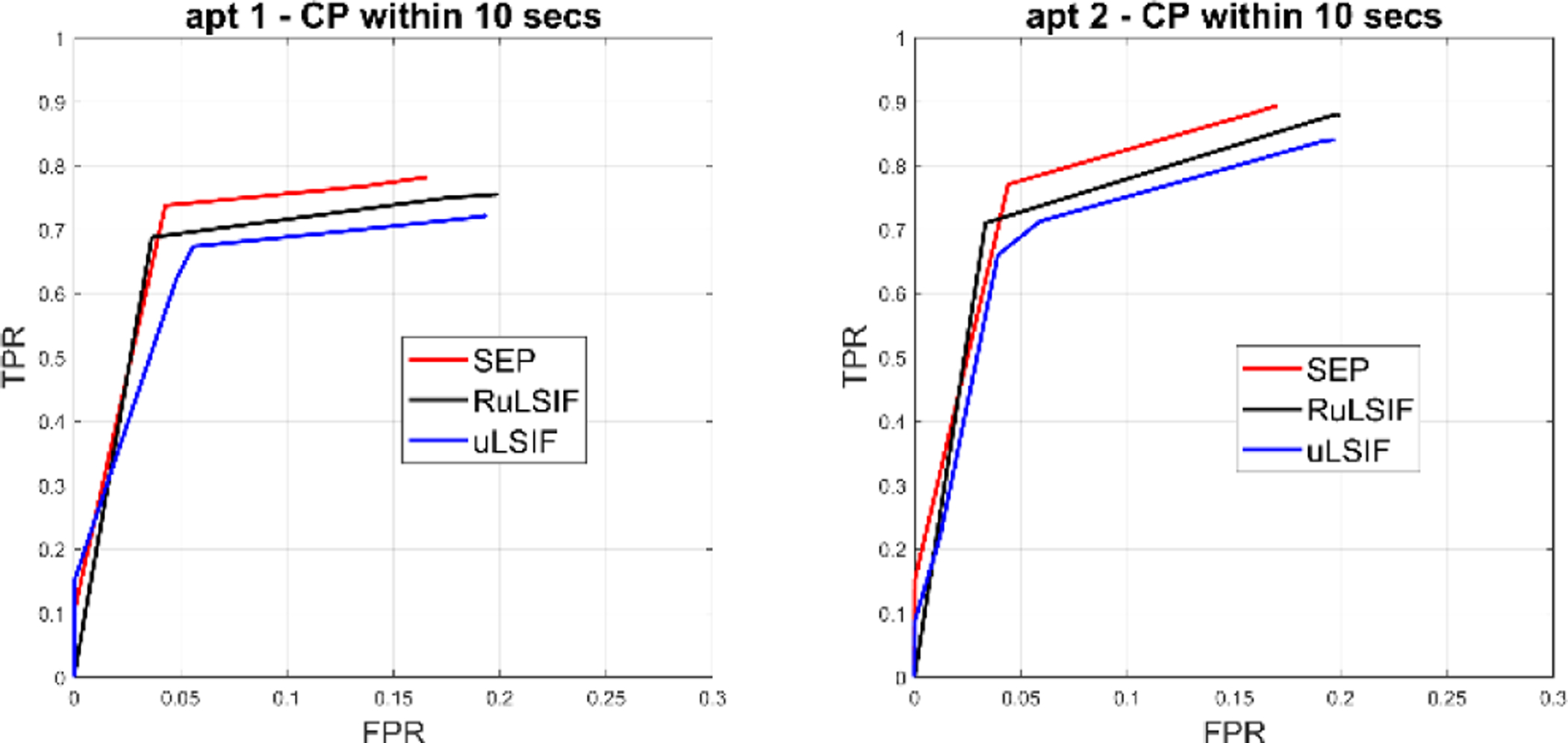
ROC curve and AUC values for activity transition detection based on two smart homes.
Figure 15 plots the sensitivity of the Detection Delay value to the threshold value for our selected direct density ratio CPD methods. When increasing the threshold value, there is a subsequent increase in both TPR and FPR. Additionally, the average distance between detected change points and the actual change point increases for all algorithms. However, as we can see in the figure SEP has the smallest Detection Delay value and lowest sensitivity to the threshold. This provides evidence not only that SEP can detect transitions closer to their actual occurrence, but also that changing the threshold value does not greatly affect this performance. Since all of these algorithms are 2-real time and as we demonstrated, SEP outperforms RuLSIF and uLSIF in terms of both AUC and Detection Delay, we can conclude that the SEP algorithm offers superior performance for detecting activity change points in real time.
Fig. 15.
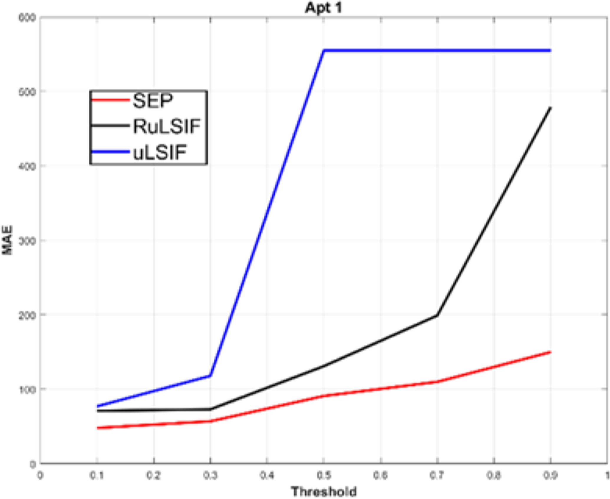
Detection Delay value for activity transition detection.
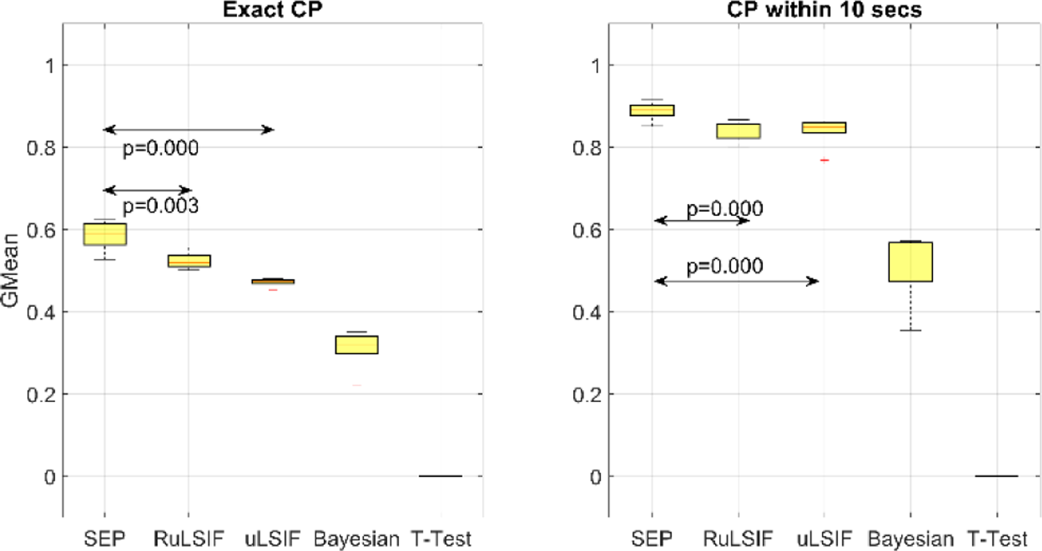
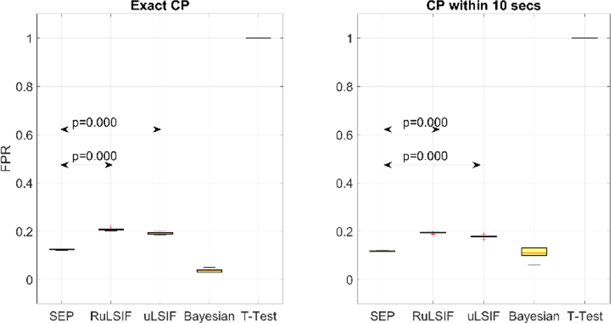
Figure 16 through Figure 18 show the TPR, FPR, and G-Mean values for the SEP, RuLSIF, uLSIF, Bayesian, and t-test methods [25] based on exact CP and CP within 10 seconds, respectively. The figures show that as expected, except for the t-test baseline, change point detection within 10 seconds exhibits better performance than exact change point detection. This is because all of the CPD algorithms experience a delay in detecting changes or transitions. SEP outperforms all other methods in detecting activity transitions with an average True Positive Rate = 0.89 for a within-10-seconds detection. As we can see in figure, the result indicates the difference is significant at the (p < .05) level.
Fig. 16.
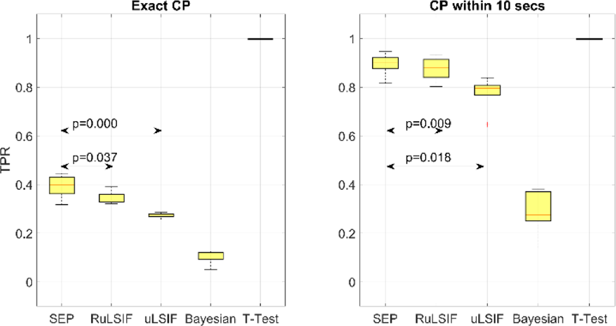
TPR scores for activity transition detection.
Fig. 18.
G-Mean scores for activity transition detection.
SEP algorithm has a lower False Positive Rate (average = 0.12) than RuLSIF and uLSIF, but its FPR is higher than the Bayesian algorithm. Recalling that the Bayesian CPD has a very low TPR and thus it cannot detect changes consistently, we conclude the small FPR value in this method is because of its overall low detection rate. This result is consistant with our previous finding that SEP is more robust against noise or outliers than the other methods. Because human behavior (and therefore smart home sensor data) is noisy, SEP performs better in this case and detects fewer false alarms. The one-way ANOVA test indicates the difference between FPR values for SEP and the other algorithms is significant at the (p < .05) level. The G-Mean results are similar to those for TPR and show in summary that SEP outperforms all other algorithms in detecting both transitions and non-transitions with an average of 0.88. The one-way ANOVA test indicates the difference between G-Mean performances is significant at the (p < .05) level. In summary, the baseline t-test experiment between two consecutive windows reveals that a simple t-test detects almost all windows as transitions, so both TPR and FPR values are 1 and the G-Mean is 0. This result indicates that using change point detection algorithms is necessary for detecting activity transitions. Although the Bayesian algorithm exhibits better performance than baseline, it is not a promising tool for detecting activity transitions. One possible explanation is that the nature of human behavior data is highly variable and thus is difficult to predict using purely Bayesian methods with relatively small amounts of data.
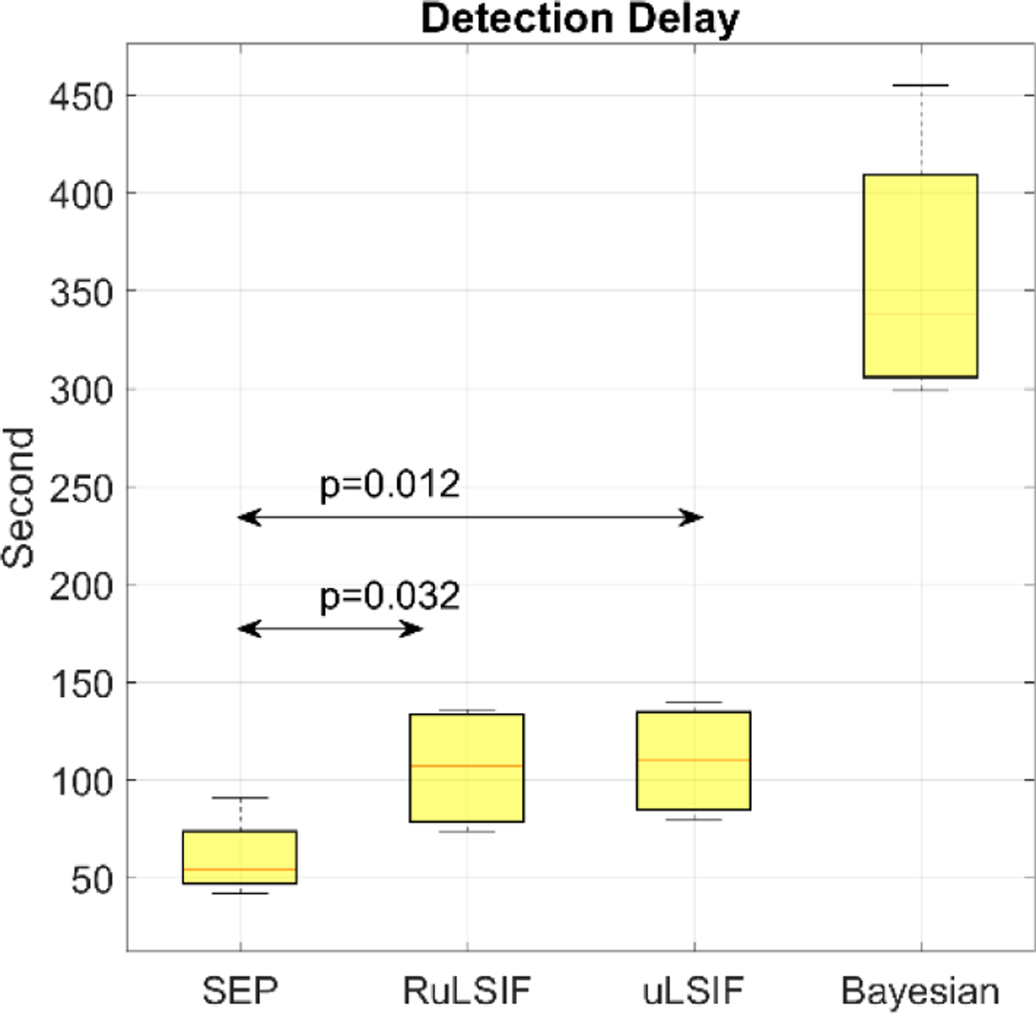
Finally, the Detection Delay for all algorithms is plotted in Figure 19. The Detection Delay can be thought of as the average time between when a transition occurs and when the transition is detected. For the SEP algorithm, the average value is close to 60.5 seconds, or 1.01 minutes, which is lower than all other methods. The delay values for the RuLSIF, uLSIF, and Bayesian methods are 1.76, 1.83, and 6.00 minutes, respectively. Ideally, we would like to minimize these times to have more accurate activity boundaries. By considering the length of activities in the real world (12 minutes is the average for our datasets), we determine all density ratio based methods have an acceptable Detection Delay for many automation and notification applications, but still have room for improved responsiveness. From the above results, we can see that the best performance for activity transition detection results from applying the SEP algorithm. The baseline t-test Detection Delay was not calculated due its poor performance based on FPR and G-mean measures.
Fig. 19.
Detection Delay scores for activity transition detection.
4.4. Other Real-World Datasets
To show the generality of SEP change point detection, we evaluate the performance of SEP and other existing change-point detection methods using two additional real-world datasets: ECG and hand outline. Both datasets are drawn from the UCR Time Series Data Mining Archive [48].
The ECG dataset is a respiration dataset which records patients’ respiration measured by thorax extension as they wake up. The series is manually segmented by a medical expert. Table 4 shows the results of ECG change point detection using the SEP, RuLSIF, and Bayesian algorithms. The results again show both SEP and RuLSIF yield superior performance to the Bayesian method. We can see SEP has a high FPR which can be because of the periodic nature of this time series. Thus, although it has a slightly better TPR than RulSIF, the G-Mean score is lower. In terms of the distance between actual and detected change points, SEP exhibits the lowest Detection Delay. The one-way ANOVA test indicates that the difference between alternative algorithm performances is not significant at the (p < .05) level. Performing a t-test to compare the performance of algorithms shows that SEP and RuLSIF have similar performances for this dataset but both of them have significantly better performances than uLSIF and the Bayesian method at the (p < .05) level.
TABLE 4.
ECG dataset result.
| SEP | RuLSIF | uLSIF | Bayesian | |
|---|---|---|---|---|
| TPR | 0.80 | 0.75 | 0.02 | 0.24 |
| FPR | 0.24 | 0.12 | 0.00 | 0.01 |
| G-Mean | 0.78 | 0.81 | 0.14 | 0.49 |
| Detection Delay | 13 | 55 | - | 87 |
Next, we apply the alternative CPD methods to the hand outline dataset. Table 5 shows the results for the SEP, RuLSIF, uLSIF, and Bayesian algorithms. Again, we can see from the results that SEP outperforms the other methods in terms of TPR, G-Mean, and Detection Delay, but still has a slightly higher FPR than the other approaches. The one-way ANOVA test indicates the difference between alternative algorithm TPR and G-mean value is significant at the (p < .05) level.
TABLE 5.
Hand outline dataset result.
| SEP | RuLSIF | uLSIF | Bayesian | |
|---|---|---|---|---|
| TPR | 0.72 | 0.50 | 0.04 | 0.02 |
| FPR | 0.14 | 0.03 | 0.00 | 0.00 |
| G-Mean | 0.79 | 0.70 | 0.21 | 0.15 |
| Detection Delay | 52 | 154 | - | 1227 |
In summary, the results show that our SEP change point detection method outperforms other methods for many time series datasets. The results also indicate that although the performance of change point detection algorithm is highly dependent upon the nature of the data set, the uLSIF and Bayesian algorithms are not useful for these types of real-world change point detection problems.
With respect to other direct density ratio methods (KLIEP, uLSIF, RuLSIF) as well as the well-known Bayesian method, these methods are also ε-real time, however, as we demonstrated, SEP outperforms them in terms of TPR, G-Mean, and Detection Delay, which provides evidence that the SEP algorithm can detect changes more accurately and with less detection delay.
With respect to other unsupervised CPD methods (including SWAB, CF, MDL, kernel-based, and graph-based approaches), SEP is preferable because it is nonparametric, closer to real time, and handles arbitrary dimensionality. In contrast, CF [32], CUSUM [31], SI [23], and SST [24] are parametric methods. Clustering change point detection methods such as SWAB [27], MDL [28], and Shapelet [29] are offline or near offline, and both kernel-based methods [30] and graph-based methods [15] can only handle independent and identically distributed (i.i.d.) time series.
5. Conclusion
In this paper, we formulate the problem of change point detection. Based on a review of existing change point detection methods and difference measures used in density ratio-based approaches, we hypothesized that metrics with larger range of difference value perform better for consistently detecting change points in complex data. In response, we introduce a change point algorithm based on Separation distance for real-time detection of change points. From the experimental validation of artificial and real-world datasets, we observe that the proposed algorithm outperforms existing methods such as smart home activity transition detection. However, the method does not always outperform other approaches, as observed in the case of the ECG dataset. Our proposed SEP algorithm hands high-dimensional data and detects change points in near-real time using most commonly a 2-data point look ahead. Although other density ratio based methods also address these situations, our experimental results show in many cases SEP demonstrates superior performance.
Although the proposed method was shown to work well in most cases, its performance may improve further by adding the effect of previous windows to the CP score calculation. We will experiment with these enhancements in future work. Additionally, the selection of a threshold value has a great impact on the performance of density ratio-based change point detection algorithms. In this work we used constant increments when we were testing threshold values. Using other methods like gradient descent or a Gaussian approach may result in a more optimal threshold value. Another limitation of SEP and all of density ratio change point detection methods is their computational cost. One important direction for future work is to improve the computational efficiency of this algorithm. Decreasing computational cost will aid our integration of the SEP algorithm into real-world applications such as activity segmentation and delivery of behavioral interventions. We can then elicit user feedback on the appropriate determination of change points and their use in interventions.
Fig. 5.
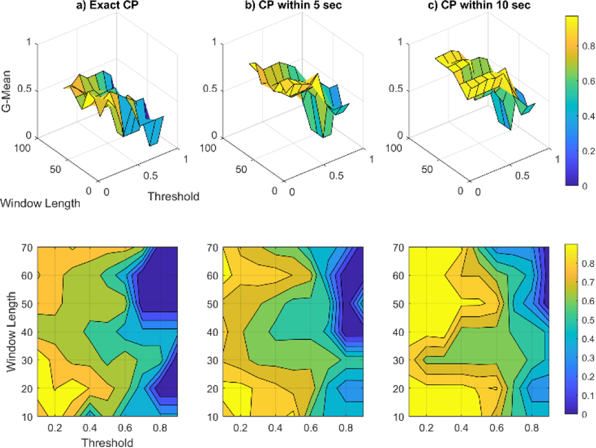
SEP algorithm sensitivity analysis for artificial dataset 2, Scaling Variance. The top row of graphs contains the 3d plots of G-mean values and the bottom row contains the corresponding contour plots.
Fig. 8.
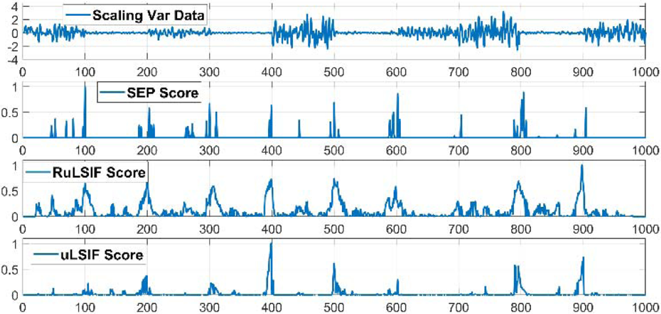
Scaling variance time-series samples and the change-point score obtained by different methods.
Fig. 17.
FPR scores for activity transition detection.
Acknowledgment
This research has been supported in part by National Science Foundation grant 1543656 and National Institutes of Health grant R01EB009675.
Biography

Samaneh Aminikhanghahi is currently a Ph.D. candidate in computer science at Washington State University. She received her B.S. in electrical engineering (1999), M.S in electrical engineering (2003) and M.S. in computer science (2014). Her research interests include machine learning, smart environments, and automated health intervention.

Tinghui Wang was born in China in 1988. He received the B.E. degree in Microelectronics from Shanghai Jiaotong University, Shanghai, China, 2009. He joined Digilent Inc, China Office and Beecube Inc, China Office after graduation. He is currently pursuing the Ph.D. in electrical engineering at Washington State University. His current research involves activity recognition, multi-target tracking in smart home environments with binary sensors.

Diane J. Cook is a Huie-Rogers Chair Professor at Washington State University. She received her Ph.D. in computer science from the University of Illinois and her research interests include machine learning, pervasive computing, and designed of automated strategies for health monitoring and intervention. She is an IEEE Fellow and a Fellow of the National Academy of Inventors.
References
- [1].Malladi R, Kalamangalam GP, and Aazhang B, “Online Bayesian change point detection algorithms for segmentation of epileptic activity,” in Asilomar Conference on Signals, Systems and Computers, 2013, pp. 1833–1837. [Google Scholar]
- [2].Reeves J, Chen J, Wang XL, Lund R, and Lu QQ, “A Review and Comparison of Changepoint Detection Techniques for Climate Data,” J. Appl. Meteorol. Climatol, vol. 46, no. 6, pp. 900–915, Jun. 2007. [Google Scholar]
- [3].Itoh N and Kurths J, “Change-Point Detection of Climate Time Series by Nonparametric Method,” in World Congress on Engineering and Computer Science 2010 Vol I, 2010. [Google Scholar]
- [4].Chowdhury MFR, Selouani S-A, and O’Shaughnessy D, “Bayesian on-line spectral change point detection: a soft computing approach for on-line ASR,” Int. J. Speech Technol, vol. 15, no. 1, pp. 5–23, Oct. 2011. [Google Scholar]
- [5].Rybach D, Gollan C, Schluter R, and Ney H, “Audio segmentation for speech recognition using segment features,” in IEEE International Conference on Acoustics, Speech and Signal Processing, 2009, pp. 4197–4200. [Google Scholar]
- [6].Radke RJ, Andra S, Al-Kofahi O, and Roysam B, “Image change detection algorithms: a systematic survey,” IEEE Trans. Image Process, vol. 14, no. 3, pp. 294–307, Mar. 2005. [DOI] [PubMed] [Google Scholar]
- [7].Feuz KD, Cook DJ, Rosasco C, Robertson K, and Schmitter-Edgecombe M, “Automated Detection of Activity Transitions for Prompting,” IEEE Trans. Human-Machine Syst, vol. 45, no. 5, pp. 1–11, 2014. [DOI] [PMC free article] [PubMed] [Google Scholar]
- [8].Rawassizadeh R, Momeni E, Dobbins C, Gharibshah J, and Pazzani M, “Scalable Daily Human Behavioral Pattern Mining from Multivariate Temporal Data,” IEEE Trans. Knowl. Data Eng, vol. 28, no. 11, pp. 3098–3112, Nov. 2016. [Google Scholar]
- [9].Reyes-Ortiz J-L, Oneto L, Samà A, Parra X, and Anguita D, “Transition-Aware Human Activity Recognition Using Smartphones,” Neurocomputing, vol. 171, pp. 754–767, Jan. 2016. [Google Scholar]
- [10].Downey AB, “A novel changepoint detection algorithm,” Dec. 2008.
- [11].Liu S, Yamada M, Collier N, and Sugiyama M, “Change-point detection in time-series data by relative density-ratio estimation.,” Neural Netw, vol. 43, pp. 72–83, Jul. 2013. [DOI] [PubMed] [Google Scholar]
- [12].Sprint G, Cook DJ, Fritz R, and Schmitter-Edgecombe M, “Using Smart Homes to Detect and Analyze Health Events,” Computer, vol. 49, no. 11, pp. 29–37, Nov. 2016. [Google Scholar]
- [13].Ni Q, García Hernando AB, and de la Cruz IP, “The Elderly’s Independent Living in Smart Homes: A Characterization of Activities and Sensing Infrastructure Survey to Facilitate Services Development.,” Sensors, vol. 15, no. 5, pp. 11312–62, May 2015. [DOI] [PMC free article] [PubMed] [Google Scholar]
- [14].Tran D-H, “Automated Change Detection and Reactive Clustering in Multivariate Streaming Data,” Nov. 2013.
- [15].Chen H and Zhang N, “Graph-Based Change-Point Detection,” Ann. Stat, vol. 43, no. 1, pp. 139–176, Sep. 2014. [Google Scholar]
- [16].Harchaoui Z, Moulines E, and Bach FR, “Kernel Change-point Analysis,” in Advances in Neural Information Processing Systems, 2009, pp. 609–616. [Google Scholar]
- [17].Cleland I et al. , “Evaluation of prompted annotation of activity data recorded from a smart phone.,” Sensors (Basel)., vol. 14, no. 9, pp. 15861–79, Jan. 2014. [DOI] [PMC free article] [PubMed] [Google Scholar]
- [18].Han M, Vinh LT, Lee Y-K, and Lee S, “Comprehensive Context Recognizer Based on Multimodal Sensors in a Smartphone,” Sensors, vol. 12, no. 12, pp. 12588–12605, Sep. 2012. [Google Scholar]
- [19].Zheng Y, Chen Y, Xie X, and Ma W-Y, “Understanding transportation modes based on GPS data for Web applications - Microsoft Research,” ACM Trans. Web, vol. 4, no. 1, 2010. [Google Scholar]
- [20].Cook DJ and Krishnan NC, Activity Learning: Discovering, Recognizing, and Predicting Human Behavior from Sensor Data. Wiley, 2015. [Google Scholar]
- [21].Desobry F, Davy M, and Doncarli C, “An online kernel change detection algorithm,” IEEE Trans. Signal Process, vol. 53, no. 8, pp. 2961–2974, Aug. 2005. [Google Scholar]
- [22].Hido S, Idé T, Kashima H, Kubo H, and Matsuzawa H, “Unsupervised Change Analysis using Supervised Learning,” Adv. Knowl. Discov. Data Min, vol. 5012, pp. 148–159, 2008. [Google Scholar]
- [23].Kawahara Y, Yairi T, and Machida K, “Change-Point Detection in Time-Series Data Based on Subspace Identification,” in 7th IEEE ICDM 2007, pp. 559–564. [Google Scholar]
- [24].Moskvina V and Zhigljavsky A, “An Algorithm Based on Singular Spectrum Analysis for Change-Point Detection,” Commun. Stat. - Simul. Comput, vol. 32, no. 2, pp. 319–352, Jan. 2003. [Google Scholar]
- [25].Adams RP and MacKay DJC, “Bayesian Online Changepoint Detection,” Machine Learning, Oct. 2007. [Google Scholar]
- [26].Saatçi Y, Turner RD, and Rasmussen CE, “Gaussian Process Change Point Models,” in International Conference on Machine Learning, 2010, pp. 927–934. [Google Scholar]
- [27].Keogh E, Chu S, Hart D, and Pazzani M, “An online algorithm for segmenting time series,” in IEEE International Conference on Data Mining, 2001, pp. 289–296. [Google Scholar]
- [28].Rakthanmanon T, Keogh EJ, Lonardi S, and Evans S, “MDL-based time series clustering,” Knowl. Inf. Syst, vol. 33, no. 2, pp. 371–399, Nov. 2012. [Google Scholar]
- [29].Zakaria J, Mueen A, and Keogh E, “Clustering Time Series Using Unsupervised-Shapelets,” in IEEE 12th International Conference on Data Mining, 2012, pp. 785–794. [Google Scholar]
- [30].Harchaoui Z, Vallet F, Lung-Yut-Fong A, and Cappe O, “A regularized kernel-based approach to unsupervised audio segmentation,” in IEEE International Conference on Acoustics, Speech and Signal Processing, 2009, pp. 1665–1668. [Google Scholar]
- [31].Basseville M and Nikiforov IV, Detection of Abrupt Changes-theory and application. Prentice Hall, 1993. [Google Scholar]
- [32].Yamanishi K and Takeuchi J, “A unifying framework for detecting outliers and change points from non-stationary time series data,” in 8th ACM SIGKDD international conference on Knowledge discovery and data mining - KDD ‘02, 2002, p. 676. [Google Scholar]
- [33].Kawahara Y and Sugiyama M, “Sequential Change-Point Detection Based on Direct Density-Ratio Estimation,” in SIAM International Conference on Data Mining, 2009, pp. 389–400. [Google Scholar]
- [34].Zhang X, “Machine learning and big data analytics for the smart grid,” Georgia Institute of Technology, 2017. [Google Scholar]
- [35].Sugiyama M, Suzuki T, Nakajima S, Kashima H, von Bünau P, and Kawanabe M, “Direct importance estimation for covariate shift adaptation,” Ann. Inst. Stat. Math, vol. 60, no. 4, pp. 699–746, Dec. 2008. [Google Scholar]
- [36].Kanamori T, Hido S, and Sugiyama M, “A Least-squares Approach to Direct Importance Estimation,” J. Mach. Learn. Res, vol. 10, pp. 1391–1445, 2009. [Google Scholar]
- [37].Yamada M, Kimura A, Naya F, and Sawada H, “Change-point detection with feature selection in high-dimensional time-series data,” in International Joint Conference on AI, 2013. [Google Scholar]
- [38].Sugiyama M et al. , “Direct Divergence Approximation between Probability Distributions and Its Applications in Machine Learning,” J. Comput. Sci. Eng, vol. 7, no. 2, pp. 99–111, 2013. [Google Scholar]
- [39].Gibbs AL and Su FE, “On Choosing and Bounding Probability Metrics,” Int. Stat. Rev, vol. 70, no. 3, pp. 419–435, Dec. 2002. [Google Scholar]
- [40].Sugiyama M, “Direct Approximation of Divergences Between Probability Distributions,” in Empirical Inference, Berlin, Heidelberg: Springer Berlin Heidelberg, 2013, pp. 273–283. [Google Scholar]
- [41].Cook DJ, Crandall AS, Thomas BL, and Krishnan NC, “CASAS: A Smart Home in a Box,” Computer, vol. 46, no. 7, pp. 62–69, Jul. 2013. [DOI] [PMC free article] [PubMed] [Google Scholar]
- [42].Aminikhanghahi S and Cook DJ, “Using Change Point Detection to Automate Daily Activity Segmentation,” in 13th Workshop on Context & Activity Modeling & Recognition, 2017. [Google Scholar]
- [43].Okoshi T, Ramos J, Nozaki H, Nakazawa J, Dey AK, and Tokuda H, “Attelia: Reducing user’s cognitive load due to interruptive notifications on smart phones,” in 2015 IEEE PerCom, 2015, pp. 96–104. [Google Scholar]
- [44].Bailey BP and Konstan JA, “On the need for attention award systems: Measuring effects of interruption on task performance, error rate, and affective state,” J. Comput. Hum. Behav, vol. 22, no. 4, pp. 709–732, 2006. [Google Scholar]
- [45].Pejovic V and Musolesi M, “InterruptMe: Designing Intelligent Prompting Mechanisms for Pervasive Applications,” in Proceedings of the 2014 ACM - UbiComp ‘14 Adjunct, 2014, pp. 897–908. [Google Scholar]
- [46].Fallahzadeh R, Aminikhanghahi S, Gibson AN, and Cook DJ, “Toward Personalized and Context-Aware Prompting for Smartphone-based Intervention,” in International Conference of the IEEE Engineering in Medicine and Biology Society, 2016. [DOI] [PubMed] [Google Scholar]
- [47].“Welcome to CASAS.” [Online]. Available: http://casas.wsu.edu/datasets/. [Accessed: 24-Apr-2018].
- [48].Chen Y et al. , “The UCR Time Series Classification Archive,” 2015. Available: www.cs.ucr.edu/~eamonn/time_series_data/. [Accessed: 16-Sep-2015].


