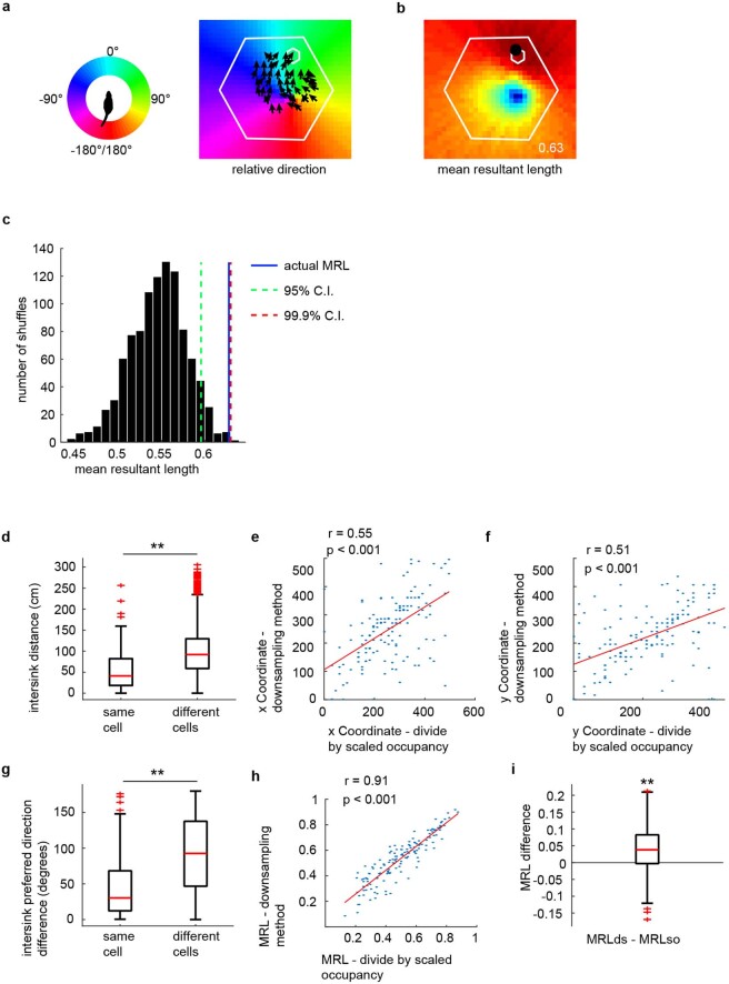
Extended Data Fig. 5. Calculation of the ConSink.
a, Left, each division of the colour wheel represents 1 search position in a polar co-ordinate framework centred on the animal’s head with 0° straight ahead. Right, the spatial environment is tiled by candidate sink positions. At each candidate position, the direction of all spikes relative to that position can be calculated (by subtracting the direction of the vector from the animal to the candidate position from the animal’s allocentric head direction). From this, a mean direction can be calculated, and is plotted here according to the colour wheel at left. The vector field (i.e. the mean allocentric direction of spikes at binned spatial positions) of an example ConSink cell (Rat 2, cell TT18c1) is overlaid. b, At each candidate sink position, the mean resultant length (MRL) of the associated distribution of relative directions is calculated (candidate positions are colour coded by MRL value). The candidate position with the largest MRL, which indicates the concentration of the polar distribution in the mean direction for that position, is taken as the ConSink (black closed circle; MRL = 0.63). c, To determine whether a cell was significantly modulated by relative direction to the candidate position identified as in (b), we shuffled the allocentric head directions associated with each spike, and recalculated relative direction MRLs at each search position, using the maximal MRL for our control distribution. This procedure was repeated 1000 times, and confidence intervals constructed. A cell was deemed to be significantly modulated if it’s MRL was greater than the 95th percentile of the shuffled distribution of maximal MRLs. d, To confirm the validity of our calculations, we recalculated the sinks in our identified ConSink cells using a downsampling method, in which, for each cell on each platform, the spikes were downsampled according to the directional occupancy in allocentric coordinates (see Methods). We then compared the distances between the sinks calculated with the 2 different methods (our “divide by scaled occupancy” method, and “downsampling” method) within and between cells. We found that sink positions were more similar within cells than across cells (Wilcoxson rank sum test, two-sided, n = 142 cells (same cells) or 20,022 pairs of cells (different cells) from 5 animals, z = −10.04, p = 9.94 x 10⁻²⁴), and x (e, Pearson correlation, r = 0.55, p = 1.50 x 10⁻¹²) and y coordinates (f, Pearson correlation, r = 0.51, p = 1.02 x 10⁻¹²) were strongly correlated across the two techniques. g, Similarly, preferred relative direction was more similar within cells (Wilcoxson rank sum test, two-sided, n = 142 cells (same cells) or 20,022 pairs of cells (different cells) from 5 animals, z = −9. 65, p = 5.07 x 10⁻²²). h, The strength of tuning was also highly correlated between the two techniques (Pearson correlation, r = 0.91, p = 7.99 x 10−55). i, Lastly, we found that our technique did not overestimate the strength of tuning, as tuning was slightly, but significantly, stronger in the downsampled data (Wilcoxson signed rank test, two-sided, n = 142 cells from 5 animals, z = 5.60, p = 2.18 x 10⁻⁸). For box plots in (d), (g) and (i), the central mark indicates the median, and the bottom and top edges of the box indicate the 25th and 75th percentiles, respectively; the whiskers extend to the most extreme data points within 1.5 times the interquartile range away from the bottom or top of the box, and all more extreme points are plotted individually using the ‘+’ symbol.

