An Elementary Solution to a Duffing Equation

Abstract

In this work, we study the Duffing equation. Analytical solution for undamped and unforced case is provided for any given arbitrary initial conditions. An approximate analytical solution is given for the damped or trigonometrically forced Duffing equation for arbitrary initial conditions. The analytical solutions are expressed in terms of elementary trigonometric functions as well as in terms of the Jacobian elliptic functions. Examples are added to illustrate the obtained results. We also introduce new functions for approximating the Jacobian and Weierstrass elliptic functions in terms of the trigonometric functions sine and cosine. Results are high accurate.

1. Introduction

Many physical phenomena are modeled by nonlinear systems of ordinary differential equations. The Duffing equation is an externally forced and damped oscillator equation that exhibits a range of interesting dynamic behavior in its solutions. The Duffing oscillator is an important model of nonlinear and chaotic dynamics. It was introduced by Germanic engineer Duffing in 1918 [1]. The Duffing oscillator is described by the differential equation:

$$\begin{array}{c}\ddot{x}+r\dot{x}+{\omega }_0^{2}x+\beta x^3=F\cos \omega t.\end{array}$$ (1)

It differs from the classical forced and damped harmonic oscillator only by the nonlinear term βx³, which changes the dynamics of the system drastically. Motivated by potential applications in physics, engineering, biology, and communication theory, the damped Duffing equation

$$\begin{array}{c}\ddot{x}+r\dot{x}+{\omega }_0^{2}x+\beta x^3=0,\end{array}$$ (2)

is considered. Equation (2) is a ubiquitous model arising in many branches of physics and engineering, such as the study of oscillations of a rigid pendulum undergoing with moderately large amplitude motion [2, 3], vibrations of a buckled beam, and so on [3–5].

It has provided a useful paradigm for studying nonlinear oscillations and chaotic dynamical systems, dating back to the development of approximate analytical methods based on perturbative ideas [2], and continuing with the advent of fast numerical integration by the computer, to be used as an archetypal illustration of chaos [2, 5–7]. Various methods for studying the damped Duffing equation and the forced Duffing equation (1) in feedback control, strange attractor, stability, periodic solutions, and numerical simulations have been proposed, and a vast number of profound results have been established [2].

The Duffing equation has been studied extensively in the literature. However, only few works are devoted to the study of its analytical solutions not using perturbation methods [8, 9]. Our aim is to avoid using such perturbation methods. This study is organized as follows. In the first section, we give exact analytical solution for the undamped and unforced Duffing equation for any given arbitrary initial conditions. In the second section, we provide formulas for obtaining a good approximate analytical solution using a new ansatz. The problems are solved for any arbitrary initial conditions. Finally, in the last section, we give approximate analytical solution to (1) and we compare it with Runge–Kutta numerical solution. Other useful methods are the homotopy perturbation method (HPM) [10–17], the Lindstedt–Poincaré method, and the Krylov–Bogoliubov–Mitropolsky method. The importance of numerical solution of differential equations in different fields of science and engineering is given in [18, 19].

2. Undamped and Unforced Duffing Equation

This is the equation:

$$\begin{array}{c}\ddot{x}+px+q{x}^3=0,x=x\left(t\right),\end{array}$$ (3)

and given the initial conditions,

$$\begin{array}{c}x\left(0\right)=x_0\text{\hspace{0.17em}and\hspace{0.17em}}{x}^{\prime }\left(0\right)={\dot{x}}_0\text{.}\end{array}$$ (4)

The general solution to equation (3) may be written in terms of any of the twelve Jacobian elliptic functions [20]. Let, for example,

$$\begin{array}{c}x\left(t\right)=c_1\text{cn}\left(\sqrt{\omega }t+c_2,m\right).\end{array}$$ (5)

Then,

$$\begin{array}{c}\ddot{x}+px+q{x}^3=\left(c_1^{3}q-2c_{1}m\omega \right)c{n}^3+\left(2c_{1}m\omega +c_{1}p-c_1\omega \right)cn,\text{where\hspace{0.17em}}cn=cn\left(\sqrt{\omega }t+c_2,m\right).\end{array}$$ (6)

Equating to zero, the coefficients of cn^j to zero gives an algebraic system whose solution is

$$\begin{array}{c}\omega =\sqrt{p+q{c}_1^2}\text{\hspace{0.17em}and\hspace{0.17em}}m=\frac{q{c}_1^2}{2\left(p+q{c}_1^2\right)}\text{.}\end{array}$$ (7)

Thus, the general solution to the Duffing equation is

$$\begin{array}{c}x\left(t\right)=cn\left(\sqrt{p+q{c}_1^2}t+c_2,\frac{q{c}_1^2}{2\left(p+q{c}_1^2\right)}\right).\end{array}$$ (8)

The values for the constants c₁ and c₂ are determined from the initial conditions.

Definition 1 . —

The number $\mathrm{\Delta }={\left(p+q{x}_0^2\right)}^2+2q{\dot{x}}_0^2$ is called the discriminant for the Duffing equations (3) and (4).

We will distinguish three cases depending on the sign of the discriminant [20].

2.1. First Case: Δ > 0

The solution to the i.v.p. (3) and (4) is given by

$$\begin{array}{c}x\left(t\right)=\sqrt{\frac{\sqrt{\mathrm{\Delta }}-p}{q}}cn\left(\sqrt[4]{\mathrm{\Delta }t}-\text{sign}\left({\dot{x}}_0\right)c{n}^{-1}\left(\sqrt{\frac{q}{\sqrt{\mathrm{\Delta }}-p}}{x}_0,\frac{1}{2}-\frac{p}{2\sqrt{\mathrm{\Delta }}}\right),\frac{1}{2}-\frac{p}{2\sqrt{\mathrm{\Delta }}}\right).\end{array}$$ (9)

Making use of the addition formula,

$$\begin{array}{c}cn\left(x+y,m\right)=\frac{cn\left(x,m\right)cn\left(y,m\right)+sn\left(x,m\right)dn\left(x,m\right)sn\left(y,m\right)dn\left(y,m\right)}{1-msn\left(x,m\right)sn\left(y,m\right)}.\end{array}$$ (10)

The solution (9) may be expressed as

$$\begin{array}{c}x\left(t\right)=\frac{x_0\text{cn}\left(\sqrt[4]{\mathrm{\Delta }t}|m\right)+\left({\dot{x}}_0/\sqrt[4]{\mathrm{\Delta }}\right)\text{sn}\left(\sqrt[4]{\mathrm{\Delta }t}|m\right)\text{dn}\left(\sqrt[4]{\mathrm{\Delta }t}|m\right)}{1+\left(\left(p+q{x}_0^2/2\sqrt{\mathrm{\Delta }}\right)-\left(1/2\right)\right)\text{sn}{\left(\sqrt[4]{\mathrm{\Delta }t}|m\right)}^2},\end{array}$$ (11)

where

$$\begin{array}{c}m=\frac{1}{2}\left(1-\frac{p}{\sqrt{\mathrm{\Delta }}}\right).\end{array}$$ (12)

Solution (11) is a periodic solution with period

$$\begin{array}{c}T=4\left|\frac{K\left(\left(1/2\right)\left(1-\left(p/\sqrt{\mathrm{\Delta }}\right)\right)\right)}{\sqrt[4]{\mathrm{\Delta }}}\right|.\end{array}$$ (13)

Example 1 . —

Let us consider the i.v.p.

$$\begin{array}{c}\left\{\begin{array}{c}{x}^{″}\left(t\right)+x\left(t\right)+x^3\left(t\right)=0,\hfill \\ x\left(0\right)=1\&x^{\prime }\left(0\right)=-1.\hfill \end{array}\right.\end{array}$$ (14)

Using formula (9), the exact solution to (14) is given by

$$\begin{array}{c}x\left(t\right)=\sqrt{\sqrt{6}-1}cn\left(\sqrt[4]{6t}-c{n}^{-1}\left(\frac{1}{\sqrt{-1+\sqrt{6}}},\frac{1}{2}-\frac{1}{2\sqrt{6}}\right)|\frac{1}{2}-\frac{1}{2\sqrt{6}}\right).\end{array}$$ (15)

According to the relations (11) and (12), the exact solution to the i.v.p. (14) may also be written as

$$\begin{array}{c}x\left(t\right)=\frac{cn\left(\sqrt[4]{6t}|\left(1/2\right)|\left(1-\left(1/\sqrt{6}\right)\right)\right)+\sqrt[4]{6dn}\left(\sqrt[4]{6t}|\left(1/2\right)|\left(1-\left(1/\sqrt{6}\right)\right)\right)sn\left(\sqrt[4]{6t}|\left(1/2\right)|\left(1-\left(1/\sqrt{6}\right)\right)\right)}{1+\left(\left(2-\sqrt{6}\right)/2\sqrt{6}\right)sn{\left(\sqrt[4]{6t}|\left(1/2\right)|\left(1-\left(1/\sqrt{6}\right)\right)\right)}^2}.\end{array}$$ (16)

The period is given by

$$\begin{array}{c}T=\frac{2\sqrt[4]{8}}{\sqrt[4]{3}}K\left(\frac{1}{2}\left(1-\frac{1}{\sqrt{6}}\right)\right)\approx \mathrm{4.37417.}\end{array}$$ (17)

In Figure 1, the comparison between the exact analytical solution (??) and the approximate numerical RK4 solution is presented. Full compatibility between the two analytical and numerical solutions is observed.

Figure 1.

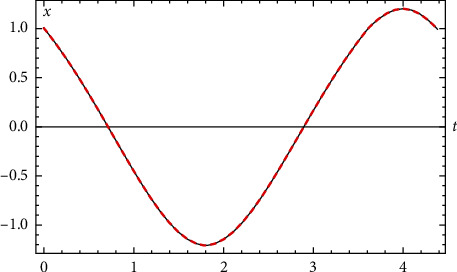
Comparison between the exact solution and the numerical solution for Example 1.

2.2. Second Case: Δ < 0

In this case, q < 0. Define

$$\begin{array}{c}\delta =-\frac{2p{x}_0^2+q{x}_0^4+2{\dot{x}}_0^2}{q}.\end{array}$$ (18)

Observe that

$$\begin{array}{c}\delta =\frac{p^2-\mathrm{\Delta }}{q^2}>0.\end{array}$$ (19)

Let

$$\begin{array}{c}x\left(t\right)=c-\frac{2c}{1+y\left(t\right)},\end{array}$$ (20)

where y=y(t) is a solution to Duffing equation

$$\begin{array}{c}{y}^{\prime \prime }\left(t\right)+ay\left(t\right)+b{y}^3\left(t\right)\end{array}$$ (21)

with initial conditions

$$\begin{array}{c}y\left(0\right)=y_0=\frac{2c{\dot{x}}_0}{{\left(c-x_0\right)}^2}\text{\hspace{0.17em}and\hspace{0.17em}}y\prime \left(0\right)={\dot{y}}_0=\frac{c+x_0}{c-x_0}.\end{array}$$ (22)

Inserting ansatz (21) into the ode x′′(t)+px(t)+qx³(t)=0 and taking into account the relation,

$$\begin{array}{c}{y}^{\prime }{\left(t\right)}^2={\dot{y}}_0+a{y}_0^2+\frac{b}{2}{y}_0^4-a{y}^2\left(t\right)-\frac{b}{2}{y}^4\left(t\right),\end{array}$$ (23)

we get

$$\begin{array}{c}\frac{cy\left(t\right)-c-x_{0}y\left(t\right)-x_0}{4{\left(c-x_0\right)}^4{\left(y\left(t\right)+1\right)}^4}\left(\ddot{x}+px+q{x}^3\right)=\left(\begin{array}{c}8a{c}^5-8a{c}^4{x}_0-8a{c}^3{x}_0^2+8a{c}^2{x}_0^3+4b{c}^5+12b{c}^4{x}_0+12b{c}^3{x}_0^2+4b{c}^2{x}_0^3+c^{7}q-5c^{6}q{x}_0+2c^{5}p\\ +11c^{5}q{x}_0^2-10c^{4}p{x}_0-15c^{4}q{x}_0^3+20c^{3}p{x}_0^2+15c^{3}q{x}_0^4+30c^3{\dot{x}}_0^2-20c^{2}p{x}_0^3-11c^{2}q{x}_0^5\\ -22c^2{x}_0{\dot{x}}_0^2+10cp{x}_0^4+5cq{x}_0^6+10c{x}_0^2{\dot{x}}_0^2-2p{x}_0^5-q{x}_0^7-2x_0^3{\dot{x}}_0^2\end{array}\right)\\ +\left(c-x_0\right)\left(\begin{array}{c}8a{c}^4-16a{c}^3{x}_0+8a{c}^2{x}_0^2+4b{c}^4+8b{c}^3{x}_0+4b{c}^2{x}_0^2-3c^{6}q+10c^{5}q{x}_0+2c^{4}p-11c^{4}q{x}_0^2-\\ 12c^{3}p{x}_0+24c^{2}p{x}_0^2+11c^{2}q{x}_0^4+22c^2{\dot{x}}_0^2-20cp{x}_0^3-10cq{x}_0^5-20c{x}_0{\dot{x}}_0^2+6p{x}_0^4+3q{x}_0^6+6x_0^2{\dot{x}}_0^2\end{array}\right)y\left(t\right)\\ +{\left(c-x_0\right)}^2\left(4b{c}^3+4b{c}^2{x}_0+3c^{5}q-5c^{4}q{x}_0-2c^{3}p-2c^{2}p{x}_0+10cp{x}_0^2+5cq{x}_0^4+10c{\dot{x}}_0^2-6p{x}_0^3-3q{x}_0^5-6x_0{\dot{x}}_0^2\right)y^2\left(t\right)+{\left(c-x_0\right)}^3\left(4b{c}^2-q{c}^4-2c^{2}p+2p{x}_0^2+q{x}_0^4+2{\dot{x}}_0^2\right)y^3\left(t\right).\end{array}$$ (24)

Equating to zero, the coefficients of y^j(t) give an algebraic system. A solution to this system is

$$\begin{array}{c}a=\frac{1}{2}\left(-p-3\sqrt{\delta }q\right),b=\frac{1}{2}\left(p-\sqrt{\delta }q\right),c=\sqrt[4]{\delta }.\end{array}$$ (25)

Observe that the Duffing equations (21) and (22) have a positive discriminant given by

$$\begin{array}{c}{\left(a+b{y}_0^2\right)}^2+2b{\dot{y}}_0^2=\frac{\delta {\left(c-x_0\right)}^4\left(2c^4{\dot{x}}_0^2+\delta {\left(c^2+x_0^2\right)}^2\right)}{4c^8{x}_0^2}.\end{array}$$ (26)

Then, the problem reduces to the first case.

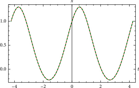
Example 2 . —

Let us assume the following i.v.p.:

$$\begin{array}{c}{x}^{\prime \prime }\left(t\right)+2x\left(t\right)-x^3\left(t\right)=0,x\left(0\right)=-1\text{\hspace{0.17em}and\hspace{0.17em}}{x}^{\prime }\left(0\right)=1.\end{array}$$ (27)

The solution of i.v.p. (27) according to the relation (??) reads

$$\begin{array}{c}x\left(t\right)=1.49535-\frac{2.9907}{1+\left(\left(0.198509cn\left(2.08627t|1.00018\right)-0.230219dn\left(2.08627t|1.00018\right)sn\left(2.08627t|1.00018\right)\right)/1-1.00072sn{\left(2.08627t|1.00018\right)}^2\right)}.\end{array}$$ (28)

The period of solution (28) is given by

$$\begin{array}{c}T=\frac{4K\left(1/m\right)}{w\sqrt{m}}=10.9034\left(\text{for\hspace{0.17em}}m=1.00018\text{\hspace{0.17em}and\hspace{0.17em}}w=2.08627\right).\end{array}$$ (29)

Comparison between the exact solution and numerical solution is shown in Figure 2.

Figure 2.

Comparison between the exact solution and the numerical solution for Example 2.

2.3. Third Case: Δ=0 and p ≠ 0

If the discriminant vanishes (Δ=0), then q < 0, and the only solution to problem (??) with

$$\begin{array}{c}{x}^{\prime }{\left(0\right)}^2={\dot{x}}_0^2=\frac{{\left(p+q{y}_0^2\right)}^2}{-2q}\end{array}$$ (30)

reads

$$\begin{array}{c}x\left(t\right)=\sqrt{-\frac{p}{q}}\tanh \left[\sqrt{\frac{p}{2}}t\pm {\tanh }^{-1}\left(x_0\sqrt{-\frac{q}{p}}\right)\right],\end{array}$$ (31)

which may be verified by direct computation.

2.4. Fourth Case: Δ=0 and p=0

The solution is given by

$$\begin{array}{c}x\left(t\right)=\frac{2x_0}{2+\sqrt{-2q}{x}_{0}t}.\end{array}$$ (32)

Remark 1 . —

The solution to the i.v.p.

$$\begin{array}{c}\ddot{x}+px+q{x}^3=0\text{,\hspace{0.17em}}x\left(0\right)=x_0\text{\hspace{0.17em}and\hspace{0.17em}}{x}^{\prime }\left(0\right)=0,\end{array}$$ (33)

is

$$\begin{array}{c}x\left(t\right)=x_{0}cn\left(\sqrt{p+q{x}_0^2},\frac{q{x}_0^2}{2\left(p+q{x}_0^2\right)}\right).\end{array}$$ (34)

Remark 2 . —

Let $p+\sqrt{p^2+2q{\dot{x}}_0^2}>0$. Then, the solution to the i.v.p.

$$\begin{array}{c}\ddot{x}+px+q{x}^3=0,x\left(0\right)=0\text{\hspace{0.17em}and\hspace{0.17em}}x\prime \left(0\right)={\dot{x}}_0,\end{array}$$ (35)

is

$$\begin{array}{c}x\left(t\right)=\frac{\sqrt{2}{\dot{x}}_0}{\sqrt{\sqrt{p^2+2q{\dot{x}}_0^2}+p}}sn\left(\sqrt{\frac{p+\sqrt{p^2+2q{\dot{x}}_0^2}}{2}}t,-\frac{p^2+q{\dot{x}}_0^2-\sqrt{p^2+2q{\dot{x}}_0^2}p}{q{\dot{x}}_0^2}\right).\end{array}$$ (36)

Remark 3 . —

Using the identity

$$\begin{array}{c}cn\left(\sqrt{\omega }t,m\right)=1-\frac{6}{\left(4m+1\right)\left(1+12/\left(4m+1\right)\omega \wp \left(t;1/12\left(16m^2-16m+1\right){\omega }^2,1/216\left(2m-1\right)\left(32m^2-32m-1\right){\omega }^3\right)\right)},\end{array}$$ (37)

the solution to the Duffing equations (3) and (4) may be written in terms of the Weierstrass elliptic function ℘. More precisely, if Δ > 0, then

$$\begin{array}{c}x\left(t\right)=A-\frac{A\left(2+\left(4p/3A^{2}q+p\right)\right)}{1+\left(12/3A^{2}q+p\right)\wp \left(t+t_0;\left(1/12\right)\left(-3q^2{A}^4-6pq{A}^2+p^2\right),\left(1/216\right)p\left(9q^2{A}^4+18pq{A}^2+p^2\right)\right)},\end{array}$$ (38)

where

$$\begin{array}{c}{t}_0={\wp }^{-1}\left(\frac{3A^{3}q+3A^{2}q{x}_0+5Ap+p{x}_0}{12\left(A-x_0\right)};\frac{1}{12}\left(-3A^4{q}^2-6A^{2}pq+p^2\right),\frac{1}{216}p\left(9A^4{q}^2+18A^{2}pq+p^2\right)\right),\end{array}$$ (39)

$$\begin{array}{c}A=\sqrt{\frac{-p\pm \sqrt{{\left(p+q{x}_0^2\right)}^2+2q{\dot{x}}_0^2}}{q}}=\pm \sqrt{\frac{-p\pm \sqrt{\mathrm{\Delta }}}{q}}.\end{array}$$ (40)

The solution (38) is periodic with period

$$\begin{array}{c}T=2{\displaystyle {\int }_{\rho }^{+\infty }\frac{dx}{\sqrt{4x^3-g_{2}x-g_3}}},\end{array}$$ (41)

where ρ is the greatest real root to the cubic 4x³ − g₂x − g₃=0 and

$$\begin{array}{c}{g}_2=\frac{1}{12}\left(-3q^2{A}^4-6pq{A}^2+p^2\right)\text{\hspace{0.17em}and\hspace{0.17em}}{g}_3=\frac{1}{216}p\left(9A^4{q}^2+18A^{2}pq+p^2\right).\end{array}$$ (42)

On the other hand,

$$\begin{array}{c}\wp \left(t;g_2,g_3\right)=\frac{\sqrt{3g_2}}{\sqrt{16m^2-16m+1}\left(1-cn\left(\sqrt{2}\sqrt[4]{3g_2/16m^2-16m+1}t,m\right)\right)}-\frac{\sqrt{g_2}\left(4m+1\right)}{2\sqrt{48m^2-48m+3}},\end{array}$$ (43)

where m is a root to the sextic

$$\begin{array}{c}4096\left(g_2^3-27g_3^2\right)z^6-12288\left(g_2^3-27g_3^2\right)z^5+13056\left(g_2^3-27g_3^2\right)z^4-5632\left(g_2^3-27g_3^2\right)z^3+12\left(59g_2^3-1836g_3^2\right)z^2+12\left(5g_2^3+108g_3^2\right)z+g_2^3-27g_3^2=0.\end{array}$$ (44)

Thus,

$$\begin{array}{c}{\displaystyle {\int }_{\rho }^{+\infty }\frac{dx}{\sqrt{4x^3-g_{2}x-g_3}}}=\sqrt{2}\sqrt[4]{\frac{16m^2-16m+1}{3g_2}}K\left(m\right)\text{\hspace{0.17em}for\hspace{0.17em}}m<1.\end{array}$$ (45)

3. Approximate Analytical Solution Using Elementary Functions

We define the generalized sine and cosine functions as follows:

$$\begin{array}{c}{\sin }_m\left(t\right)=\frac{\sin \left(\sqrt{1+\kappa }t\right)}{\sqrt{1+\kappa {\cos }^2\left(\sqrt{1+\kappa }t\right)}},\end{array}$$ (46)

$$\begin{array}{c}{\cos }_m\left(t\right)=\frac{\sqrt{1+\kappa }\cos \left(\sqrt{1+\kappa }t\right)}{\sqrt{1+\kappa {\cos }^2\left(\sqrt{1+\kappa }t\right)}},\end{array}$$ (47)

$$\begin{array}{c}\kappa =\frac{1}{14}\left(m-12+\sqrt{144-144m+m^2}\right).\end{array}$$ (48)

These functions are good approximations to the Jacobian elliptic functions sn and cn for −1 ≤ m ≤ 1/2. For example, let

$$\begin{array}{c}T=2K\left(m\right)\approx \frac{\pi }{\sqrt{1+\kappa }}.\end{array}$$ (49)

Then,

$$\begin{array}{c}{\text{Max}}_{-T\le t\le T,-1\le m\le \left(1/2\right)}\left|\text{sn}\left(t,m\right)-{\sin }_{\text{m}}\left(\text{t}\right)\right|=0.00290582,\end{array}$$ (50)

$$\begin{array}{c}{\text{Max}}_{-T\le t\le T,-1\le m\le 1/2}\left|cn\left(t,m\right)-{\cos }_m\left(t\right)\right|=\mathrm{0.00541969.}\end{array}$$ (51)

Table 1 provides the errors for different values of m.

Table 1.

Errors for approximations (46) and (47).

m	Max−T≤t≤T|sn(t, m) − sinm(t)|	Max−T≤t≤T|cn(t, m) − cosm(t)|
0	0	0
0.05	0.0000186142	0.0000332484
0.1	0.0000775641	0.000139051
0.15	0.000182102	0.000327722
0.2	0.000338416	0.000611534
0.25	0.000553861	0.00100522
0.3	0.000837256	0.00152665
0.35	0.0011993	0.00219775
0.4	0.00165312	0.00304575
0.45	0.00221506	0.00410502
0.5	0.00290582	0.00541969
0.55	0.00375209	0.00704758
0.6	0.00478916	0.0.0090664
0.66	0.00606499	0.0115838
0.7	0.00764718	0.0147546
0.75	0.00963546	0.0188129
0.8	0.0121865	0.0241364
0.85	0.055962	0.0313949
0.9	0.0203137	0.0419635
0.95	0.0277681	0.0595356

More accurate approximations are obtained by letting

$$\begin{array}{c}{\sin }_m\left(t\right)=\frac{\sin \left(\sqrt{1+\kappa }t\right)}{\sqrt{1+\kappa {\cos }^2\left(\sqrt{1+\kappa }t\right)+\mu {\cos }^4\left(\sqrt{1+\kappa }t\right)}},\end{array}$$ (52)

$$\begin{array}{c}{\cos }_m\left(t\right)=\frac{\sqrt{1+\kappa +\mu }\cos \left(\sqrt{1+\kappa }t\right)}{\sqrt{1+\kappa {\cos }^2\left(\sqrt{1+\kappa }t\right)+\mu {\cos }^4\left(\sqrt{1+\kappa }t\right)}},\end{array}$$ (53)

$$\begin{array}{c}{\sin }_m\left(t\right)=\frac{\sin \left(t\sqrt{-\kappa -\mu -1}/\sqrt{\mu -1}\right)\sqrt{1-\mu {\cos }^2\left(t\sqrt{-\kappa -\mu -1}/\sqrt{\mu -1}\right)}}{\sqrt{\mu {\cos }^4\left(t\sqrt{-\kappa -\mu -1}/\sqrt{\mu -1}\right)+\kappa {\cos }^2\left(t\sqrt{-\kappa -\mu -1}/\sqrt{\mu -1}\right)+1}}.\end{array}$$ (54)

$$\begin{array}{c}\kappa =\frac{\left(\sqrt{\begin{array}{c}\left(5184m^2-14256m+15633\right){\mu }^4+\left(-24192m^2+92016m-89856\right){\mu }^3+\\ \left(42048m^2-211392m+193536\right){\mu }^2+\left(-32256m^2+207360m-184320\right)\mu \\ +9216m^2-73728m+65536\end{array}}\right)+\left(-72m-9\right){\mu }^2+\left(168m-960\right)\mu -96m-256}{48\left(3\mu +10\right)}\end{array}$$ (55)

$$\begin{array}{c}\mu =\frac{4m^2\left(1061m^4-7768m^3+24128m^2-32768m+16384\right)}{10521m^6-136752m^5+786336m^4-2345984m^3+3792896m^2-3145728m+1048576}.\end{array}$$ (56)

For these new approximations, we will have

$$\begin{array}{c}{\text{Max}}_{-T\le t\le T,-1\le m\le 0.9}\left|sn\left(t,m\right)-{\sin }_m\left(t\right)\right|=0.0607706,\end{array}$$ (57)

$$\begin{array}{c}{\text{Max}}_{-T\le t\le T,-1\le m\le 0.9}\left|cn\left(t,m\right)-{\cos }_m\left(t\right)\right|=\mathrm{0.030797.}\end{array}$$ (58)

Table 2 provides the errors for different values of m.

Table 2.

Errors for approximations (52) and (53).

m	Max−T≤t≤T|sn(t, m) − sinm(t)|	Max−T≤t≤T|cn(t, m) − cosm(t)|
0	0	0
0.05	8.066e-9	6.548e-9
0.1	1.4551e-7	1.158e-7
0.15	8035e-7	6.51e-7
0.2	3.0125e-6	2.23e-6
0.25	8.45e-6	6.29e-6
0.3	0.00002	0.000015
0.35	0.00004	0.000031
0.4	0.000089	0.000061
0.45	0.00017	0.00011
0.5	0.00032	0.00021
0.55	0.00058	0.00037
0.6	0.0011	0.00065
0.65	0.0019	0.0012
0.7	0.0036	0.0021
0.75	0.0071	0.0039
0.8	0.0146	0.0079
0.85	0.0327	0.0173
0.9	0.0832	0.043
0.95	0.265	0.136

From Tables 1 and 2, it is seen that for the values 0.8 < m < 1, the approximations (46) and (47) are better than (53) and (54). Thus, we have

$$\begin{array}{c}sn\left(t,m\right)\approx {\sin }_m\left(t\right),cn\left(t,m\right)\approx {\cos }_m\left(t\right)\text{\hspace{0.17em}and\hspace{0.17em}}dn\left(t,m\right)\approx \sqrt{1-ms{n}^2\left(t,m\right)}=d{n}_m\left(t\right)\text{\hspace{0.17em}for\hspace{0.17em}}-1\le m<1.\end{array}$$ (59)

We may write approximate elementary solution to Duffing equations (3) and (4) as follows:

$$\begin{array}{c}x\left(t\right)=\frac{x_0{\cos }_m\left(\sqrt[4]{\mathrm{\Delta }t}\right)+{\dot{x}}_0/\sqrt[4]{\mathrm{\Delta }}{\sin }_m\left(\sqrt[4]{\mathrm{\Delta }t}\right){\text{dn}}_m\left(\sqrt[4]{\mathrm{\Delta }t}\right)}{1+\left(\left(p+q{x}_0^2/2\sqrt{\mathrm{\Delta }}\right)-\left(1/2\right)\right){\sin }_m{\left(\sqrt[4]{\mathrm{\Delta }t}\right)}^2},\end{array}$$ (60)

where

$$\begin{array}{c}m=\frac{1}{2}\left(1-\frac{p}{\sqrt{\mathrm{\Delta }}}\right),p>0,\mathrm{\Delta }={\left(p+q{x}_0^2\right)}^2+2q{\dot{x}}_0^2>0.\end{array}$$ (61)

$$\begin{array}{c}x\left(t\right)=A-\frac{2A}{1+B\left(b_0{\cos }_m\left(\sqrt{\omega }t\right)+b_1{\sin }_m\left(\sqrt{\omega }t\right)d{n}_m\left(\sqrt{\omega }t\right)/1+b_2{\sin }_m{\left(\sqrt{\omega }t\right)}^2\right)},\mathrm{\Delta }<0.\end{array}$$ (62)

The values for the constants in (62) are the same as in (??).

Remark 4 . —

In the case when |m| > 1, we use the approximations:

$$\begin{array}{c}cn\left(t,m\right)\approx d{n}_{1/m}\left(\sqrt{m}t\right),\end{array}$$ (63)

$$\begin{array}{c}sn\left(t,m\right)\approx \sqrt{\frac{1}{m}}{\sin }_{1/m}\left(\sqrt{m}t\right),\end{array}$$ (64)

$$\begin{array}{c}dn\left(t,m\right)\approx {\cos }_{1/m}\left(\sqrt{m}t\right).\end{array}$$ (65)

Then, formula (60) takes the following form when p < 0 and m > 1:

$$\begin{array}{c}x\left(t\right)=\frac{x_0{\text{dn}}_{1/m}\left(\sqrt[4]{\mathrm{\Delta }}\sqrt{m}t\right)+{\dot{x}}_0/\sqrt[4]{\mathrm{\Delta }}\sqrt{1/m}{\sin }_{\left(1/m\right)}\left(\sqrt{m}\sqrt[4]{\mathrm{\Delta }t}\right){\text{cos}}_{\left(1/m\right)}\left(\sqrt[4]{\mathrm{\Delta }}\sqrt{m}t\right)}{1+\left(1/m\right)\left(\left(p+q{x}_0^2/2\sqrt{\mathrm{\Delta }}\right)-\left(1/2\right)\right){\sin }_{1/m}^2\left(\sqrt[4]{\mathrm{\Delta }}\sqrt{m}t\right)}\text{,\hspace{0.17em}}\mathrm{\Delta }>0.\end{array}$$ (66)

Similar formula for (62) when Δ < 0.

In the case when 0.9 < m ≤ 1.1, we may use the following approximations:

$$\begin{array}{c}\left\{\begin{array}{c}cn\left(t,m\right)\approx \frac{1}{8}\left(m-1\right)\left(\sinh \left(2t\right)-2t\right)\tanh \left(t\right)\sec h\left(t\right)+\sec h\left(t\right),\hfill \\ sn\approx \frac{1}{4}\left(\left(m-1\right)t\sec h^2\left(t\right)-\left(m-5\right)\tanh \left(t\right)\right),\hfill \\ dn\approx \sec h\left(t\right)-\frac{1}{4}\left(m-1\right)\tanh \left(t\right)\left(\sinh \left(t\right)+t\sec h\left(t\right)\right).\hfill \end{array}\right.\end{array}$$ (67)

Example 3 . —

Let us return to Example 1.

$$\begin{array}{c}\left\{\begin{array}{c}{x}^{\prime \prime }\left(t\right)+x\left(t\right)+x^3\left(t\right)=0,\hfill \\ x\left(0\right)=1\&x^{\prime }\left(0\right)=-1.\hfill \end{array}\right.\end{array}$$ (68)

The approximate elementary analytical solution is

$$\begin{array}{c}{x}_{app}\left(t\right)=\frac{\left(\left(3.4319\cos \left(1.43552t\right)\right)/\sqrt{14.-2.22208{\cos }^2\left(1.43552t\right)}\right)-\left(0.638943\sin \left(1.43552t\right)\sqrt{1+\left(4.14226{\sin }^2\left(1.43552t\right)/2.22208{\cos }^2\left(1.43552t\right)-14.\right)}/\sqrt{1.-0.15872{\cos }^2\left(1.43552t\right)}\right)}{1-\left(0.0917517{\sin }^2\left(1.43552t\right)/1.-0.15872{\cos }^2\left(1.43552t\right)\right)}.\end{array}$$ (69)

The exact period is given by T=4.37417. The approximate period is that of (59), and it is given by

$$\begin{array}{c}{T}_{\text{app}}=\frac{2\pi }{1.4355163606}=\mathrm{4.37695.}\end{array}$$ (70)

This value differs from the exact value by 0.00278457. The error of the approximate solution comparted with exact solution is

$$\begin{array}{c}{\max }_{-T/2\le t\le T/2}\left|x_{\text{app}}\left(t\right)-x_{\text{exact}}\left(t\right)\right|=\mathrm{0.001847.}\end{array}$$ (71)

Comparison between the exact solution and the approximate analytical solution is shown in Figure 3.

Figure 3.

Comparison between the exact solution and the approximate analytical solution for Example 3.

Example 4 . —

Let us return to Example 2. Let (Figure 4)

$$\begin{array}{c}{x}^{\prime \prime }\left(t\right)+2x\left(t\right)-x^3\left(t\right)=0,x\left(0\right)=-1\text{\hspace{0.17em}and\hspace{0.17em}}x\left(0\right)=1.\end{array}$$ (72)

Figure 4.

Comparison between the exact solution and the approximate analytical solution for Example 4.

Remark 5 . —

From (47)–(44) or (53)–(44), we obtain the following approximate expression for the Weierstrass elliptic function by means of the cosine function:

$$\begin{array}{c}\wp \left(t;g_2,g_3\right)=\frac{\sqrt{3g_2}}{\sqrt{16m^2-16m+1}\left(1-{\text{\hspace{0.17em}\hspace{0.17em}cos}}_m\left(\sqrt{2}\sqrt[4]{3g_2/16m^2-16m+1}t\right)\right)}-\frac{\sqrt{g_2}\left(4m+1\right)}{2\sqrt{48m^2-48m+3}},\end{array}$$ (73)

where m is a root to the sextic (44).

Example 5 . —

Let g₂=2 and g₃=1. For this choice, m=0.0119056. We have

$$\begin{array}{c}\wp \left(t;\mathrm{2,1}\right)\approx \frac{2.71867}{1-\left(3.73048\cos \left(2.32484t\right)/\sqrt{14.-0.0835474{\cos }^2\left(2.32484t\right)}\right)}-\mathrm{0.474691.}\end{array}$$ (74)

The period is T=2.70262, and the error on the interval −(T/2) ≤ t ≤ (T/2) in the sup norm is E=8.52 × 10⁻⁷. Comparison between the approximate analytical solution and the numerical solution is shown in Figure 5. The reciprocals of the two functions are plotted on the interval −(T/2) ≤ t ≤ (T/2).

Figure 5.

Comparison between the approximate analytical solution and the numerical solution for Example 5.

4. Analytical Solution to a Generalized Duffing Equation

Let us consider the i.v.p. [21]:

$$\begin{array}{c}\ddot{u}+\alpha u+\beta u^3=F,\end{array}$$ (75)

given that

$$\begin{array}{c}u\left(0\right)=u_0\text{\hspace{0.17em}and\hspace{0.17em}}u\prime \left(0\right)={\dot{u}}_0.\end{array}$$ (76)

We will say that (75) is a constantly forced Duffing equation. When F=0, that becomes an undamped and unforced Duffing equation, and we already know how to solve it for arbitrary initial conditions. Let

$$\begin{array}{c}x\left(t\right)=\lambda +\frac{\mu }{1+\wp \left(\rho t+t_0;g_2,g_3\right)},\end{array}$$ (77)

where λ, μ, w, g₂, g₃, and t₀ are some constants to be determined. Plugging ansatz (77) into (75) gives

$$\begin{array}{c}\ddot{u}+\alpha u+\beta u^3-F=\frac{1}{2{\left(1+\wp \right)}^3}\left(\begin{array}{c}-2\left(F-\alpha \lambda -\beta {\lambda }^3-2\mu {\rho }^2\right)-2\left(3F-3\alpha \lambda -\alpha \mu -3\beta {\lambda }^3-3\beta {\lambda }^2\mu +6\mu {\rho }^2\right)\wp +\\ \left(-6F-3g_2\mu {\rho }^2+6\alpha \lambda +4\alpha \mu +6\beta {\lambda }^3+12\beta {\lambda }^2\mu +6\beta \lambda {\mu }^2\right){\wp }^2+\\ \left(-2F+g_2\mu {\rho }^2-4g_3\mu {\rho }^2+2\alpha \lambda +2\alpha \mu +2\beta {\lambda }^3+6\beta {\lambda }^2\mu +6\beta \lambda {\mu }^2+2\beta {\mu }^3\right){\wp }^3\end{array}\right),\end{array}$$ (78)

where ℘=℘(ρ t+t₀; g₂, g₃). Equating to zero, the coefficients of ℘^j (j=0,1,2,3) in the right-hand side of (78) gives an algebraic system. A nontrivial solution to this system is

$$\begin{array}{c}\left\{\begin{array}{c}\mu =\frac{6\left(F-\lambda \left(\alpha +\beta {\lambda }^2\right)\right)}{\alpha +3\beta {\lambda }^2},\rho =\frac{1}{2}\sqrt{\frac{\alpha }{3}+\beta {\lambda }^2},\hfill \\ g_2=12-\frac{144\beta \lambda \left(-F+\alpha \lambda +\beta {\lambda }^3\right)}{{\left(\alpha +3\beta {\lambda }^2\right)}^2},g_3=\frac{8\left(27F^2\beta +9\alpha \beta \lambda \left(\beta {\lambda }^3-4F\right)+{\alpha }^3+18{\alpha }^2\beta {\lambda }^2\right)}{{\left(\alpha +3\beta {\lambda }^2\right)}^3}.\hfill \end{array}\right.\end{array}$$ (79)

Now, to find the values of t₀ and λ, we make use of the addition formula:

$$\begin{array}{c}\wp \left(w+z;g_2,g_3\right)=\frac{1}{4}{\left(\frac{{\wp }^{\prime }\left(w;g_2,g_3\right)-{\wp }^{\prime }\left(z;g_2,g_3\right)}{\wp \left(w;g_2,g_3\right)-\wp \left(z;g_2,g_3\right)}\right)}^2-\wp \left(w;g_2,g_3\right)-\wp \left(z;g_2,g_3\right).\end{array}$$ (80)

We then find that

$$\begin{array}{c}{t}_0={\wp }^{-1}\left(\frac{u_0-\lambda -\mu }{\lambda -u_0};g_2,g_3\right).\end{array}$$ (81)

The number λ must be a solution to the quartic

$$\begin{array}{c}4F{u}_0-\beta u_0^4-2u_0^2\alpha -2{\dot{u}}_0^2-4F\lambda +2\alpha {\lambda }^2+\beta {\lambda }^4=0.\end{array}$$ (82)

Using (75), we also may obtain an approximate analytical solution in terms of the cosine function.

Remark 6 . —

The i.v.p.

$$\begin{array}{c}\ddot{x}+n+px+q{x}^2+r{x}^3=0\text{,\hspace{0.17em}}x=x\left(t\right),\end{array}$$ (83)

given the initial conditions

$$\begin{array}{c}x\left(0\right)=x_0\text{\hspace{0.17em}and\hspace{0.17em}}x\prime \left(0\right)={\dot{x}}_0,\end{array}$$ (84)

is a particular case of (75) and (76). Indeed, let x(t)=u(t) − (q/3r). Then, problems (83) and (84) reduce to the problem

$$\begin{array}{c}n+u\left(t\right)\left(p-\frac{q^2}{3r}\right)-\frac{pq}{3r}+\frac{2q^3}{27r^2}+ru{\left(t\right)}^3+u^{\prime \prime }\left(t\right)=0,\end{array}$$ (85)

$$\begin{array}{c}u\left(0\right)=x_0+\frac{q}{3r}\text{\hspace{0.17em}and\hspace{0.17em}}{u}^{\prime }\left(0\right)={\dot{x}}_0\text{.}\end{array}$$ (86)

Example 6 . —

Let

$$\begin{array}{c}\ddot{u}+u\left(t\right)+u^3\left(t\right)=1\wedge u\left(0\right)=1\wedge u^{\prime }\left(0\right)=1.\end{array}$$ (87)

The exact solution is

$$\begin{array}{c}{u}_{\text{exact}}\left(t\right)=0.29637-\frac{2.45792}{1+\wp \left(0.370192-0.709561t;-0.657491,1.34218\right)},\end{array}$$ (88)

with period

$$\begin{array}{c}{T}_{\text{exact}}=\mathrm{4.24726758.}\end{array}$$ (89)

An approximate analytical solution is

$$\begin{array}{c}{u}_{\text{app}}\left(t\right)=1.29637-\frac{2.45792}{0.474364+\left(2.28411/1-\left(3.64963\cos \left(0.771764-1.47927t\right)/\sqrt{14.-0.68022{\cos }^2\left(0.771764-1.47927t\right)}\right)\right)},\end{array}$$ (90)

with period

$$\begin{array}{c}{T}_{\text{app}}=\mathrm{4.24748881.}\end{array}$$ (91)

The error is

$$\begin{array}{c}{\max }_{-\left(T/2\right)\le t\le \left(T/2\right)}\left|u_{\text{exact}}\left(t\right)-u_{\text{app}}\left(t\right)\right|=\mathrm{0.000105178.}\end{array}$$ (92)

Comparison between the approximate analytical solution and the numerical solution is shown in Figure 6.

Figure 6.

Comparison between the approximate analytical solution and the numerical solution for Example 6.

5. Damped and Unforced Duffing Equation

Let us consider the i.v.p.

$$\begin{array}{c}\ddot{u}+2\epsilon \dot{u}+\alpha u+\beta u^3=0,\epsilon >\text{0,}\end{array}$$ (93)

given that

$$\begin{array}{c}u\left(0\right)=u_0\text{\hspace{0.17em}and\hspace{0.17em}}{u}^{\prime }\left(0\right)={\dot{u}}_0.\end{array}$$ (94)

We will suppose that lim_t⟶∞u(t)=0. Define the residual as

$$\begin{array}{c}R\left(t\right)=u^{\prime \prime }\left(t\right)+2\epsilon u^{\prime }\left(t\right)+pu\left(t\right)+q{u}^3\left(t\right).\end{array}$$ (95)

5.1. First Case: u₀ ≠ 0

Assume the ansatz

$$\begin{array}{c}u\left(t\right)=\exp \left(-\rho t\right)\frac{u_0\text{cn}\left(f\left(t\right),m\left(t\right)\right)+b_1\text{sn}\left(f\left(t\right),m\left(t\right)\right)\text{dn}\left(f\left(t\right),m\left(t\right)\right)}{1+b_2{\text{sn}}^2\left(f\left(t\right),m\left(t\right)\right)}.\end{array}$$ (96)

Then, from results in [22],

$$\begin{array}{c}{f}^{\prime }{\left(t\right)}^2=\alpha -2\epsilon \rho +{\rho }^2+\beta u_0^2{e}^{-2t\rho }\text{\hspace{0.17em}and\hspace{0.17em}}m\left(t\right)=\frac{\beta u_0^2{e}^{-2t\rho }}{2f^{\prime }{\left(t\right)}^2},\end{array}$$ (97)

so that

$$\begin{array}{c}f\left(t\right)=\frac{1}{\rho }\left(\sqrt{\beta u_0^2+\mu }-\sqrt{\beta u_0^2{e}^{-2t\rho }+\mu }+\sqrt{\mu }\left({\text{tanh}}^{-1}\left(\sqrt{1+\frac{\beta u_0^2{e}^{-2t\rho }}{\mu }}\right)-{\text{tanh}}^{-1}\left(\sqrt{1+\frac{\beta u_0^2}{\mu }}\right)\right)\right),\end{array}$$ (98)

$$\begin{array}{c}m\left(t\right)=\frac{1/2}{1+\left(\mu e^{2t\rho }/\beta u_0^2\right)},\end{array}$$ (99)

being

$$\begin{array}{c}\mu =\alpha -2\epsilon \rho +{\rho }^2.\end{array}$$ (100)

The numbers b₁, b₂, and ρ are obtained from the following conditions:

$$\begin{array}{c}\left\{\begin{array}{c}{u}^{\prime }\left(0\right)={\dot{u}}_0\text{,}\hfill \\ R\left(0\right)=0,\hfill \\ R^{\prime }\left(0\right)=0.\hfill \end{array}\right.\end{array}$$ (101)

Solving the two equations in (88) gives

$$\begin{array}{c}\left\{\begin{array}{c}{b}_1=\frac{u_0\rho +{\dot{u}}_0}{\sqrt{u_0^2\beta +\mu }}.\\ b_2=\frac{u_0^3\beta \left(3\alpha -4\epsilon \rho -3\mu \right)+{\dot{u}}_0\left(u_0^2\beta \left(2\epsilon -3\rho \right)+2\left(\epsilon -\rho \right)\left(\alpha +\rho \left(\rho -2\epsilon \right)\right)\right)+2u_0\rho \left(\epsilon -\rho \right)\left(\alpha +\rho \left(\rho -2\epsilon \right)\right)}{2u_0{\left(u_0^2\beta +\mu \right)}^2}\end{array}\right\}.\end{array}$$ (102)

The number ρ is a root to the septic

$$\begin{array}{c}-2\epsilon {\left(u_0^2\beta +\alpha \right)}^2\left(u_0^2\alpha +u_0^4\beta +2{\dot{u}}_0{u}_0\epsilon +3{\dot{u}}_0^2\right)\\ +\left(u_0^2\beta +\alpha \right)\left(\begin{array}{c}2u_0^2{\alpha }^2+5u_0^4\alpha \beta +8u_0^2\alpha {\epsilon }^2-4{\dot{u}}_0{u}_0\alpha \epsilon +6{\dot{u}}_0^2\alpha +\\ 3u_0^6{\beta }^2+8u_0^4\beta {\epsilon }^2+2{\dot{u}}_0{u}_0^3\beta \epsilon +9{\dot{u}}_0^2{u}_0^2\beta +16{\dot{u}}_0{u}_0{\epsilon }^3+24{\dot{u}}_0^2{\epsilon }^2\end{array}\right)z\\ -2\left(\begin{array}{c}8u_0^2{\alpha }^2\epsilon -4{\dot{u}}_0{u}_0{\alpha }^2+15u_0^4\alpha \beta \epsilon -9{\dot{u}}_0{u}_0^3\alpha \beta +4u_0^2\alpha {\epsilon }^3-4{\dot{u}}_0{u}_0\alpha {\epsilon }^2+\\ 18{\dot{u}}_0^2\alpha \epsilon +7u_0^6{\beta }^2\epsilon -3{\dot{u}}_0{u}_0^5{\beta }^2+4u_0^4\beta {\epsilon }^3+2{\dot{u}}_0{u}_0^3\beta {\epsilon }^2+21{\dot{u}}_0^2{u}_0^2\beta \epsilon +8{\dot{u}}_0{u}_0{\epsilon }^4+12{\dot{u}}_0^2{\epsilon }^3\end{array}\right)z^2\\ +\left(\begin{array}{c}8u_0^2{\alpha }^2+17u_0^4\alpha \beta +32u_0^2\alpha {\epsilon }^2-40{\dot{u}}_0{u}_0\alpha \epsilon +12{\dot{u}}_0^2\alpha +5u_0^6{\beta }^2+24u_0^4\beta {\epsilon }^2-\\ 38{\dot{u}}_0{u}_0^3\beta \epsilon +15{\dot{u}}_0^2{u}_0^2\beta +48{\dot{u}}_0^2{\epsilon }^2\end{array}\right)z^3\\ -2\left(17u_0^2\alpha \epsilon -8{\dot{u}}_0{u}_0\alpha +15u_0^4\beta \epsilon -9{\dot{u}}_0{u}_0^3\beta +8u_0^2{\epsilon }^3-22{\dot{u}}_0{u}_0{\epsilon }^2+15{\dot{u}}_0^2\epsilon \right)z^4\\ +2\left(5u_0^2\alpha +5u_0^4\beta +16u_0^2{\epsilon }^2-18{\dot{u}}_0{u}_0\epsilon +3{\dot{u}}_0^2\right)z^5-4u_0\left(5u_0\epsilon -2{\dot{u}}_0\right)z^6+4u_0^2{z}^7=0.\end{array}$$ (103)

R′(0)=0. To avoid solving this, the seventh-degree equation, we may set the default value ρ=ε. Taking this value for ρ, we get the following simplified expressions:

$$\begin{array}{c}{b}_1=\frac{u_0\epsilon +{\dot{u}}_0}{\sqrt{u_0^2\beta +\alpha -{\epsilon }^2}},b_2=-\frac{u_0\beta \epsilon \left(u_0\epsilon +{\dot{u}}_0\right)}{2{\left(u_0^2\beta +\alpha -{\epsilon }^2\right)}^2}.\end{array}$$ (104)

Remark 7 . —

In the integrable case, we have ρ=2ε/3 and then α=8/9ε² From (99) and (100), μ=0 and m=1/2. Thus, our approach covers the only integrable case for the damped Duffing equation.

Example 7 . —

Let

$$\begin{array}{c}\ddot{u}+0.4\dot{u}+u+u^3=0\text{,}\\ u\left(0\right)=\frac{1}{4}\text{\hspace{0.17em}and\hspace{0.17em}}{u}^{\prime }\left(0\right)=-\frac{1}{5}.\end{array}$$ (105)

The error of the approximate analytical solution compared with numerical solution is

$$\begin{array}{c}{\max }_{0\le t\le 20}\left|u_{\text{app}}\left(t\right)-u_{\text{Ruinge}-\text{Kutta}}\left(t\right)\right|=\mathrm{0.00141579.}\end{array}$$ (106)

Comparison between the approximate analytical solution and the numerical solution is shown in Figure 7.

Figure 7.

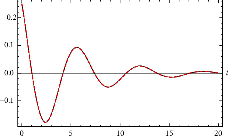
Comparison between the approximate analytical solution and the numerical solution for Example 7.

Example 8 . —

Let

$$\begin{array}{c}\ddot{u}+0.02\dot{u}+u-u^3=0\text{,}\\ u\left(0\right)=0.1\text{\hspace{0.17em}and\hspace{0.17em}}{u}^{\prime }\left(0\right)=0.\end{array}$$ (107)

The error of the approximate analytical solution compared with numerical solution is

$$\begin{array}{c}{\max }_{0\le t\le 150}\left|u_{\text{app}}\left(t\right)-u_{\text{Ruinge}-\text{Kutta}}\left(t\right)\right|=\mathrm{0.00135922.}\end{array}$$ (108)

Comparison between the approximate analytical solution and the numerical solution is shown in Figure 8.

Figure 8.

Comparison between the approximate analytical solution and the numerical solution for Example 8.

Remark 8 . —

Let ρ=ε. An approximate analytical solution to the i.v.p.

$$\begin{array}{c}\ddot{u}+2\epsilon \dot{u}+\alpha u+\beta u^3=0\text{,}\\ u\left(0\right)=u_0\text{\hspace{0.17em}\hspace{0.17em}and\hspace{0.17em}}{u}^{\prime }\left(0\right)=0,\end{array}$$ (109)

is given by

$$\begin{array}{c}u\left(t\right)=\frac{u_0}{1-\left(u_0^2\beta {\epsilon }^2/2{\left(u_0^2\beta +\alpha -{\epsilon }^2\right)}^2\right)sn{\left(f\left(t\right)|m\left(t\right)\right)}^2}\left(cn\left(f\left(t\right)|m\left(t\right)\right)+\frac{\epsilon }{\sqrt{u_0^2\beta +\alpha -{\epsilon }^2}}dn\left(f\left(t\right)|m\left(t\right)\right)sn\left(f\left(t\right)|m\left(t\right)\right)\right)e^{-t\epsilon },\end{array}$$ (110)

where f(t) and m(t) are given by (98) and (99).

5.2. Second Case: u₀=0

Let

$$\begin{array}{c}\ddot{u}+2\epsilon \dot{u}+\alpha u+\beta u^3=0\text{,}u\left(0\right)=0\text{\hspace{0.17em}and\hspace{0.17em}}{u}^{\prime }\left(0\right)={\dot{u}}_0\text{.}\end{array}$$ (111)

Assuming the ansatz [22],

$$\begin{array}{c}u\left(t\right)=-\lambda \sqrt{1-m_0\left(t\right)}\exp \left(-\rho t\right)sd\left(f_0\left(t\right),m_0\left(t\right)\right),\end{array}$$ (112)

we will have

$$\begin{array}{c}{f}_0^{\prime }{\left(t\right)}^2=\frac{1}{2}\beta {\lambda }^2{e}^{-2t\rho }+\kappa ,\end{array}$$ (113)

$$\begin{array}{c}{m}_0\left(t\right)=-\frac{\beta {\lambda }^2}{2f_0^{\prime }{\left(t\right)}^2}{e}^{-2t\rho }.\end{array}$$ (114)

Then,

$$\begin{array}{c}f\left(t\right)=\frac{1}{2\rho }\left(\begin{array}{c}\sqrt{4\kappa +2\beta {\lambda }^2}-\sqrt{4\kappa +2\beta {\lambda }^2{e}^{-2t\rho }}+\\ 2\sqrt{\kappa }{\tanh }^{-1}\left(\sqrt{1+\frac{q{\lambda }^2}{2\kappa }{e}^{-2t\rho }}\right)-2\sqrt{\kappa }{\tanh }^{-1}\left(\sqrt{1+\frac{q{\lambda }^2}{2\kappa }}\right)\end{array}\right),\end{array}$$ (115)

$$\begin{array}{c}m\left(t\right)=-\frac{1}{1+\left(2\kappa /\beta {\lambda }^2\right)e^{2t\rho }}\text{,\hspace{0.17em}}\kappa =p-2\rho \epsilon +{\rho }^2.\end{array}$$ (116)

The number λ is found form the initial condition $u^{\prime }\left(0\right)={\dot{u}}_0$, and its value reads

$$\begin{array}{c}\lambda =-\frac{\sqrt{\left(\sqrt{4{\dot{x}}_0^2\beta +{\left(\alpha -2\epsilon \rho +{\rho }^2\right)}^2}-\alpha +2\epsilon \rho -{\rho }^2/\beta \right)}}{\sqrt{2}}.\end{array}$$ (117)

The number ρ is a solution to some decic equation. Default value is ρ=ε.

Example 9 . —

Let

$$\begin{array}{c}\ddot{u}+0.1\dot{u}+u+u^3=0\text{,}\hspace{1em}u\left(0\right)=0\text{\hspace{0.17em}and\hspace{0.17em}}{u}^{\prime }\left(0\right)=-\mathrm{0.1.}\end{array}$$ (118)

The error of the approximate analytical solution compared with numerical solution is

$$\begin{array}{c}{\max }_{0\le t\le 150}\left|u_{\text{app}}\left(t\right)-u_{\text{Ruinge}-\text{Kutta}}\left(t\right)\right|=\mathrm{0.000303296.}\end{array}$$ (119)

Comparison between the approximate analytical solution and the numerical solution is shown in Figure 9.

Figure 9.

Comparison between the approximate analytical solution and the numerical solution for Example 9.

6. Damped and Forced Duffing Equation

Let us consider the Duffing equation as originally was introduced by Georg Duffing:

$$\begin{array}{c}\ddot{x}+r\dot{x}+{\omega }_0^{2}x+\beta x^3=F\cos \omega t,\end{array}$$ (120)

given the initial conditions

$$\begin{array}{c}x\left(0\right)=x_0\text{\hspace{0.17em}and\hspace{0.17em}}{x}^{\prime }\left(0\right)={\dot{x}}_0.\end{array}$$ (121)

Let

$$\begin{array}{c}x\left(t\right)=u\left(t\right)+c_1\cos \omega t+c_2\sin \omega t.\end{array}$$ (122)

We will suppose that the function u=u(t) is a solution to the Duffing equation

$$\begin{array}{c}\ddot{u}+r\dot{u}+\alpha u+\beta u^3=0\text{,}\\ u\left(0\right)=x_0-c_1\text{\hspace{0.17em}and\hspace{0.17em}}{u}^{\prime }\left(0\right)={\dot{x}}_0-c_2\omega ,\end{array}$$ (123)

where

$$\begin{array}{c}\alpha =\frac{1}{2}\left(3c_1^2\beta +3c_2^2\beta +2{\omega }_0^2\right).\end{array}$$ (124)

The numbers c₁ and c₂ are chosen, so that

$$\begin{array}{c}432F^2{\beta }^3{c}_1^3+1152F{r}^2{\beta }^2{\omega }^2{c}_1^2-192\beta \left(3F^2\beta {\omega }^2-3F^2\beta {\omega }_0^2-4r^4{\omega }^4-4r^2{\omega }^6+8r^2{\omega }_0^2{\omega }^4-4r^2{\omega }_0^4{\omega }^2\right)c_1-192F\beta \left(3F^2\beta -4r^2{\omega }^4+4r^2{\omega }_0^2{\omega }^2\right)=0\end{array}$$ (125)

$$\begin{array}{c}432F^2{\beta }^3{c}_2^3-1152c_2^{2}Fr{\beta }^2\omega \left({\omega }^2-{\omega }_0^2\right)c_2^2+768r^2\beta {\omega }^2\left(r^2{\omega }^2+{\omega }^4-2{\omega }_0^2{\omega }^2+{\omega }_0^4\right)c_2-768F{r}^3\beta {\omega }^3=0.\end{array}$$ (126)

Example 10 . —

Let

$$\begin{array}{c}\ddot{x}+0.1\dot{x}+x+x^3=0.1\cos 0.4t,x\left(0\right)=0\text{\hspace{0.17em}and\hspace{0.17em}}{x}^{\prime }\left(0\right)=0.\end{array}$$ (127)

The error of the approximate analytical solution compared with numerical solution is

$$\begin{array}{c}{\max }_{0\le t\le 150}\left|x_{\text{app}}\left(t\right)-x_{\text{Ruinge}-\text{Kutta}}\left(t\right)\right|=\mathrm{0.00287382.}\end{array}$$ (128)

The approximate solution is

$$\begin{array}{c}x\left(t\right)=e^{-0.05t}\frac{\left(-0.117339\text{cn}-0.00791022\text{dnsn}\right)}{1+1.411\times {10}^{-7}{\text{sn}}^2}+0.00551957\sin \left(0.4t\right)+0.117339\cos \left(0.4t\right),\end{array}$$ (129)

where

$$\begin{array}{c}cn=cn\left(f\left(t\right),m\left(t\right)\right),sn=sn\left(f\left(t\right),m\left(t\right)\right),dn=dn\left(f\left(t\right),m\left(t\right)\right),\\ f\left(t\right)=-20.1343\sqrt{1.0182+0.0137685e^{-0.0993331t}}\\ -5.07916\log \left({\left(1-0.991023\sqrt{1.0182+0.0137685e^{-0.0993331t}}\right)}^2\right)\\ +10.1583\log \left(0.991023\sqrt{1.0182+0.0137685e^{-0.0993331t}}+1\right)-37.4127,\\ m\left(t\right)=\frac{1}{147.903e^{0.0993331t}+2}.\end{array}$$ (130)

Comparison between the approximate analytical solution and the numerical solution is shown in Figure 10.

Finally, let us compare the accuracy of the obtained results in comparation with the homotopy perturbation method (HPM). This method gives the approximate solution:

$$\begin{array}{c}{x}_{\text{HPM}}\left(t\right)=\frac{e^{-\left(1/2\right)t\left(r+\kappa \right)}}{2{\kappa }^2\left(r^2{\omega }^2+{\left({\omega }^2-{\omega }_0^2\right)}^2\right)},\end{array}$$ (131)

$$\begin{array}{c}\left(F\left(r^2\left({\omega }^2-{\omega }_0^2\right)\left(e^{t\kappa }+1\right)-r\kappa \left({\omega }^2+{\omega }_0^2\right)\left(e^{t\kappa }-1\right)+4{\omega }_0^2\left({\omega }_0^2-{\omega }^2\right)\left(e^{t\kappa }+1\right)\right)+2F{\kappa }^2{e}^{\frac{1}{2}t\left(r+\kappa \right)}\left(r\omega \sin \left(t\omega \right)+\left({\omega }_0^2-{\omega }^2\right)\cos \left(t\omega \right)\right)+\left(r^2{\omega }^2+{\left({\omega }^2-{\omega }_0^2\right)}^2\right)\left(x_0\left(r\left(\left(r+\kappa \right)e^{t\kappa }+r-\kappa \right)-4{\omega }_0^2\left(e^{t\kappa }+1\right)\right)+2{\dot{x}}_0\kappa \left(e^{t\kappa }-1\right)\right)\right),\end{array}$$ (132)

$$\begin{array}{c}\kappa =\sqrt{r^2-4{\omega }_0^2}.\end{array}$$ (133)

The error of this approximation compared with numerical solution is

$$\begin{array}{c}{\text{Max}}_{0\le t\le 150}\left|x_{\text{HPM}}\left(t\right)-x_{Ruinge-Kutta}\left(t\right)\right|=\mathrm{0.0136613.}\end{array}$$ (134)

Comparison between the approximate analytical solution and the homotopy solution is shown in Figure 11.

Figure 10.

Comparison between the approximate analytical solution and the numerical solution for Example 10.

Figure 11.

Comparison between the approximate analytical solution and the homotopy solution for Example 10.

7. Analysis and Discussion

We have solved the undamped and constantly forced Duffing equation exactly. Trigonometric approximant was also provided. For the damped or forced case, we derived approximate analytical solution. As far as we know, the Duffing equation (1) has not been solved using the tools we employed in this work. For the damped unforced case, author in [8] obtained approximate analytical solution using generalized Jacobian elliptic functions. More exactly, author considered the following equation:

$$\begin{array}{c}\ddot{x}+2\beta \dot{x}+\alpha x-\epsilon x^3=0\text{,\hspace{0.17em}}x\left(0\right)=x_0\text{\hspace{0.17em}\hspace{0.17em}and\hspace{0.17em}}{x}^{\prime }\left(0\right)={\dot{x}}_0.\end{array}$$ (135)

The obtained solution in [8] has the form

$$\begin{array}{c}x\left(t\right)=c_0\exp \left(-\beta t\right)sn\left(\omega \left(t\right)+c_1,m\left(t\right)\right),\end{array}$$ (136)

where

$$\begin{array}{c}\omega \left(t\right)=\frac{1}{2\beta }\left(\sqrt{2}\left(\sqrt{2\alpha -2{\beta }^2-c_0^2\epsilon }-\sqrt{2\alpha -2{\beta }^2-c_0^2\epsilon e^{-2\beta t}}\right)+2c_0\sqrt{\epsilon }\sqrt{{\beta }^2-\alpha }\left(\frac{\sqrt{1-\left(2\left(\alpha -{\beta }^2\right)/c_0^2\epsilon \right)}{\text{csch}}^{-1}\left(c_0\sqrt{\epsilon }/\sqrt{2{\beta }^2-2\alpha }\right)}{\sqrt{2\alpha -2{\beta }^2-c_0^2\epsilon }}+\frac{e^{\beta t}\sqrt{2\alpha -2{\beta }^2-c_0^2\epsilon e^{-2\beta t}}{\text{csch}}^{-1}\left(c_0\sqrt{\epsilon }{e}^{\beta \left(-t\right)}/\sqrt{2{\beta }^2-2\alpha }\right)}{c_0^2\epsilon \sqrt{\left(2\left({\beta }^2-\alpha \right)e^{2\beta t}/c_0^2\epsilon \right)+1}}\right)\right),\end{array}$$ (137)

$$\begin{array}{c}m\left(t\right)=-\frac{c_0^2\epsilon }{c_0^2\epsilon +2\left({\beta }^2-\alpha \right)e^{2\beta t}}.\end{array}$$ (138)

The constants c₀ and c₁ are determined from the initial conditions as follows:

$$\begin{array}{c}{c}_1=s{n}^{-1}\left(x_0/c_0,m\left(0\right)\right),\end{array}$$ (139)

$$\begin{array}{c}{c}_0=\pm \sqrt{\frac{\alpha }{\epsilon }-\frac{{\beta }^2}{\epsilon }\pm \frac{\sqrt{{\alpha }^2-2\alpha {\beta }^2+{\beta }^4-2\alpha \epsilon x_0^2-4\beta \epsilon x_0{\dot{x}}_0+{\epsilon }^2{x}_0^4-2\epsilon {\dot{x}}_0^2}}{\epsilon }}.\end{array}$$ (140)

This approach is different from the method we used in this work. Let us compare the solution (136) with the solution we obtained in Example 8:

$$\begin{array}{c}\ddot{u}+0.02\dot{u}+u-u^3=0\text{,}u\left(0\right)=0.1\text{\hspace{0.17em}and\hspace{0.17em}}{u}^{\prime }\left(0\right)=0\text{\hspace{0.17em}for\hspace{0.17em}}0\le t\le 150.\end{array}$$ (141)

Using formula gives the approximate analytical solution

$$\begin{array}{c}x\left(t\right)=0.100005e^{-0.01t}sn\left(50.\left(\sqrt{2}\left(1.41767-\sqrt{1.9998+0.010001e^{-0.02t}}\right)-0.2\left(33.4329-\frac{99.9901e^{0.01t}\sqrt{1.9998+0.010001e^{-0.02t}}\csc h^{-1}\left(0.0707177e^{-0.01t}\right)}{\sqrt{1+199.96e^{0.02t}}}\right)\right)+1.55892,\frac{0.010001}{-0.010001-1.9998e^{0.02t}}\right).\end{array}$$ (142)

The error of this solution compared with the Runge–Kutta numerical method equals 0.00142148. The error obtained in our method equals 0.00135922. We may try a simpler ansatz in the form

$$\begin{array}{c}x\left(t\right)=c_0\exp \left(-\rho t\right)\sin \left(w\left(t\right)\right),\end{array}$$ (143)

with

$$\begin{array}{c}w\left(t\right)=\frac{\begin{array}{c}-\sqrt{4\alpha +4\rho \left(\rho -2\beta \right)-3c_0^2\epsilon }+\sqrt{4\alpha +4\rho \left(\rho -2\beta \right)-3c_0^2\epsilon e^{-2\rho t}}+-\sqrt{4\alpha +4\rho \left(\rho -2\beta \right)-3c_0^2\epsilon }+\sqrt{4\alpha +4\rho \left(\rho -2\beta \right)-3c_0^2\epsilon e^{-2\rho t}}+2\sqrt{\alpha +\rho \left(\rho -2\beta \right)}\\ \left({\text{coth}}^{-1}\left(\left(2\sqrt{\alpha +\rho \left(\rho -2\beta \right)}/\sqrt{4\alpha +4\rho \left(\rho -2\beta \right)-3c_0^2\epsilon }\right)\right)-{\text{coth}}^{-1}\left(\left(2\sqrt{\alpha +\rho \left(\rho -2\beta \right)}/\sqrt{4\alpha +4\rho \left(\rho -2\beta \right)-3c_0^2\epsilon e^{-2\rho t}}\right)\right)\right)\end{array}}{2\rho }.\end{array}$$ (144)

The numbers c₀ and ρ are determined from the system

$$\begin{array}{c}-8\alpha \beta +8\alpha \rho +16{\beta }^2\rho -24\beta {\rho }^2+6\beta c_0^2\epsilon -9c_0^2\epsilon \rho +8{\rho }^3=0,\\ -4\alpha c_0^2+8\beta c_0^2\rho +3\beta c_0^4\epsilon -4c_0^2{\rho }^2-3c_0^2\epsilon x_0^2+4\alpha x_0^2+8\beta \rho x_0^2+8{\rho }^2{x}_0^2+8\rho x_0{\dot{x}}_o+4{\dot{x}}_0^2=0.\end{array}$$ (145)

Using this ansatz, we obtain the approximate analytical solution:

$$\begin{array}{c}{x}_{\text{trigo}}\left(t\right)=0.100005e^{-0.00996291t}\\ \sin \left(1.56087+50.1861\left(\sqrt{3.9996+0.030003e^{-0.0199258t}}+1.9999\left(-{\text{coth}}^{-1}\left(\frac{1.9999}{\sqrt{3.9996+0.030003e^{-0.0199258t}}}\right)+\left(3.14134-1.5708i\right)\right)-2.00739\right)\right)\end{array}$$ (146)

The error of the trigonometric solution (146) compared with the numerical solution using the Runge–Kutta method equals 0.00195254, so that the trigonometric solution is good as well.

8. Conclusions and Future Work

The methods employed here may be useful to study other nonlinear oscillators of the form

$$\begin{array}{c}\ddot{x}+2\delta \dot{x}+f\left(x\right)=F\cos \omega t,x\left(0\right)=x_0\text{\hspace{0.17em}and\hspace{0.17em}}{x}^{\prime }\left(0\right)={\dot{x}}_0,\end{array}$$ (147)

where the function f is odd: f(−x)=−f(x). To this end, we approximate this function on some interval [−A, A] by means of Chebyshev polynomials in the form

$$\begin{array}{c}f\left(x\right)\approx px+q{x}^3.\end{array}$$ (148)

Then, the i.v.p. is replaced with the i.v.p.

$$\begin{array}{c}\ddot{x}+2\delta \dot{x}+px+q{x}^3=F\cos \omega t,x\left(0\right)=x_0\text{\hspace{0.17em}and\hspace{0.17em}}{x}^{\prime }\left(0\right)={\dot{x}}_0.\end{array}$$ (149)

On the other hand, we may study the following cubic quintic Duffing oscillator:

$$\begin{array}{c}\ddot{x}+2\delta \dot{x}+px+q{x}^3+r{x}^5=F\cos \omega t,x\left(0\right)=x_0\text{\hspace{0.17em}and\hspace{0.17em}}{x}^{\prime }\left(0\right)={\dot{x}}_0.\end{array}$$ (150)

For the unforced and damped cases, we may try the ansatz

$$\begin{array}{c}x\left(t\right)=c_0\exp \left(-\rho t\right)\sin \left(f\left(t\right)+\text{arccos}\left(\frac{x_0}{c_0}\right)\right),\end{array}$$ (151)

where

$$\begin{array}{c}f\left(t\right)=\frac{1}{2\sqrt{2}}{\displaystyle {\int }_0^t\sqrt{8p-16\delta \rho +8{\rho }^2+6c_0^2{e}^{-2\tau \rho }q+5c_0^4{e}^{-4\tau \rho }r}}\text{d}\tau ,\end{array}$$ (152)

and

$$\begin{array}{c}8\left(p{x}_0^2-2\delta \rho x_0^2+2{\rho }^2{x}_0^2+2\rho {\dot{x}}_0{x}_0+{\dot{x}}_0^2\right)-2\left(-8\delta \rho +4p+4{\rho }^2-3q{x}_0^2\right)c_0^2+\left(5r{x}_0^2-6q\right)c_0^4-5r{c}_0^6=0.\end{array}$$ (153)

The number ρ is a free parameter that is chosen in order to minimize the residual error

Data Availability

No data were used to support this study.

Conflicts of Interest

The authors declare that they have no conflicts of interest.

References

- 1.Duffing G. Erzwungene Schwingung bei veränderlicher Eigenfrequenz und ihre technische Bedeutung . Braunschweig, Germany: Vieweg; 1918. [Google Scholar]
- 2.Feng Z. A qualitative study of the damped duffing equation andApplications. Discrete and continuous dynamical systems-series B. Follow journal . 5(5) doi: 10.3934/dcdsb.2006.6.1097. [DOI] [Google Scholar]
- 3.Loria A., Panteley E., Nijmeijer H. Control of the chaotic Duffing equation withuncertainty in all parameters. IEEE Transactions on Circuits and Systems I . 1998;45(12):1252–1255. doi: 10.1109/81.736558. [DOI] [Google Scholar]
- 4.Thompson J. M. T., Stewart H. B. Nonlinear Dynamics and Chaos . New York, NY, USA: John Wiley & Sons; 1986. [Google Scholar]
- 5.Moon F. C. Chaotic Vibrations: An Introduction for Applied Scientists and Engineers . New York, NY, USA: John Wiley & Sons; 1987. [Google Scholar]
- 6.Dowell E. H., Pezeshki C. On the understanding of chaos in Duffing’s equation in-cluding a comparison with experiment. Journal of Applied Mechanics . 1986;53(1):5–9. doi: 10.1115/1.3171739. [DOI] [Google Scholar]
- 7.Battelli F., Palmer K. J. Chaos in the duffing equation. Journal of Differential Equations . 1993;101(2):276–301. doi: 10.1006/jdeq.1993.1013. [DOI] [Google Scholar]
- 8.Johannesen K. The duffing oscillator equation and its applications in physics. European Journal of Physics . 2015;36065020 [Google Scholar]
- 9.Johannesen K. International Journal of Applied and Computational Mathematics . 2017;3:p. 3805. [Google Scholar]
- 10.He Ji-H., Yusry O., El-Dib A tutorial introduction to the two-scale fractal calculus and its application to the fractal zhiber-shabat oscillator. Fractals . 2021;29 doi: 10.1142/S0218348X21502686. [DOI] [Google Scholar]
- 11.He J. H., Nurakhmetov D., Skrzypacz P., Wei D. M. Dynamic pull-in for micro-electromechanical device with a current-carrying conductor. Journal of Low Frequency Noise, Vibration and Active Control . 2021;40(2):1059–1066. doi: 10.1177/1461348419847298. [DOI] [Google Scholar]
- 12.He J.-H., Amer T. S., Elnaggar S., Galal A. A. Periodic property and instability of a rotating pendulum system. Axioms . 2021;10(3):p. 191. doi: 10.3390/axioms10030191. [DOI] [Google Scholar]
- 13.He J.-H., Yang Q., He C.-H., Khan Y. A simple frequency formulation for the tangent oscillator. Axioms . 2021;10(4):p. 320. doi: 10.3390/axioms10040320. [DOI] [Google Scholar]
- 14.Tian D., Ain Q. T., Anjum N., He C. H., Cheng B. Fractal N/MEMS: from pull-in instability to pull-in stability. Fractals . 2021;29(2) doi: 10.1142/s0218348x21500304.2150030 [DOI] [Google Scholar]
- 15.Tian D., He C. H. A fractal micro-electromechanical system and its pull-in stability. Journal of Low Frequency Noise, Vibration and Active Control . 2021;40(3):1380–1386. doi: 10.1177/1461348420984041. [DOI] [Google Scholar]
- 16.He C. H., Tian D., Moatimid G. M., Salman H. F., Zekry M. H. Hybrid Rayleigh–van der pol–duffing oscillator: stability analysis and controller. Journal of Low Frequency Noise, Vibration and Active Control . 2021;41(1):244–268. doi: 10.1177/14613484211026407. [DOI] [Google Scholar]
- 17.He C.-H., El-Dib Y. O. A heuristic review on the homotopy perturbation method for non-conservative oscillators. Journal of Low Frequency Noise, Vibration and Active Control . 2021 doi: 10.1177/14613484211059264.146134842110592 [DOI] [Google Scholar]
- 18.NaumanAhmed. Structure preserving numerical analysis of hiv and cd4+t-cells reaction diffusion model in two space dimensions, chaos. Solitons & Fractals . 2020;139 [Google Scholar]
- 19.Malik M. R. Design and stability analysis of a nonlinear SEIQR infectious model and its efficient non-local computational implementation. Applied Mathematical Modelling . 2021;89(2):1835–1846. doi: 10.1016/j.apm.2020.08.082. [DOI] [PMC free article] [PubMed] [Google Scholar]
- 20.Salas A. H. The duffing oscillator equation and its applications in physics. Mathematical Problems in Engineering . 2021;2021:13. doi: 10.1155/2021/9994967. https://www.hindawi.com/journals/mpe/2021/9994967/ 9994967 [DOI] [Google Scholar]
- 21.Salas A. H. Analytic solution to the generalized complex Duffing equation and its application in soliton theory. Applicable Analysis . 100 doi: 10.1080/00036811.2019.1698729. [DOI] [Google Scholar]
- 22.Salas A. H., El-Tantawy S. A. On the approximate solutions to a damped harmonic oscillator with higher-order nonlinearities and its application to plasma physics: semi-analytical solution and moving boundary method. European Physical Journal . 2020;135(10):833–917. doi: 10.1140/epjp/s13360-020-00829-3. [DOI] [Google Scholar]
Associated Data
This section collects any data citations, data availability statements, or supplementary materials included in this article.
Data Availability Statement