A primer on dose-response data modeling in radiotherapy

Abstract

An overview of common approaches used to assess for a dose-response for RT-associated endpoints is presented, using lung toxicity data sets analyzed as a part of the HyTEC effort as an example. Each component presented (e.g., data-driven analysis, dose-response analysis, and calculating uncertainties on model prediction) is addressed using established approaches. Specifically, the maximum likelihood method was used to calculate best parameter values of the commonly used logistic model, the profile-likelihood to calculate confidence intervals on model parameters, and the likelihood ratio to determine if the observed data fit is statistically significant. The bootstrap method was used to calculate confidence intervals for model predictions. Correlated behavior of model parameters and implication for interpreting dose-response are discussed.

Short Summary

An overview of common approaches used to assess for a dose-response for RT-associated endpoints is presented. Specific components of data-driven analysis and dose-response modeling are described. Specifically, methods to calculate best parameter values and confidence intervals, to determine if the observed data fit is statistically significant, to calculate confidence intervals for model predictions and to account for correlated behavior of model parameters are presented. Implications for interpreting dose-response in clinical practice are discussed.

Introduction

The broad goals of the HyTEC effort were to summarize/model published data on dose-volume-response for both normal tissues and tumors of hypofractionation regimens to provide guidance for radiotherapy planning. Deriving dose/volume/outcome guidance from clinical information is commonly achieved via data analyses alone (e.g., comparing dose/volume parameters in patients with toxicity vs. without toxicity), or by dose-response modeling (e.g., assessing the correlation between the incidence of complications vs. dose/volume parameters). The latter approach allows for prediction of the risk of complication for a new patient and also provides the opportunity to set constraints based upon a clinically-acceptable complication rates when new treatments are designed.

We herein describe a step-by-step process of dose-response analysis via commonly used methods (1) to illustrate the specific goals achieved in each step, associated pitfalls, and the interpretation of the results. Routine use of dose-response models to guide planning optimization objectives implies a “dependence” that may not exist, even if statistical tests may show significance. Therefore, caution should be followed when applying these methods clinically. Our goal is to provide an overview of the different components of dose-response analysis for use in radiotherapy planning that are typically not discussed but assumed in the published literature, a look under the hood so to speak. There are potential pitfalls in fitting a model to clinical data, and we explore some of these here. We specifically emphasize correlated behavior of model parameters and the impact of this behavior on the calculated confidence intervals. The audience for this review includes individuals who want to perform or understand more deeply outcome (TCP/NTCP) modelling, and we have tried to highlight the clinical importance of these concepts/methods for the clinician-reader.

Model Selection

Various models have been used to describe dose-response relationships. Within the range of available data, the differences between the predictions from different models will typically be modest. Beyond the range of available data, inter-model differences in predictions will typically be larger (2,3), and thus model selection is particularly impactful when making extrapolations. For example, the type of model chosen (e.g., logistic, log-logistic or probit) determines the generic shape of the assumed dose-response relationship and can dramatically impact such extrapolations. In addition, even for the same model type, predictions will be driven by parameter values, and these are sensitive to how the data fitting was performed (e.g., maximum likelihood vs. least squares (2)).

Maximum likelihood estimation (MLE) is a standard widely-adopted data-fitting approach (1,4,5) that aims to capture the most frequent patterns in the data (and hence the name) and can overcome some of the noisy variations that are associated with deterministic methods such as least squares. This is specifically important in radiotherapy dose-response models based on retrospective data, where the data may not be of the highest quality and subject to fluctuations due to contour or treatment planning variability or human subjectivity. The maximum likelihood method directly incorporates the number of patients in each dose or dose-volume group. Therefore, the model is driven towards agreement with the data in the most “populated” range and is not overly sensitive to occasional outliers. In contrast, model parameter fitting using least squares is sensitive to the “poorly populated” data points. Modification to this method can be made by assigning a weight to each data point. However, as Bentzen and Tucker astutely stated: “if this information is available, then MLE is to be preferred anyway” (2).

Regardless of the model type, fitting method, or software used for fitting the model, the basic principles remain the same. Model parameters (and their confidence intervals) must be calculated, significance of dose-response has to be tested, and confidence intervals on model predictions should be established. These three components are inter-dependent, and uncertainties in one propagate to another—thus, results obtained in each component of fitting for dose-response must be interpreted with care.

Example exploratory analysis of a clinical data set

Combined data from two papers (6,7) provided the material for this exercise. Radiation-induced pneumonitis (RP), Grade 2 or higher, was used as the clinical endpoint. Possible dependence of incidence of RP on mean lung dose (MLD) was explored. Statistical analysis of the source data was performed using the Statistica software (Statsoft, Tulsa, OK). Fitting for dose-response was performed with an in-house computer code cross-validated by multiple contributors to the HyTEC effort (8-10).

Exploratory visual inspection, e.g., scatter plots, followed by simple descriptive statistical tests are good starting points to evaluate whether finding a dose-response is an attainable goal. Commonly, data are displayed as patient-specific plots with each patient classified as exhibiting toxicity, or not (Figure 1).

Figure 1.

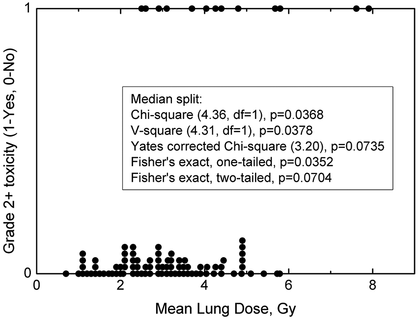
Patient mean lung dose (MLD) and toxicity summary, where each point represents an individual patient exhibiting toxicity labelled as “1”, or without toxicity labelled as “0”. Overlapping or near-overlapping points (same or similar MLD) have been incremented by 0.025 to show the number of patients receiving particular MLD. Insert shows basic description statistics with a median MLD split. df = degrees of freedom. Median MLD is 3.05 Gy.

While this representation of the data—one point=one patient— provides only a qualitative impression, it can be quite informative. We can readily assess the MLD range, number of events (toxicities), and possibly their distribution, specifically whether more toxicity events are tail heavy towards larger MLD or not. Visually the data may look promising: the number of patients is robust, there are 13 toxicities giving an event rate of 13/96 (13.5%), and the proportion of events seem to be dependent on increased MLD.

As a general rule of thumb, the number of events (toxicities) is recommended to be at least 10 for each model parameter. In a two parameter logistic regression (the MLD₅₀ and the slope, described in detail below) at least 20 events are desired (11). If the number of events per variable is less than 10, parameter estimates may be biased and likelihood of paradoxical associations, i.e., significance in the wrong direction, may increase. However, a smaller number may suffice, if there is a definitive correlation, depending on the exact situation. A simple approach to assess for a signal is to divide the group at the median MLD (12) into two halves (termed ‘median split’) and perform a descriptive statistics tests on the two groups (i.e., compare the rate of RP in the upper (top 50 percentile) vs lower groups (bottom 50 percentile)). This method is not intended to search for the best cut-point. More sophisticated data-driven approaches, including receiver operating characteristics (ROC) analysis governed by sensitivity and specificity have been used. Cut point can be optimally determined from the Youden index of the ROC curve (13). Also, tests to check how the data, e.g., MLD, are distributed among toxicity vs no toxicity patientscan be performed.

As shown in the Figure 1 legend, several simple statistical tests on RP incidences for the two groups (above vs. below the median value 3.05 Gy) suggest a possible “signal”, i.e., dose-response. This median splits analysis has been used in the literature as a means to test for predictive power of a parameter in question (12). However, due to its simplicity, the median split does not substitute for full regression analysis. Median splits only suggest if there is a relationship between dose and the endpoint but not what that relationship may look like.

Our judgement of whether patients with larger MLD are more likely to develop grade 2+ RP—and whether the difference is significant—would ultimately depend on the statistical test chosen. In this example, the p-values ranged from <0.05 (for several options shown in Figure 1 legend) to marginal significance with a p=0.070 with the Fisher’s exact two-tailed test. Some statistical tests may not be appropriate in this setting (e.g., non-parametric approaches such as the Wilcoxon rank sum where independence and variance equivalency need to be evaluated before application). If not checked beforehand, the test may yield fortuitous results such as yielding a highly significant association of p=0.002. Modelers and clinician consumers of these models need to be cognizant of these subtleties and the main underlying assumptions of the different statistical tests. Typically, more informed/sophisticated dose-response analyses are needed for our TCP and NTCP models.

Sigmoidal dose-response: model parameters and confidence intervals

Dose-response data are most commonly assumed to follow a sigmoid-shaped function. Popular choices to describe this dependency are logistic, log-logistic and probit (14). Details are shown in Supplement A. The logistic model was used in this report:

$$P(X\mid X_{50},{\gamma }_{50})=\frac{1}{1+\text{exp}[-4{\gamma }_{50}(\frac{X}{X_{50}}-1)]}$$ (1)

where P(X∣X₅₀,γ₅₀) is the probability of response, X is the variable of interest (in this case MLD). Notation ∣X₅₀,γ₅₀ means that the probability of response in calculated given model parameters are X₅₀, at which 50% of patients show response, and the slope parameter γ₅₀. Here, X₅₀=MLD₅₀, but in the other scenario it can certainly be other dose-based metrics such as maximum dose, median dose, minimum dose to the hottest volume v, D_v, or equivalent uniform dose, EUD (all at the 50% risk level). The normalized dose-response gradient γ₅₀=X₅₀ρP(X)/ρX, is proportional to the slope of the curve at the 50% value and represents change in response expressed relative to change in X relative to X₅₀. For example, a γ₅₀=2 means that for each 1% change in X at X₅₀ there is a 2-percentage point change in response.

This assumption that the data follow a sigmoid-shaped function ranging from 0% to 100% incidence at does not always hold. For example, incidence of liver toxicity has been reported to not reach 0% even of mean liver dose is 0 Gy due to residual disease (15). To only account for radiation-induced toxicity an offset to the model can be introduced (16). Conversely, in the HyTEC effort with V_x (volume of normal tissue receiving at least dose x) serving as an independent variable, logarithm of Vx as opposed to V_x was used in some of the models. This avoids prediction of non-zero probability of response, e.g., toxicity, for V_x=0 (17).

Machine learning algorithms to predict response to therapy have been gaining popularity, for example when radiomics-based prediction models are developed (18). This paper is focused on parametric models, where the shape of the response is assumed to follow a commonly assumed sigmoidal shape. When non-parametric methods are used the shape of the response is unknown and is captured from the data. Given the larger degrees of freedom these methods tend to perform generally better in terms of predictive power, but with limited underlying understanding of response shape (19).

The considered logistic model describes probability of response as a function of a single metric, MLD. More sophisticated models have been developed to account for the partial volume effect, i.e., relationship between tissue tolerance and the treated volume. Two examples are: the Lyman-Kutcher-Burman (LKB) probit-based model (20,21) and the Poisson-based relative seriality model (22). These models contain a parameter describing the strength of the volume effect, n in the LKB, and s in the relative seriality model. Values of these parameters show if the organ/response is serial, which means incidence of toxicity depends on hot spots (small volumes receiving near maximum dose), or parallel, incidence of toxicity is dependent on mean dose, or anything in between. If organ/response is serial n→0 and s→1, conversely for a parallel organ/response n→1 and s→0. Both models have been used to analyze SBRT outcomes data, for example carotid blowout (23).

While LKB and relative seriality models are meant to be used for an organ or tissue with any architecture, for specific tissue/organ functional subunit arrangements, alternative approaches have been proposed. For example, the parallel model (24) has been developed for ‘parallel arranged’ organs, which can tolerate high doses to small volumes, e.g., lung or liver. Critical element models (25,26) are primarily intended for ‘serially arranged’ organs where damage to a small region can lead to a complication, e.g., optic nerve or spinal cord. Describing probability of toxicity as a function of one metric has a practical advantage that incidence-driven guidelines can be derived for the dose-volume metrics of choice. For example, in the HyTEC effort mean dose has been used for liver (9), and maximum dose for optic pathways (27). Sparsity of data, heterogeneity of data, and limited reporting of details, are three good reasons why simple logistic models are a good starting point to test for correlations and produce evidence-driven guidelines following the parsimony principle of data analytics. In the clinical setting sparing organs sensitive to hots spots is challenging. The data we have seen thus far indicate that very small volumes determine much of the outcomes for SBRT, so we often used logistic or probit models on very small DVH cutpoints like D0.1cc or D0.03cc. Pooled data rarely reflect access to full DVH data, therefore accounting for volume effect is not feasible at present. Use of more sophisticated models such as LKB or relative seriality would be a great future topic when we can access full DVH datasets. The functions themselves do not have any radiobiological content aside from the fact that the probability of the endpoint goes from zero at one extreme to 100% at the other.

When data from the literature are pooled together, as was the case in the HyTEC effort, commonality in the data used in the model is required. In particular, the number of fractions may vary from a single to as many as 10. Converting doses into the equivalent dose in 2 Gy fractions (EQD2) has been commonly used (8,27). Because conversion of MLD to mean EQD2 is non-linear it cannot be performed without full DVH data. This puts a limitation on synthesizing the data and reporting both physical dose and EQD2 is encouraged.

The search for the model parameters that best fit the data was performed using the maximum likelihood method (1,4), where each patient’s outcome is scored binary as Yes vs. No for pneumonitis. For continuous outcomes (e.g., % reduction in pulmonary function relative to pre-RT baseline), outcome data are commonly dichotomized (e.g., above vs. below a certain degree of reduction).

In the most general sense, consider a study, with a variable of interest taking values X_i. The number of patients whose variable of interest equals X_i is n_i, and r_i is the number of responders (in our example, one might consider there to be n_i patients with an X_i [MLD = some value], and r_i of these get pneumonitis). In toxicity studies, finding two or more patients with exactly the same MLD is virtually impossible, therefore X_i can be viewed as a middle of an MLD bin. In tumor control probability (TCP) studies the prescribed dose can be designated as X_i and naturally there will be many patients treated with this prescription. The model under consideration predicts probability of response, given model parameters X₅₀ and γ₅₀ and the variable value X, P(X∣X₅₀,γ₅₀). Log-likelihood of the observed outcome, LL, given model predictions is:

$$LL=\sum [r_i\text{ln}\left(P(X_i\mid X_{50},{\gamma }_{50})\right)+(n_i-r_i)\text{ln}\left(1-P(X_i\mid X_{50},{\gamma }_{50})\right)]$$ (2)

The LL function searches through the possible range of values for X₅₀, and γ₅₀, to find the combination of parameter values that best describes the observed outcome (i.e., maximizing the value of the LL function, hence the term maximum likelihood method). Once these “optimal” parameter values are determined, the dose-response curve can be plotted (see Figure 2 for our example, with reference parameter values shown in the insert). The observed actual clinical data are also shown, but, in contrast with Figure 1 patients were grouped into smaller bins based on ranges of MLD (with bin sizes/ranges defined either by MLD ranges or bin sizes). The exact manner that the clinical data are binned for this display is not critical, as the intent is to broadly/subjectively assess the degree to which the model-based predictions fit the observed data. The model-based curve was derived from the clinical data, that statistical linkage was already defined by the LL function noted above. At this point, we are merely circling back to assess/verify this fit.

Figure 2.

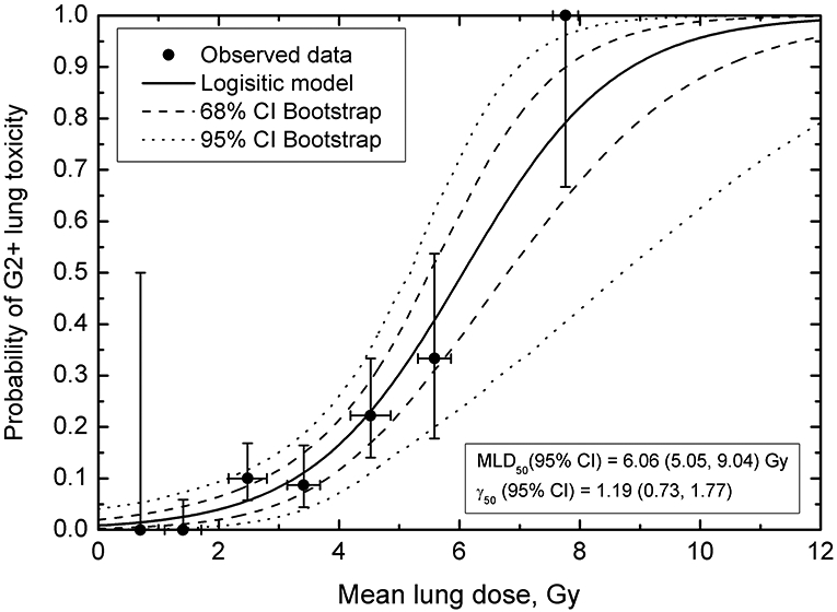
Probability of Grade 2 or higher toxicity as a function of mean lung dose. Horizontal error bars on data points are standard deviation for MLD for patients in a particular MLD bin; vertical error bars are 68% binomial CI for the observed outcome. Solid line shows the logistic curve, dashed and dotted lines are confidence intervals calculated using bootstrap (68% dashed, 95% dotted). Bin size was set to 1 Gy to obtain sufficient resolution to visualize MLD-response while keeping MLD variance within the bin reasonably small.

Maximum-likelihood method assigns “weight” to each data point in Figure 2 according to the number of patients in the dose group. Therefore, calculated model parameter values best fitting the observed data are not overly sensitive to poorly populated data points. For example, if the 100% incidence data point near MLD=8 Gy (two patients, both showed toxicity) was removed from fitting, model parameter values would have been MLD₅₀=6.58 Gy and γ₅₀=1.07. This is well within confidence intervals obtained for the full data set, Figure 2. The number of patients in each group and overall distribution of data points in terms of MLD and incidence will have implications for confidence intervals calculated for the model predictions, see below. The question of data sufficiency is complex. The success in building a dose-response model will depend on numerous factors, specifically variation in the explored dose or dose-volume variable, number of patients in the study, number of observed events, variation in incidence, possible impact of non-dosimetric factors. Data-driven approaches shown above are an early indicators if dose-response model can be built.

This depiction of the observed data, with patients grouped into MLD bins (Figure 2), is convenient for visualization and for estimating input data uncertainties. Observed incidence of toxicity as a function of MLD is shown, something that is not apparent in Figure 1, and vertical error bars show if a particular point carries a lot or a little weight, i.e., how many patients belong to this MLD bin. The horizontal error bars denote standard deviations for MLD for patients in an MLD bin. When model parameters best fitting the observed data are calculated, LL values are calculated for a broad range of parameter values in search for a maximum LL value, equation (2). Whenever individual data are available, patients are entered into equation (2) one at a time (24). Therefore n_i=1, and r_i is either equal 1 (toxicity=Yes) or 0 (toxicity=No). This is a best case scenario when individual data were presented or shared by the authors. In the HyTEC effort, this was not always possible as we were limited by what was published.

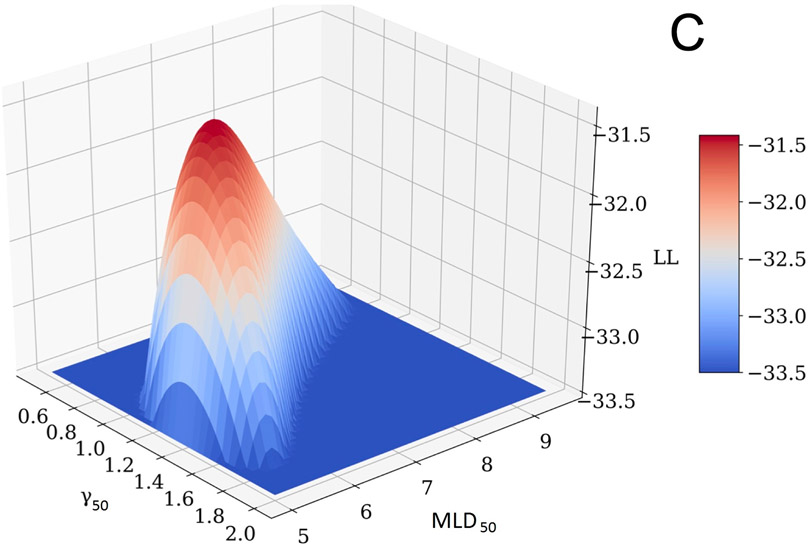
The profile-likelihood method was used to calculate 95% CI for the model parameters (Figure 3, panels A and B). To calculate these CIs, the LL profile was searched for MLD₅₀ and γ₅₀ values where the LL function value drops below its maximum (MLL) value of −31.41 minus 1.92, which is a chi-square for 1 degree of freedom, 3.84, divided by 2 (1,4). If a model has two parameters, as in this case, LL is a surface which behaves like a mountain top, panel C. The search for parameter CI can be visualized as a profile of a projection to one of the planes. Specifically, the profile of MLD₅₀ shown in panel A is a projection of the surface in panel C on the MLD₅₀-LL plane; and the profile of γ₅₀, panel B is a projection of the surface, panel C, on the γ₅₀-LL plane. A critical point here—and where calculations can go awry—is that when the LL value in the profile is calculated for a particular value of one parameter (say, MLD₅₀) then the LL value to be used in profile-likelihood is the maximum value for this MLD₅₀ and ANY γ₅₀. Notice that profile-likelihood method can capture the asymmetry in CI in contrast with normal approximations, which tend to be symmetric. MLD₅₀ and γ₅₀ values providing the best fit to the observed data correspond to the global maximum of −31.41, shown in Figure 3.

Figure 3.

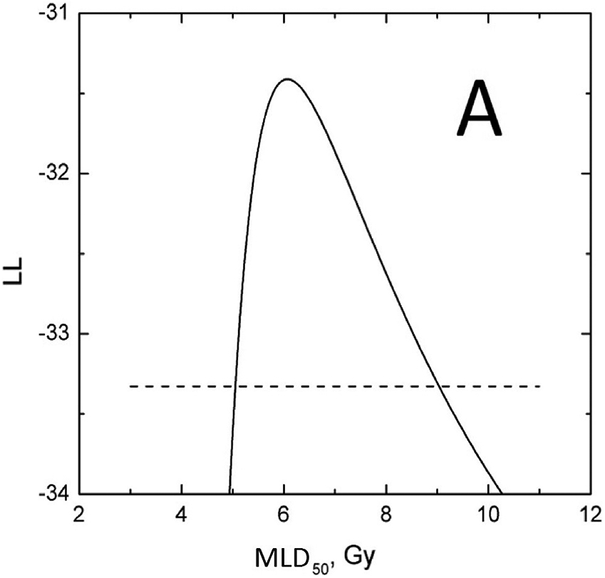
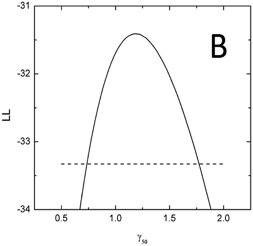
D₅₀ (panel A) and γ₅₀ (panel B) LL profiles to calculate the parameter value CIs. Horizontal dashed line is a cut-off which is maximum LL, −31.41 minus 1.92. Profiles maximize at best values. Panel C shows a LL surface as a function of D₅₀ and γ₅₀. Profiles in panels A and B are projections of the surface onto D₅₀-LL and γ₅₀-LL planes. For any MLD₅₀ value in panel A, γ₅₀ is selected so that LL takes the maximum value for the considered MLD₅₀, and vice versa for panel B.

Determining the significance of dose-response

The calculation of model parameters that best fit the data and plotting a sigmoidal-shaped function as shown in Figure 2, does not signify a meaningful relationship, i.e., incidence of pneumonitis increases as MLD increases. In statistical terms, the question is whether we can reject the null hypothesis that the incidence of an outcome as a function of the parameter under consideration (in this case pneumonitis risk vs. MLD) show no relationship.

CIs calculated for model parameters are revealing; specifically, the lower CI for the normalized slope is >0. This, however, does not tell us about the level of significance of this dose-response and the extent to which the model’s dose-response is an improvement compared to no relationship assumed under null hypothesis. Because this null hypothesis assumes no relationship, e.g., as MLD increases incidence of pneumonitis does not change, it can be visualized as a horizontal line through the probability averaged over all patients and LL can be calculated for this hypothesis. The likelihood ratio test comparing MLL of the model against LL for the average probability of response, can be used to test if the model significantly improves on the null hypothesis, i.e., horizontal line fit. The average probability is the total number of responders, r, divided by the total number of patients, n:

$$P_{ave}=\frac{\sum r_i}{\sum n_i}=\frac{r}{n}$$ (3)

LL for this value, LL(P_ave):

$$LL(P_{ave})=\text{ln}(P_{ave})\sum r_i+\text{ln}(1-P_{ave})(\sum n_i-\sum r_i)$$ (4)

Which can be also written as:

$$LL(r,n)=\text{rln}(r∕n)+(\mathrm{n}-\mathrm{r})\text{ln}((n-r)∕n)$$ (5)

If the difference between LL values, MLL-LL(P_ave) is larger than 1.92, the improvement in LL as a measure of goodness of fit, logistic model vs. assumed no relationship, is statistically significant. In this example, MLL is −31.41, LL(P_ave)=−38.07, giving us a difference of 6.66 (p=0.0003), and hence we can reject the null hypothesis and conclude that probability of pneumonitis increases as MLD increases.

In clinical practice, the question is whether the model can be reliably applied to patients. Calculating sensitivity, specificity and related descriptors, e.g., negative predictive value (NPV), may provide further needed perspective. High value of NPV, which is the proportion of patients, %, who do not show complications when the guideline is fulfilled (the number of true negatives over the total of true plus false negatives), would support the validity of a guideline. . For example, if incidence of toxicity of 10% is set as clinically acceptable (MLD=3.27 Gy), NPV for MLD<3.27 Gy is 52/56=92.9%. The model thereby allows us to evaluate clinical protocols and formulate planning objectives.

Model parameters: correlated behavior (i.e., interplay)

The above steps provide answers to the most commonly asked questions: data have been tested for correlation between the outcomes (toxicity) and the variable of choice (MLD), model parameters and confidence intervals have been calculated, and the statistical significance for the observed dependence has been established. Typically, a dose-response curve calculated for the obtained model parameters, e.g. MLD₅₀ and γ₅₀, is presented in the literature. Confidence intervals for the calculated response probability ideally need to be presented. However, direct use of CI on model parameters in an uncoupled manner ignores the interplay between MLD₅₀ and γ₅₀.

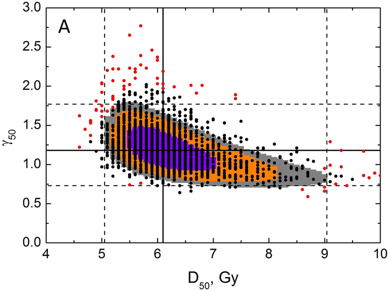
Specifically, Figure 3, panels A and B, which show the LL profiles, are simply a projection of a 3D LL surface to a plane and ignore the shape of the surface shown in panel C. Figure 4, panel A shows LL areas which can be visualized as planar cuts through the LL surface (Figure 3C). Model parameter values best fitting the data (solid lines) and CI (dashed lines) are shown in Figure 4A. It would be incorrect to assume that if the CI for D₅₀ is 5.05-9.04 and for γ₅₀ is 0.73-1.77, then the rectangle formed by intersection of these CI (dashed lines Figure 4A) would signify the area for all possible combinations of D₅₀ and γ₅₀ belonging to the combined CI. The underlying assumption would be uncoupled behavior of these parameters.

Figure 4.

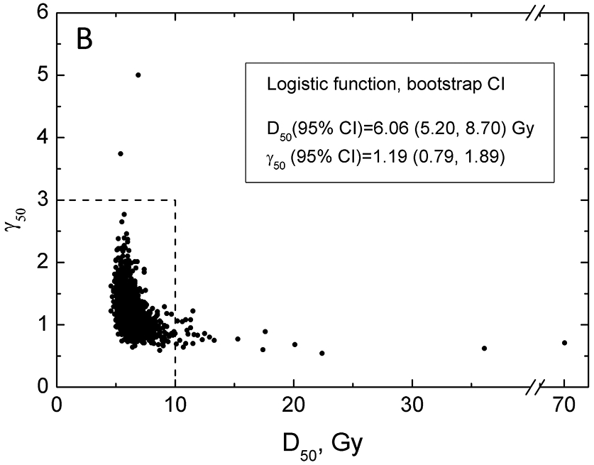
Results of bootstrap analysis. Each point is D₅₀ and γ₅₀ calculated for a sample of patient obtained by random sampling with replacement, 2000 histories were ran. Panel A: Zoomed-in view showing a restricted range of D50 and γ₅₀. LL areas calculated as MLL minus 0.495 (violet), 1.353 (orange) and 1.92 (grey), which are chi-square values for 1 degree of freedom divided by 2 for p=0.68, 0.90 and 0.95. Model parameter values best fitting the data are shown as black solid line, dashed lines are 95% CIs for the model parameters. The 100 red points reflect the 5% of the data which contribute the least to the CI within the MLD range 0-12Gy. Panel B: Zoomed-out view, with wider range of D50 and γ₅₀ (dotted lines reflect the data range in panel A), with full results of bootstrap analysis. The legend shows CI for model parameters calculated using bootstrap.

Careful inspection of the LL surface in Figure 3C shows that D₅₀ and γ₅₀ profiles are not bell-shaped but rather asymmetric. This demonstrates the interplay between D₅₀ and γ₅₀. This correlated behavior is further demonstrated by planar cuts through the LL surface, Figure 4A. The figure shows that iso LL lines take a banana-like shape where a larger D₅₀ requires a shallower slope to maintain LL. This figure further demonstrates implication for CI and best value for the model parameters superimposed on the iso-LL lines. A mathematical overview explaining correlated behavior of model parameters is shown in the Supplement B.

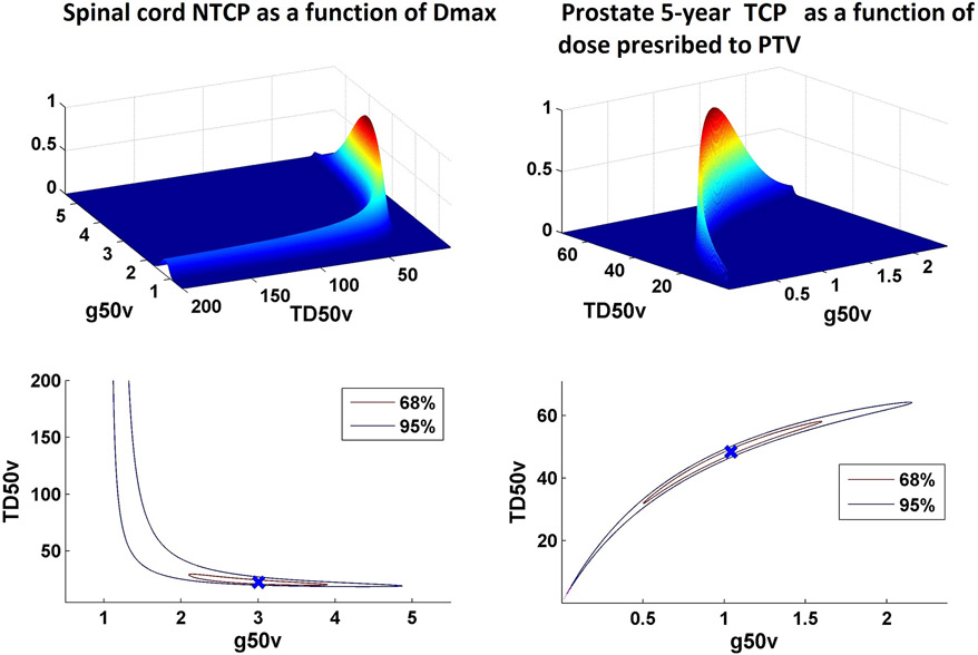
For the data set considered here for lung, the “degree of banananess” is modest, as the data covers a broad range of incidence of complications. However, in other situations, in particular when data are limited to either high or low probability ranges, this correlated behavior of model parameters may lead to iso-LL areas occupying narrow bands thereby leading to an “extreme banana” shape. Figure 5 shows examples of this behavior for spinal cord tolerance (where the incidence of complication is extremely low) and prostate TCP (where the control rate is high) from the HyTEC papers (28). In these situations, where bulk of the clinical data resides far from D₅₀, calculated TCP/NTCP values become sensitive to small uncertainties in γ₅₀. Therefore, convergence criteria to calculate γ₅₀ have to be tight and rounding has to be avoided as this impact calculated values. The excessive number of decimal places for the γ₅₀ do not imply significant figures but are needed for reproducibility because most of the data is far from 50% response where γ₅₀ is defined.

Figure 5.

Relationship of TD50 and slope parameter g50 for models based on data derived from settings were event rates are extremely low (e.g. NTCP for spinal cord as a function of Dmax in panel A) or very high (e.g. 5-year TCP for low-intermediate risk prostate cancer as a function of dose prescribed to PTV in panel B).

Model predictions: confidence intervals

The dose-response curve, with associated model parameters D₅₀ and γ₅₀, gives us the best fit to the data as reported for a sample of patients. Based on this we would like to make a projection for where the population-based dose-response will belong. This is handled by calculating the model confidence intervals or bands, which show, at a certain confidence level (probability), the interval (band) into which the population-based values will fall. The observation that D₅₀ and γ₅₀ cannot be decoupled further propagates to uncertainties on the obtained dose-response.

Calculating these uncertainties is not a trivial task and two methods have been used in the literature. The bootstrap resampling method (29,30) has been advocated to calculate CIs on dose-response (9). This method is explained in detail in the Supplement C. In brief, the method is based on generating a sample of equal size to the sample in the study using random sampling with replacement. This means that a new sample may have some patients sampled more than once, and some not at all. Dose-response parameters, D₅₀ and γ₅₀, are calculated for this new sample. The process is repeated multiple times, each sample is called a history. The goal is to use the available data set as a sample from the patient population, and further use this set to construct samples representing population. Figure 4B shows the results of the bootstrap analysis, 2000 histories ran.

CI for model parameters can be readily calculated from the bootstrap replicas (Figure 4B insert). Notably, Figure 4B again depicts the banana shape shown in the prior iso LL graph (Figure 4A). Bootstrap results allows us to calculate CIs on the probability of response by calculating 2000 values of the probability of response for each dose using obtained D₅₀ and γ₅₀ pairs. Of these, the middle 68% and 95% values will define the confidence intervals, Figure 2. The CIs in the figure exhibit typical behavior – they are narrow where data exist and broaden as curves are extrapolated beyond the data. The interpretation of the 95% CI is that given the observed data there is a 95% probability that the true curve falls between the dotted lines.

It is incorrect to assume that when CIs for model predictions are calculated they are defined by the same 95% of D50/γ₅₀ pairs. Model predictions of each of the D50/γ₅₀ pairs may lie inside of the eventual CIs in some, however narrow, range. Each point from the bootstrap results can be ranked depending on the proportion of the dose range where the predictions fall within final CI. The least contributing pairs are shown in the Figure 4B as red dots.

An alternative method to calculate CIs for model predictions is based on the “bundle of curves” approach (31). The traditional delta method to estimate CIs uses a first-order Taylor expansion of the function at hand. Then, estimates the variance and CIs of this simplified function by normal approximation.

Concluding remarks and additional clinical perspectives

The approaches described are intended to provide an overview of main concepts underpinning data modelling for NTCP and TCP. Specifics regarding data analysis are commonly driven by local expertise, access to specific software and/or personal preferences. Access to the individual patient-specific data is ideal. For efforts such as HyTEC, researchers would strongly prefer access to such patient-specific data, but this raises the issue of how data is reported in the literature. This issue has received much attention (e.g. in the site-specific HyTEC papers (8,9,27)). Obviously, better/more-complete data reporting will facilitate future data-pooling initiatives.

Some radiation oncologists and physicists without direct experience in NTCP modelling may accept published NTCP curves at face value, without fully understanding the underlying statistical and mathematical methods. However, most will understand that modelling is an imperfect process with many uncertainties that impact reliability and hence clinical applicability. Thus, showing the raw data as well as the model results (with confidence intervals) are important in portraying these uncertainties. Also, the range of the data used to generate the model, relative to the range of the model-based estimates, is critical, as the risks of extrapolation are almost always worse than interpolation. Similarly, even within the range of data used to generate the model, regions with fewer data points will be generally less reliable.

Care should also be taken in using a single cut-point as a universal constraint or ‘guideline”. Often, these constraints are associated with predefined “generally acceptable” risk tolerances (e.g., 20% risk of symptomatic pneumonitis, 0.1% myelitis) that may or may not apply to each specific situation. There are many clinical situations where the physician/patient may believe that accepting a higher risk is reasonable (i.e., in an effort to maximize tumor control probability) or not reasonable (i.e., in a patient with comorbidities for whom the development of toxicity may be life-threatening). Further, this concept may be applicable during the modeling process. For example, it is often not possible to define model parameters that are appropriate to all of the clinical data; e.g., one set of parameters might work best in one range with other parameters working better in another range. Thus, an understanding of the “most clinically pertinent” region of the dose/response space can help the modeler in defining useful model parameters (i.e. physicians and modelers need to communicate).

Further, our routine (and almost casual) use of dose-volume-response models to guide planning constraints implies a “dependence” that likely does not exist (even if there is statistical significance). It is highly improbable that the dose/volume metrics selected for the modelling are the “sole determinants” of outcome; at best, they are an acceptable surrogate for some aggregate set of factors that drive response. These factors almost certainly extend well beyond the usual dose/volume metrics being considered, and include (for example) patient/tumor-specific biologic/social factors that we usually do not consider (since our understanding of their impact is limited). In this regard, our models should not be considered (and indeed are not) perfect. Given the noise in much clinical data, it is remarkable that we have so many predictive models that appear clinically useful and largely accurate. The inherent uncertainty of this entire enterprise is reflected by the choice by some involved in the HyTEC effort to only show confidence intervals for the calculated dose-response curve and omit the curve itself (10). This approach is intended as a safeguard against assuming dependence when none is statistically proven.

In summary, the process of using clinical data to generate model-based parameters for both TCP and NTCP is not trivial. Much care and forethought must go into this exercise, and clinicians who apply these model-based results in their practice are advised to understand the limitations. The methods shown above, while commonly used, are not deemed preferred or recommended, but were included as an example of common practice in the field.

References

- 1.Chapet O, Kong FM, Lee JS, et al. Normal tissue complication probability modeling for acute esophagitis in patients treated with conformal radiation therapy for non-small cell lung cancer. Radiother Oncol 2005; 77:176–81. doi: 10.1016/j.radonc.2005.10.001. [DOI] [PubMed] [Google Scholar]
- 2.Bentzen SM, Tucker SL. Quantifying the position and steepness of radiation dose-response curves. Int J Radiat Biol 1997; 71:531–42. doi. [DOI] [PubMed] [Google Scholar]
- 3.Moiseenko V, Song WY, Mell LK, et al. A comparison of dose-response characteristics of four ntcp models using outcomes of radiation-induced optic neuropathy and retinopathy. Radiat Oncol 2011; 6:61. doi: 10.1186/1748-717X-6-61. [DOI] [PMC free article] [PubMed] [Google Scholar]
- 4.Roberts SA, Hendry JH. The delay before onset of accelerated tumour cell repopulation during radiotherapy: A direct maximum-likelihood analysis of a collection of worldwide tumour-control data. Radiother Oncol 1993; 29:69–74. doi. [DOI] [PubMed] [Google Scholar]
- 5.Tucker SL, Liu HH, Liao Z, et al. Analysis of radiation pneumonitis risk using a generalized lyman model. Int J Radiat Oncol Biol Phys 2008; 72:568–74. doi: 10.1016/j.ijrobp.2008.04.053. [DOI] [PMC free article] [PubMed] [Google Scholar]
- 6.Okubo M, Itonaga T, Saito T, et al. Predicting risk factors for radiation pneumonitis after stereotactic body radiation therapy for primary or metastatic lung tumours. Br J Radiol 2017; 90:20160508. doi: 10.1259/bjr.20160508. [DOI] [PMC free article] [PubMed] [Google Scholar]
- 7.Yamashita H, Nakagawa K, Nakamura N, et al. Exceptionally high incidence of symptomatic grade 2-5 radiation pneumonitis after stereotactic radiation therapy for lung tumors. Radiat Oncol 2007; 2:21. doi: 10.1186/1748-717X-2-21. [DOI] [PMC free article] [PubMed] [Google Scholar]
- 8.Kong FS, Moiseenko V, Zhao J, et al. Organs at risk considerations for thoracic stereotactic body radiation therapy: What is safe for lung parenchyma? Int J Radiat Oncol Biol Phys 2018. doi: 10.1016/j.ijrobp.2018.11.028. [DOI] [PMC free article] [PubMed] [Google Scholar]
- 9.Miften M, Vinogradskiy Y, Moiseenko V, et al. Radiation dose-volume effects for liver sbrt. Int J Radiat Oncol Biol Phys 2018. doi: 10.1016/j.ijrobp.2017.12.290. [DOI] [PMC free article] [PubMed] [Google Scholar]
- 10.Vargo JA, Moiseenko V, Grimm J, et al. Head and neck tumor control probability: Radiation dose-volume effects in stereotactic body radiation therapy for locally recurrent previously-irradiated head and neck cancer: Report of the aapm working group. Int J Radiat Oncol Biol Phys 2018. doi: 10.1016/j.ijrobp.2018.01.044. [DOI] [PMC free article] [PubMed] [Google Scholar]
- 11.Peduzzi P, Concato J, Kemper E, et al. A simulation study of the number of events per variable in logistic regression analysis. J Clin Epidemiol 1996; 49:1373–9. doi: 10.1016/s0895-4356(96)00236-3. [DOI] [PubMed] [Google Scholar]
- 12.Barriger RB, Forquer JA, Brabham JG, et al. A dose-volume analysis of radiation pneumonitis in non-small cell lung cancer patients treated with stereotactic body radiation therapy. Int J Radiat Oncol Biol Phys 2012; 82:457–62. doi: 10.1016/j.ijrobp.2010.08.056. [DOI] [PubMed] [Google Scholar]
- 13.Ruopp MD, Perkins NJ, Whitcomb BW, et al. Youden index and optimal cut-point estimated from observations affected by a lower limit of detection. Biom J 2008; 50:419–30. doi: 10.1002/bimj.200710415. [DOI] [PMC free article] [PubMed] [Google Scholar]
- 14.Allen Li X, Alber M, Deasy JO, et al. The use and qa of biologically related models for treatment planning: Short report of the tg-166 of the therapy physics committee of the aapm. Med Phys 2012; 39:1386–409. doi: 10.1118/1.3685447. [DOI] [PubMed] [Google Scholar]
- 15.El Naqa I, Johansson A, Owen D, et al. Modeling of normal tissue complications using imaging and biomarkers after radiation therapy for hepatocellular carcinoma. Int J Radiat Oncol Biol Phys 2018; 100:335–343. doi: 10.1016/j.ijrobp.2017.10.005. [DOI] [PMC free article] [PubMed] [Google Scholar]
- 16.Kwa SL, Lebesque JV, Theuws JC, et al. Radiation pneumonitis as a function of mean lung dose: An analysis of pooled data of 540 patients. Int J Radiat Oncol Biol Phys 1998; 42:1–9. doi. [DOI] [PubMed] [Google Scholar]
- 17.Milano MT, Grimm J, Niemierko A, et al. Single- and multifraction stereotactic radiosurgery dose/volume tolerances of the brain. Int J Radiat Oncol Biol Phys 2020. doi: 10.1016/j.ijrobp.2020.08.013. [DOI] [PMC free article] [PubMed] [Google Scholar]
- 18.Peng L, Parekh V, Huang P, et al. Distinguishing true progression from radionecrosis after stereotactic radiation therapy for brain metastases with machine learning and radiomics. Int J Radiat Oncol Biol Phys 2018; 102:1236–1243. doi: 10.1016/j.ijrobp.2018.05.041. [DOI] [PMC free article] [PubMed] [Google Scholar]
- 19.Deist TM, Dankers F, Valdes G, et al. Machine learning algorithms for outcome prediction in (chemo)radiotherapy: An empirical comparison of classifiers. Med Phys 2018; 45:3449–3459. doi: 10.1002/mp.12967. [DOI] [PMC free article] [PubMed] [Google Scholar]
- 20.Lyman JT. Complication probability as assessed from dose-volume histograms. Radiat Res Suppl 1985; 8:S13–9. doi. [PubMed] [Google Scholar]
- 21.Lyman JT, Wolbarst AB. Optimization of radiation therapy, iv: A dose-volume histogram reduction algorithm. Int J Radiat Oncol Biol Phys 1989; 17:433–6. doi. [DOI] [PubMed] [Google Scholar]
- 22.Kallman P, Agren A, Brahme A. Tumour and normal tissue responses to fractionated non-uniform dose delivery. Int J Radiat Biol 1992; 62:249–62. doi. [DOI] [PubMed] [Google Scholar]
- 23.Mavroidis P, Grimm J, Cengiz M, et al. Fitting ntcp models to sbrt dose and carotid blowout syndrome data. Med Phys 2018; 45:4754–4762. doi: 10.1002/mp.13121. [DOI] [PubMed] [Google Scholar]
- 24.Jackson A, Ten Haken RK, Robertson JM, et al. Analysis of clinical complication data for radiation hepatitis using a parallel architecture model. Int J Radiat Oncol Biol Phys 1995; 31:883–91. doi: 10.1016/0360-3016(94)00471-4. [DOI] [PubMed] [Google Scholar]
- 25.Niemierko A, Goitein M. Calculation of normal tissue complication probability and dose-volume histogram reduction schemes for tissues with a critical element architecture. Radiother Oncol 1991; 20:166–76. doi. [DOI] [PubMed] [Google Scholar]
- 26.Schultheiss TE, Orton CG, Peck RA. Models in radiotherapy: Volume effects. Med Phys 1983; 10:410–5. doi: 10.1118/1.595312. [DOI] [PubMed] [Google Scholar]
- 27.Milano MT, Grimm J, Soltys SG, et al. Single- and multi-fraction stereotactic radiosurgery dose tolerances of the optic pathways. Int J Radiat Oncol Biol Phys 2018. doi: 10.1016/j.ijrobp.2018.01.053. [DOI] [PMC free article] [PubMed] [Google Scholar]
- 28.Sahgal A, Chang JH, Ma L, et al. Spinal cord dose tolerance to stereotactic body radiation therapy. Int J Radiat Oncol Biol Phys 2019. doi: 10.1016/j.ijrobp.2019.09.038. [DOI] [PubMed] [Google Scholar]
- 29.Iwi G, Millard RK, Palmer AM, et al. Bootstrap resampling: A powerful method of assessing confidence intervals for doses from experimental data. Phys Med Biol 1999; 44:N55–62. doi: 10.1088/0031-9155/44/4/021. [DOI] [PubMed] [Google Scholar]
- 30.Tucker SL, Liu HH, Wang S, et al. Dose-volume modeling of the risk of postoperative pulmonary complications among esophageal cancer patients treated with concurrent chemoradiotherapy followed by surgery. Int J Radiat Oncol Biol Phys 2006; 66:754–61. doi: 10.1016/j.ijrobp.2006.06.002. [DOI] [PubMed] [Google Scholar]
- 31.Gagliardi G, Bjohle J, Lax I, et al. Radiation pneumonitis after breast cancer irradiation: Analysis of the complication probability using the relative seriality model. Int J Radiat Oncol Biol Phys 2000; 46:373–81. doi. [DOI] [PubMed] [Google Scholar]
Associated Data
This section collects any data citations, data availability statements, or supplementary materials included in this article.