Machine Learning for Predicting Lower Extremity Muscle Strain in National Basketball Association Athletes

Abstract

Background:

In professional sports, injuries resulting in loss of playing time have serious implications for both the athlete and the organization. Efforts to quantify injury probability utilizing machine learning have been met with renewed interest, and the development of effective models has the potential to supplement the decision-making process of team physicians.

Purpose/Hypothesis:

The purpose of this study was to (1) characterize the epidemiology of time-loss lower extremity muscle strains (LEMSs) in the National Basketball Association (NBA) from 1999 to 2019 and (2) determine the validity of a machine-learning model in predicting injury risk. It was hypothesized that time-loss LEMSs would be infrequent in this cohort and that a machine-learning model would outperform conventional methods in the prediction of injury risk.

Study Design:

Case-control study; Level of evidence, 3.

Methods:

Performance data and rates of the 4 major muscle strain injury types (hamstring, quadriceps, calf, and groin) were compiled from the 1999 to 2019 NBA seasons. Injuries included all publicly reported injuries that resulted in lost playing time. Models to predict the occurrence of a LEMS were generated using random forest, extreme gradient boosting (XGBoost), neural network, support vector machines, elastic net penalized logistic regression, and generalized logistic regression. Performance was compared utilizing discrimination, calibration, decision curve analysis, and the Brier score.

Results:

A total of 736 LEMSs resulting in lost playing time occurred among 2103 athletes. Important variables for predicting LEMS included previous number of lower extremity injuries; age; recent history of injuries to the ankle, hamstring, or groin; and recent history of concussion as well as 3-point attempt rate and free throw attempt rate. The XGBoost machine achieved the best performance based on discrimination assessed via internal validation (area under the receiver operating characteristic curve, 0.840), calibration, and decision curve analysis.

Conclusion:

Machine learning algorithms such as XGBoost outperformed logistic regression in the prediction of a LEMS that will result in lost time. Several variables increased the risk of LEMS, including a history of various lower extremity injuries, recent concussion, and total number of previous injuries.

Injuries in professional athletes are detrimental to both the team and the sport overall. ³³ Time missed from sport could be detrimental from not only a competitive perspective but also a financial one. ^33,41 Lower extremity muscle strains (LEMSs) are some of the most common injuries in athletes. One study on gastrocnemius-soleus complex injuries in National Football League (NFL) athletes reported at least 2 weeks of missed playing time on average. ⁴¹ In a summative report on time out of play for Major and Minor League Baseball players, the authors reported that the most common injuries were related to muscle strains or tears (30%). In the same study, hamstring strains were the most common injury in approximately 7% of the athletes and resulted in a total of more than 46,000 days missed, with a mean of 14.5 days missed per player. In addition, approximately 3.6% of these injuries were season ending and 2.6% recurred at least once more. ¹ Two additional LEMSs consisted of the top 10 most common injuries in Major League Baseball (MLB) players resulting in additional missed days. While the combined incidence and outcomes of LEMSs have not been well studied in National Basketball Association (NBA) athletes, in a 17-year overview of injuries in NBA athletes, Drakos et al ⁶ identified hamstring and adductor strains to be among the top 5 most frequently encountered injuries, with quadriceps and hip flexor strains representing significant proportions.

Machine learning has become increasingly recognized as a useful tool in medicine, including orthopaedic surgery. ^19,29,34 By allowing for the creation of predictive models that can improve accuracy, machine learning can help guide decision making for not only physicians but also the patients. In addition, machine learning has the distinct advantage of performing well when handling complex relationships by allowing accurate prediction from many inputs. ¹²

Because of the frequency of LEMS in addition to the days missed and common recurrence, it is important to determine the most important factors that can contribute to LEMS. In addition, no current models exist delineating important risk factors for LEMS in professional NBA athletes. Therefore, the purpose of this study was to (1) create accurate machine learning models for the prediction of LEMS in NBA athletes and (2) compare the predictive performance of these models with conventional logistic regression with the hypothesis that machine learning would allow for the creation of customized risk-predictive tools with higher discrimination than conventional logistic regression. We hypothesized that time-loss LEMSs would occur infrequently in this elite athlete population and that a machine-learning model would outperform traditional methods in quantifying injury risk.

Methods

Guidelines

This study was conducted in adherence with the Guidelines for Developing and Reporting Machine Learning Predictive Models in Biomedical Research as well as the Transparent Reporting of a Multivariable Prediction Model for Individual Prognosis or Diagnosis guidelines. ^3,25 A detailed modeling workflow is available in the Appendix, and definitions of commonly encountered machine-learning terminology are available in Appendix Table A1. This study was considered exempt from institutional review board approval.

Data Collection

NBA athlete data were publicly sourced from 3 online platforms: www.prosportstransactions.com, www.basketball-reference.com, and www.sportsforecaster.com. Injuries included all publicly reported injuries resulting in loss of playing time. Data were compiled for all players from the 1999 through 2019 NBA seasons (over a 20-year period). Data collected included demographic characteristics, prior injury documentation, and performance metrics.

Variables and Outcomes

The primary outcome of interest was risk of sustaining a major muscle strain, which was defined as any muscle strain that led to loss of playing time based on movement to and from the injury list, as noted by the publicly available compilation of professional basketball transactions. The major muscle strain injury types considered in the model consisted of hamstring, quadriceps, calf, and groin muscle strains. Demographic variables included age, career length, and player position. Clinical variables included recent injury history, defined as one of the following injuries within 8 weeks of the case injury: groin, quadriceps, hamstring, ankle, back injury, or concussion; remote injury history, defined as any history of the injuries before the case injury; and previous total count of lower extremity injuries. Performance metrics were also included, including basic and advanced statistics. Notable advanced statistics included the 3-point attempt rate (percentage of player field goal attempts that are for 3 points) as well as free throw attempt rates (the ratio of a player’s free throw attempts to field goal attempts). The full list of variables considered for feature selection is provided in Appendix Table A2. There were no missing data. All variables collected in the final compilation were included in recursive feature elimination (RFE) using a random forest algorithm, a technique demonstrated to effectively isolate features correlated with the desired outcome while eliminating variables with high collinearity within high-dimensional data. ^5,30

Modeling Training

After selection, modeling was performed using the selected features with each of the following candidate machine learning algorithms: elastic net penalized regression, random forest, extreme gradient boosted (XGBoost) machine, support vector machines, and logistic regression. Variables significant on logistic regression were entered into a simplified XGBoost for benchmarking.

Models were trained using 10-fold cross-validation repeated 3 times. The performance of this model was then evaluated on the respective test set, and no data points from the training set were included in the test set. The model was then internally validated via 0.632 bootstrapping with 1000 resample sets, because of this technique’s ability to optimize evaluation of both model bias and variance. ^11,38,39 The model was thus tested on all data points available, and evaluation metrics were summarized with standard distributions of values.

Model Selection

The optimal model was chosen based on area under the receiver operating characteristic curve (AUC). Models were compared by discrimination, calibration, and Brier score values (Figure 1A). An AUC of 0.70 to 0.80 was considered acceptable, and an AUC of 0.80 to 0.90 was considered excellent. ¹³ The mean square difference between predicted probabilities of models and observed outcomes, known as the Brier score, was calculated for each candidate model. The Brier scores of candidate algorithms were then assessed by comparison with the Brier score of the null model, which is a model that assigns a class probability equal to the sample prevalence of the outcome for every prediction.

Figure 1.

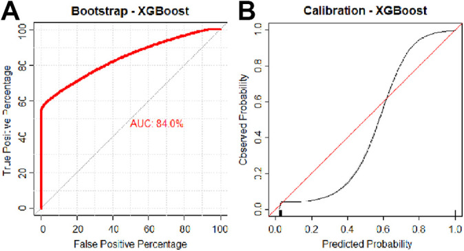
(A) Discrimination and (B) calibration of the extreme gradient boosted machine. AUC, area under the receiver operating characteristic curve.

The final model was calibrated with the observed frequencies within the test population and summarized in a calibration plot (Figure 1B). Ideally, the model is calibrated to a straight line, with an intercept of 0 and slope of 1 corresponding to perfect concordance of model predictions to observed frequencies in the data.

Model Implementation

The benefit of implementing the predictive algorithm into practice was assessed via decision curve analysis. These curves plot the net benefit against the predicted probabilities of each outcome, providing the cost-benefit ratio for every probability threshold of classifying a prediction as high risk. Additionally, curves demonstrating default strategies of changing management for all or no patients are included for comparative purposes.

Model Interpretability

Both global and local model interpretability and explanations were provided. Global model interpretability is provided as a plot of the model’s input variables normalized against the input considered to have the most contribution to the model prediction and Shapley Additive Explanations (SHAP), demonstrating how much each predictor contributes, either positively or negatively, to the model output. ²⁴ Local explanations are provided using local-interpretable model-agnostic explanations, in which variable contributions for individual model predictions are visually depicted. ^8,35

Digital Application

The final model was incorporated into a web-based application to illustrate possible future model integration. It should be noted that this digital application remains exclusively for research and educational purposes until rigorous external validation has been conducted. In the digital application, athlete demographic and performance data are entered to generate outcome predictions with accompanying explanations. All data analysis was performed in R Version 4.0.2 using RStudio Version 1.2.5001.

Results

Patient Characteristics

A total of 2103 NBA athletes were included in the study over a 20-year period. The median career length was 6 years (interquartile range, 2-9 years), with an almost even breakdown between designated positions (Table 1). Hamstring (36.4%) and calf (36.1%) injuries were more prevalent compared with quadriceps (11.5%) and groin (15.9%) injuries. The incidence rate of LEMSs per athlete per season was 5.83%.

Table 1.

Baseline Characteristic of the Study Population (N = 2103) ^a

Variable	Value
Age, y	26 (23-29)
BMI, kg/m2	24.3 (20.1-26.5)
Career length, y	6 (2-9)
Position
Center	384 (18.2)
Power forward	429 (20.4)
Point guard	424 (20.2)
Small forward	389 (18.5)
Shooting guard	477 (22.7)
Injuries (n = 736)
Quadriceps	85 (11.5)
Hamstring	268 (36.4)
Calf	266 (36.1)
Groin	117 (15.9)

^a Values are presented as n (%) or median (interquartile range). BMI, body mass index.

Multivariate Logistic Regression

After feature selection, the multivariate logistic regression was utilized to generate models using the selected features with odd ratios (ORs) of statistically significant contributors to LEMS. The most important risk factor for LEMS was previous injury count (OR, 21.0; 95% CI, 2.5-72.5) (Table 2). The next 5 most important risk factors for LEMS, in order from most to least contributory, were recent quadriceps injury (OR, 4.31; 95% CI, 1.21-15.4), recent groin injury (OR, 2.9; 95% CI, 2.88-2.91), free throw attempt rate (OR, 2.76; 95% CI, 1.27-6), recent ankle injury (OR, 2.66; 95% CI, 2.65-2.68), and recent hamstring injury (OR, 2.39; 95% CI, 2.38-2.4) (Table 2). While significant, age and games had a negligible effect in contributing to LEMS in the logistic regression (OR, 1.01-1.03), and 3-point attempt rate was protective of LEMS (OR, 0.46; 95% CI, 0.27-0.97).

Table 2.

Significant Contributors to Lower Extremity Muscle Strain From Logistic Regression Model ^a

Variable	OR (95% CI)
Previous injury count	21.0 (2.5-72.5)
Recent quadriceps injury	4.31 (1.21-15.4)
Recent groin injury	2.9 (2.88-2.91)
Free throw rate	2.76 (1.27-6)
Recent ankle injury	2.66 (2.65-2.68)
Recent hamstring injury	2.39 (2.38-2.4)
Recent concussion	2.34 (2.33-2.35)
Recent back injury	1.95 (1.94-1.96)
Age	1.03 (1.01-1.05)
Games played	1.01 (1.01-1.02)
3-point attempt rate	0.46 (0.27-0.79)

^a OR, odds ratio.

Model Creation and Performance

After multivariate logistic regression, machine-learning models were trained using the same variables identified from RFE. After model optimization, candidate model performances on internal validation were compared (Table 3). The random forest and XGBoost models had higher AUCs on internal validation data, 0.830 (95% CI, 0.829-0.831) and 0.840 (95% CI, 0.831-0.845), respectively, although XGBoost had a nonsignificantly higher Brier score. In this data set, conventional logistic regression had a significantly lower AUC on internal validation (0.818; 95% CI, 0.817-0.819) compared with the aforementioned models; similarly, this was lower than the AUC yielded by the simplified XGBoost model (0.832; 95% CI, 0.818-0.838). The calibration slope of models ranged from 0.997 for neural network to 1.003 for XGBoost, suggesting excellent estimation for all models (Table 3). The Brier score of models ranged from 0.029 for random forest to 0.31 for multiple models, indicating excellent accuracy. The XGBoost model had the highest overall AUC, with comparable calibration and Brier scores, and was therefore chosen as the best-performing candidate algorithm (Figure 1).

Table 3.

Model Assessment on Internal Validation Using 0.632 Bootstrapping With 1000 Resampled Data Sets (N = 2103) ^a

Metric	AUC (95% CI)
	Apparent	Internal Validation	Calibration Slope	Calibration Intercept	Brier Score
Elastic net	0.834 (0.791-0.877)	0.819 (0.818-0.820)	0.999 (0.998-1)	0.003 (0.001-0.005)	0.031 (0.027-0.034)
Random forest	0.905 (0.896-0.92)	0.830 (0.829-0.831)	1.001 (1-1.002)	0.002 (0.001-0.007)	0.029 (0.027-0.032)
XGBoost	0.906 (0.899-0.911)	0.840 (0.831-0.845)	1.003 (1.002-1.004)	0.002 (0.001-0.007)	0.03 (0.027-0.033)
SVM	0.881 (0.88-0.882)	0.787 (0.786-0.788)	0.999 (0.998-1)	0.007 (0.004-0.009)	0.031 (0.028-0.034)
Neural network	0.84 (0.839-0.841)	0.813 (0.812-0.814)	0.997 (0.996-0.998)	0.003 (0-0.005)	0.031 (0.028-0.034)
Logistic regression	0.835 (0.834-0.836)	0.818 (0.817-0.819)	0.998 (0.997-0.999)	0.008 (0.002-0.012)	0.031 (0.028-0.034)
Simple XGBoost	0.882 (0.880-0.882)	0.832 (0.818-0.838)	0.999 (0.998-1.000)	0.003 (0.002-0.004)	0.031 (0.027-0.033)

^a Null model Brier score = 0.063. AUC, area under the receiver operating characteristic curve; SVM, support vector machine; XGBoost, extreme gradient boosted.Data in parentheses is 95% confidence intervals.

Variable Importance

The global importance of input variables used for XGBoost was assessed with previous lower extremity injury having a near 100% relative influence, followed by games played, free throw attempt rate and percentage, 3-point attempt rate, and assist percentage (Figure 2A). SHAP values (Figure 2B) are average marginal contributions of selected features across all possible coalitions and indicate the 3 most common features to be total rebound percentage, previous lower extremity injury count, and games played. As can be interpreted, age and games played affect the model in a positive direction. While there are a number of outliers in which a high injury count does not contribute positively to an increased probability of LEMS, the overall contribution of previous injury count as indicated by the mean SHAP value remains positive.

Figure 2.

(A) Variable importance plot of the extreme gradient boosted (XGBoost) machine model. (B) Summary plot of Shapley (SHAP) values of the XGBoost model. Specifically, the global SHAP values are plotted on the x-axis with variable contributions on the y-axis. Numbers next to each input name indicate the mean global SHAP value, and gradient color indicates feature value. Each point represents a row in the original data set. Three-point attempt rate = percentage of player field goals that are for 3 points; free throw attempt rate = ratio of free throw attempts to field goal attempts. LE, lower extremity.

Decision Curve Analysis

Decision curve analysis was used to compare the net benefit derived from the trained XGBoost model. For comparison purposes, a decision curve was also plotted for a learned multivariate logistic regression model trained using the same parameters and inputs. The XGBoost model trained on the complete feature set demonstrated greater net benefit compared with logistic regression and other alternatives (Figure 3).

Figure 3.

Decision curve analysis comparing the complete extreme gradient boosted (XGBoost) machine algorithm with the complete logistic regression as well as a simplified model utilizing select parameters. The downsloping line marked by “All” plots the net benefit from the default strategy of changing management for all patients, while the horizontal line marked “none” represents the strategy of changing management for none of the patients (net benefit is zero at all thresholds). The “All” line slopes down because at a threshold of zero, false positives are given no weight relative to true positives; as the threshold increases, false positives gain increased weight relative to true positives and the net benefit for the default strategy of changing management for all patients decreases. LR, logistic regression.

Interpretation

An example of a patient-level evaluation and variable importance explanation is provided in Figure 4. This patient was assigned a probability of 0.007 (approximately 1%) for sustaining LEMS. Features that decreased the patient’s risk for LEMS included lack of recent ankle injury; concussion; or groin, hamstring, quadriceps, or back injury (among others). Features that increased the patient’s risk of injury were a recent back injury in addition to 3-point shot percentage.

Figure 4.

Example of individual patient-level explanation for the simplified extreme gradient boosted machine algorithm predictions. This athlete had a predicted injury risk of 0.77% at this point during the season. The only feature to support the likelihood of injury was a recent back injury.

For each patient or professional basketball athlete, baseline parameters can be collected or examined during the encounter to generate predictions regarding risk of LEMS in the athlete. These predictions can be utilized to inform counseling, modify exercise regiments, or dictate rest periods for athletes at high risk for LEMS. The final model was incorporated into a web-based application that generated predictions for probabilities of LEMS. The application (available at https://sportsmed.shinyapps.io/NBA_LE) is accessible from desktop computers, tablet computers, and smartphones. Default values are provided as placeholders in the interface, and the model requires complete cases to generate predictions and explanations.

Discussion

The principal findings of our study are that (1) the incidence of LEMSs in the NBA over the study period was 5.83%, and a number of significant features in the prediction of these injuries were identified; (2) the XGBoost algorithms outperformed logistic regression with regard to discrimination, calibration, and overall performance; and (3) the clinical model was incorporated into an open-access injury risk calculator for education and demonstration purposes.

Despite a number of studies evaluating injuries in the NBA, ^20,36,37 there is a paucity of evidence regarding the rate of LEMS. A study by Drakos et al ⁶ found that hamstring strains (n = 413; 3.3%), defined as any that required missed time, physician referral, or emergency care, were among the most frequently encountered orthopaedic injuries in the NBA across a 17-year study period; our study reports a lower incidence (n = 268) over 20 years, likely given our accounting of only time-loss injuries. This likely reflects a similar overall deflation of injury incidence in our cohort among other body parts.

While similar investigations have been carried out in professional soccer, baseball, and American football athletes, ^21,28,32 few studies have previously investigated the risk factors for characterizing the epidemiology of LEMSs in professional basketball athletes. The input features that were significant on both multivariate logistic regression and global variable importance assessment included the following: previous injury count; games played; history of recent ankle, groin, hamstring, or back injury; history of a concussion; free throw percentage; and 3-point shot percentage. The investigation by Orchard et al ³² identified a strong relationship between LEMS and a recent history of same-site muscle strain. We similarly utilized the definition of recent recurrence as within 8 weeks of the index injury as described by Fuller et al, ⁷ because of the absence of such a consensus definition in the NBA, and corroborated this finding among basketball athletes. This relationship is intuitive, as premature return to play can predispose athletes to reinjury. However, we did not identify a relationship between nonrecent history of any injuries with the risk of an index injury, which suggests that injury risk for LEMSs may be equivalent between controls and injured athletes beyond the 8-week window within this cohort of elite athletes.

There has been a longstanding relationship between ankle injuries and lower extremity biomechanics and postural stability. ^2,22,23 However, whether this relationship is causative or correlative is more ambiguous. While a motion analysis study by Leanderson et al ²² identified a significantly increased range of postural sway among Swedish Division II basketball players with a history of lateral ankle sprains compared with controls, a more recent investigation by Lopezosa-Reca et al ²³ found that athletes who had certain foot postures as described by the Foot Posture Index were more likely to experience lower extremity injuries such as lateral ankle sprains and patellar tendinopathy. Our findings suggest that altered foot biomechanics secondary to a recent ankle injury contribute at least partially to the increased risk of lower extremity muscle injuries, as nonrecent ankle injury was not found to be a significant risk factor.

The relationship between concussion and lower extremity injury has been extensively studied in the sports medicine literature, ^10,15,16 with a number of hypotheses for the underlying mechanism, including resultant deficiencies in dynamic balance, neuromuscular control, cognitive accuracy, and gait performance. ^{4,14,27,31,40} This observation is corroborated by our study, which identified a concussion history as a significant risk factor in both the multivariate logistic regression and the machine learning models. Finally, an interesting protective correlation was identified between 3-point attempt rate and risk of lower extremity injury. One possible reason for this observation may lie in the role of the 3-point attempt rate as a proxy of playing style, as players who take a greater number of 3-point attempts usually play a less physical perimeter game. Conversely, the free throw rate represents the ability of a player to draw personal fouls from opponents and therefore is a measure of physical play and a strong predictor of injury risk.

On evaluation of the predictive models, both the complete and simple XGBoost models outperformed the logistic regression on both discrimination and the Brier score. Investigators have previously developed machine learning injury-prediction models for recreational athletes ¹⁷ as well as in professional sports, including the NFL, ⁴² National Hockey League, ²⁶ and MLB. ¹⁸ These models utilized a range of inputs, from performance metrics to video recordings and motion kinematics. The present study evaluated a number of performance metrics as well as clinical injury history, which may present more actionable findings for the team physician. After external validation, prospective deployment of the model can integrate the athlete’s injury history in an 8-week window to provide a real-time snapshot of the athlete’s risk for experiencing a LEMS with excellent fidelity and reliability. Additionally, with contemporary improvements in computational and sensor technology, there has also been an increase in focus on the potential of global positioning system tracking data in real-time injury forecasting and prevention, ⁹ and machine learning technology is uniquely equipped to handle the sheer overabundance of data available through the automation of structure and pattern recognition. ¹²

Strengths and Limitations

The strengths of this study must be interpreted concurrently with a number of limitations. The first concerns the quality of the data source. While we were able to capture injury history and performance metrics that can serve as proxies for playing style, data extracted from publicly available sources do not offer insight into postinjury rehabilitation protocol or long-term management strategies for recurrent injuries. Additionally, detailed clinical data including physical examination and imaging findings were unavailable. Within these limitations, it is notable that the current machine learning algorithm reached an excellent level of concordance and calibration and that a simplified algorithm performed similarly to the complete logistic regression model; it should be within expectation that prospective incorporation of granular characteristics of the injury and the return-to-play protocol can continue to augment the performance of the algorithm. Second, the sampling remains limited to the population of elite athletes, and generalizability to those competing at the recreational or semiprofessional levels may remain questionable until further external validation, as such use of the digital application is for education and demonstration only. In this context, an interesting future extension of this study may be a matched-cohort comparison of LEMS injury risk between professional and amateur athletes. Finally, the black box phenomenon is an inherent flaw of certain machine learning algorithms wherein transparency into model behavior is insufficient. For example, the complete model utilizes 25 inputs and can become extremely cumbersome for the user, especially for physicians to whom the effects of specific performance variables may not be clear from a clinical perspective. We have attempted to mitigate this by reducing the dimensions of the training data to produce a simplified model that is both clinically sound and easily deployable without significantly sacrificing its effectiveness. In addition, the application features a built-in local agnostic model explanation algorithm that can approximate the model dependence on each input for a given prediction.

Conclusion

Machine-learning algorithms such as XGBoost outperformed logistic regression in the effective and reliable prediction of a LEMS that will result in lost time. Factors resulting in an increased risk of LEMS included history of a back, quadriceps, hamstring, groin, or ankle injury; concussion within the previous 8 weeks; and total count of previous injuries.

APPENDIX

DETAILED MACHINE-LEARNING MODELING WORKFLOW

Missing Data

Features with missing data were imputed utilizing the MissForest multiple imputation method to reduce bias and improve statistical robustness. ⁴ If a variable was considered important and missing in more than 30% of the study population, complete case analysis was performed after exclusion of incomplete cases. The MissForest multiple imputation method was used to impute remaining variables with less than 30% missing data ^5,13,14 ; variables were assumed to be missing at random based on epidemiological convention. ^8,10

Modeling

After imputation for missing data, highly collinear variables (defined as Spearman correlation coefficients >0.5 or those considered clinically confounding) were identified and excluded. Notably, we did not explicitly exclude outcome variables of one model as input features in other models; therefore, recurrence was considered an input feature in the model for progression to surgery, and whether patients underwent surgical treatment was considered an input feature in the model for the development of symptomatic osteoarthritis.

The following 5 algorithms were developed on the training data set: (1) support vector machines, (2) elastic net penalized logistic regression, (3) random forest, (4) multilayer perceptron, and (5) XGBoost. These algorithms have been shown to develop robust predictive models for various orthopaedic conditions. ⁶ Each model was trained and validated via 0.632 bootstrapping with 1000 resampled data sets, also known as Monte Carlo cross-validation. In brief, model evaluation consists of reiterative partitions of the complete data set into train and test sets. For each combination of train and test set, the model is trained on the train set using 10-fold cross-validation repeated 3 times. ¹¹ The performance of this model is then evaluated on the respective test set, and no data points from the training set were included in the test set. This sequence of steps is then repeated for 999 more data partitions. The model is thus trained and tested on all data points available, and evaluation metrics are summarized with standard distributions of values. Bootstrapping has been found to optimize both model bias and variance and improve overall performance compared with internal validation through splitting the data into a partition of training and holdout sets. ¹⁵ In addition, a gradient boosted ensemble model of the 5 candidate models was constructed and trained, similarly through 0.623 bootstrapping. The advantages of ensemble modeling include decreasing variance and bias as well as improving predictions, while disadvantages include increased memory requirements and reduced speed of implementation. ¹

Model Assessment

Model performance for each algorithm was assessed for (1) discrimination by comparing area under the receiver operating characteristic curve, with >0.80 defined as excellent concordance based on the works of Hosmer and Lemeshow ³ ; (2) calibration by calibration curve plots, intercept, and slope; (3) decision curve analysis; and (4) Brier score, which is the mean square difference between predicted probabilities of models and observed outcomes. The Brier score for each algorithm was compared with the null Brier score, which is calculated by assigning each patient a probability equivalent to the population prevalence of the predicted outcome.

Decision curve analysis was used to compare the benefit of implementing the best-performing algorithm to the logistic regression in practice. ¹⁶ The curve plots net benefit against the predicted probabilities of each outcome and provides the cost-benefit ratio for every value of the predicted probability. These ratios provide useful guidance for individualized decision making and account for variability in clinician and patient thresholds for what is considered high risk. Additionally, decision curves for the default strategies of changing management for no patients or all patients are plotted for comparison purposes. Equations for the calculation of the cost-benefit ratio and net benefit are as follows:

$$Costbenefitratio=\frac{Riskthresholdprobability}{1-Riskthresholdprobability}$$

$$Netbenefit=\frac{Truepositives-Costbenefitratio\left(falsepositives\right)}{Totalnumberofpatients}$$

Both global and local model interpretability and explanations were provided. The global model variable importance plot demonstrates variable importance normalized to the input considered most contributory to the model predictive power. Local explanations for model behavior were provided for transparency into each individual output using local-interpretable model-agnostic explanations. ^2,12 The explanation algorithm generates optimized fits based on an established distance measure for the predicted probabilities of each outcome label based on the values of both categorical and continuous input, which can be plotted for visualization. ^2,12

Appendix Table A1.

Definition of Machine Learning Concepts and Methods Used

Term	Definition
Multiple imputation	A popular method for handling missing data, which are often a source of bias and error in model output. In this approach, a missing value in the data set is replaced with an imputed value based on a statistical estimation; this process is repeated randomly, resulting in multiple “completed” data sets, each consisting of observed and imputed values. These are combined utilizing a simple formula known as the Rubin rule to give final estimates of target variables. 9
Recursive feature elimination (RFE)	A feature selection algorithm that searches for an optimal subset of features by fitting a given machine learning algorithm (random forest and naïve Bayes in our case) to the predicted outcome, ranking the features by importance, and removing the least important features; this is done repeatedly, in a “recursive” manner, until a specified number of features remains or a threshold value of a designated performance metric has been reached. The features can then be entered as inputs into the candidate models for prediction of the desired outcome. 7
0.632 bootstrapping	The method for training an algorithm based on the input features selected from RFE. Briefly, model evaluation consists of reiterative partitions of the complete data set into train and test sets. For each combination of train and test set, the model is trained on the train set using 10-fold cross-validation repeated 3 times. The performance of this model is then evaluated on the respective test set, and no data points from the training set were included in the test set. This sequence of steps is then repeated for 999 more data partitions. 11 The model is thus trained and tested on all data points available, and evaluation metrics are summarized with standard distributions of values. 11 Bootstrapping has been found to optimize both model bias and variance and improve overall performance compared with internal validation through splitting of the data into training and holdout sets.
Extreme gradient boosting	Algorithm of choice among stochastic gradient boosting machines, a family in which multiple weak classifiers (a classifier that predicts marginally better than random) are combined (in a process known as boosting) to produce an ensemble classifier with a superior generalized misclassification error rate. 7
Random forest	Algorithm of choice among tree-based algorithms, an ensemble of independent trees, each generating predictions for a new sample chosen from the training data, and whose predictions are averaged to give the forest’s prediction. The ensembling process is distinct in principle from gradient boosting. 7
Neural network	A nonlinear regression technique based on 1 or more hidden layers consisting of linear combinations of some or all predictor variables, through which the outcome is modeled; these hidden layers are not estimated in a hierarchical fashion. The structure of the network mimics neurons in a brain. 7
Elastic net penalized logistic regression	A penalized linear regression based on a function to minimize the square errors of the outputs; belongs to the family of penalized linear models, including ridge regression and the lasso. 7
Support vector machines	A supervised learning algorithm that performs classification problems by representing each data point as a point in abstract space and defining a plane known as a hyperplane that separates the points into distinct binary classes, with maximal margin. Hyperplanes can be linear or nonlinear, as we have implemented in the presented analysis, using a circular kernel. 7
Area under the receiver operating characteristic curve (AUC)	A common metric to model performance, utilizing the receiver operating characteristic curve, which plots calculated sensitivity and specificity given the class probability of an event occurring (instead of using a 50:50 probability). The AUC classically ranges from 0.5 to 1, with 0.5 being a model that is no better than random and 1 being a model that is completely accurate in assigning class labels. 7
Calibration	The ability of a model to output probability estimates that reflect the true event rate in repeat sampling from the population. An ideal model is a straight line with an intercept of 0 and slope of 1 (ie, perfect concordance of model predictions to observed frequencies within the data). A model can correctly assign a label, as reflected by the AUC, yet it can output class probabilities of a binary outcome that is dramatically different from its true event rate in the population; such a model is not well calibrated. 7
Brier score	The mean square difference between predicted probabilities of models and observed outcomes in the testing data. The Brier score can generally range from 0 for a perfect model to 0.25 for a noninformative model. 7
Decision curve analysis	A measure of clinical utility whereby a clinical net benefit for 1 or more prediction models or diagnostic tests is calculated in comparison with default strategies of treating all or no patients. This value is calculated based on a set threshold, defined as the minimum probability of disease at which further intervention would be warranted. The decision curve is constructed by plotting the ranges of threshold values against the net benefit yielded by the model at each value; as such, a model curve that is farther from the bottom left corner yields more net benefit than one that is closer. 16

Appendix Table A2.

Inputs Considered for Feature Selection

Variables

Recent groin injury Recent ankle injury Recent concussion Recent hamstring injury Recent back injury Age Recent quad injury Previous injury count Position Games played Games started Minutes per game Field goals made per game Field goal attempts per game Field goal percentage 3-point shots made per game 3-point shots attempted per game 3-point percentage 2-point shots made per game 2-point shots attempted per game 2-point percentage Effective field goal percentage Free throws made per game Free throws attempted per game Free throw percentage Offensive rebounds per game Defensive rebounds per game Total rebounds per game Assists per game Steals per game Blocks per game Turnovers per game Personal fouls per game Points per game Player efficiency rating True shooting percentage 3-point attempt rate Free throw attempt rate Offensive rebound percentage Defensive rebound percentage Total rebound percentage Assist percentage Steals percentage Blocks percentage Turnover percentage Usage percentage Offensive win share Defensive win share Win shares Win shares per 48 min Offensive box ± Defensive box ± Box ± Value over replacement player

References

- 1. Camp CL, Dines JS, van der List JP, et al. Summative report on time out of play for Major and Minor League Baseball: an analysis of 49,955 injuries from 2011 through 2016. Am J Sports Med. 2018;46(7):1727–1732. [DOI] [PubMed] [Google Scholar]
- 2. Cheng WL, Jaafar Z. Effects of lateral ankle sprain on range of motion, strength and postural balance in competitive basketball players: a cross-sectional study. J Sports Med Phys Fitness. 2020;60(6):895–902. [DOI] [PubMed] [Google Scholar]
- 3. Collins GS, Reitsma JB, Altman DG, Moons KG. Transparent reporting of a multivariable prediction model for individual prognosis or diagnosis (TRIPOD): the TRIPOD statement. Br J Surg. 2015;102(3):148–158. [DOI] [PubMed] [Google Scholar]
- 4. Cripps A, Livingston S, Jiang Y, et al. Visual perturbation impacts upright postural stability in athletes with an acute concussion. Brain Inj. 2018;32(12):1566–1575. [DOI] [PubMed] [Google Scholar]
- 5. Darst BF, Malecki KC, Engelman CD. Using recursive feature elimination in random forest to account for correlated variables in high dimensional data. BMC Genet. 2018;19(suppl 1):65. [DOI] [PMC free article] [PubMed] [Google Scholar]
- 6. Drakos MC, Domb B, Starkey C, Callahan L, Allen AA. Injury in the National Basketball Association: a 17-year overview. Sports Health. 2010;2(4):284–290. [DOI] [PMC free article] [PubMed] [Google Scholar]
- 7. Fuller CW, Ekstrand J, Junge A, et al. Consensus statement on injury definitions and data collection procedures in studies of football (soccer) injuries. Br J Sports Med. 2006;40(3):193–201. [DOI] [PMC free article] [PubMed] [Google Scholar]
- 8. Greenwell BM, Boehmke BC, McCarthy AJ. A simple and effective model-based variable importance measure. arXiv. Preprint posted online May 12, 2018. doi:10.48550/arXiv.1805.04755 [Google Scholar]
- 9. Guitart M, Casals M, Casamichana D, et al. Use of GPS to measure external load and estimate the incidence of muscle injuries in men’s football: a novel descriptive study. PLoS One. 2022;17(2):e0263494. [DOI] [PMC free article] [PubMed] [Google Scholar]
- 10. Harada GK, Rugg CM, Arshi A, Vail J, Hame SL. Multiple concussions increase odds and rate of lower extremity injury in National Collegiate Athletic Association athletes after return to play. Am J Sports Med. 2019;47(13):3256–3262. [DOI] [PubMed] [Google Scholar]
- 11. Harrell FE, Jr. Regression Modeling Strategies: With Applications to Linear Models, Logistic and Ordinal Regression, and Survival Analysis. Springer; 2015. [Google Scholar]
- 12. Helm JM, Swiergosz AM, Haeberle HS, et al. Machine learning and artificial intelligence: definitions, applications, and future directions. Curr Rev Musculoskelet Med. 2020;13(1):69–76. [DOI] [PMC free article] [PubMed] [Google Scholar]
- 13. Hosmer DW, Lemeshow S, Sturdivant RX. Applied Logistic Regression. 3rd ed. Wiley ; 2013. [Google Scholar]
- 14. Howell DR, Lynall RC, Buckley TA, Herman DC. Neuromuscular control deficits and the risk of subsequent injury after a concussion: a scoping review. Sports Med. 2018;48(5):1097–1115. [DOI] [PMC free article] [PubMed] [Google Scholar]
- 15. Hunzinger KJ, Costantini KM, Swanik CB, Buckley TA. Diagnosed concussion is associated with increased risk for lower extremity injury in community rugby players. J Sci Med Sport. 2021;24(4):368–372. [DOI] [PubMed] [Google Scholar]
- 16. Hunzinger KJ, Radzak KN, Costantini KM, Swanik CB, Buckley TA. Concussion history is associated with increased lower-extremity injury incidence in Reserve Officers’ Training Corps cadets. BMJ Mil Health. Published online October 29, 2020. doi:10.1136/bmjmilitary-2020-001589 [DOI] [PubMed] [Google Scholar]
- 17. Jauhiainen S, Kauppi JP, Leppänen M, et al. New machine learning approach for detection of injury risk factors in young team sport athletes. Int J Sports Med. 2021;42(2):175–182. [DOI] [PubMed] [Google Scholar]
- 18. Karnuta JM, Luu BC, Haeberle HS, et al. Machine learning outperforms regression analysis to predict next-season Major League Baseball player injuries: epidemiology and validation of 13,982 player-years from performance and injury profile trends, 2000-2017. Orthop J Sports Med. 2020;8(11):2325967120963046. [DOI] [PMC free article] [PubMed] [Google Scholar]
- 19. Karnuta JM, Navarro SM, Haeberle HS, et al. Predicting inpatient payments prior to lower extremity arthroplasty using deep learning: which model architecture is best? J Arthroplasty. 2019;34(10):2235–2241.e2231. [DOI] [PubMed] [Google Scholar]
- 20. Khan M, Madden K, Burrus MT, et al. Epidemiology and impact on performance of lower extremity stress injuries in professional basketball players. Sports Health. 2018;10(2):169–174. [DOI] [PMC free article] [PubMed] [Google Scholar]
- 21. Kokubu T, Mifune Y, Kanzaki N, et al. Muscle strains in the lower extremity of Japanese professional baseball players. Orthop J Sports Med. 2020;8(10):2325967120956569. [DOI] [PMC free article] [PubMed] [Google Scholar]
- 22. Leanderson J, Wykman A, Eriksson E. Ankle sprain and postural sway in basketball players. Knee Surg Sports Traumatol Arthrosc. 1993;1(3-4):203–205. [DOI] [PubMed] [Google Scholar]
- 23. Lopezosa-Reca E, Gijon-Nogueron G, Morales-Asencio JM, Cervera-Marin JA, Luque-Suarez A. Is there any association between foot posture and lower limb-related injuries in professional male basketball players? A cross-sectional study. Clin J Sport Med. 2020;30(1):46–51. [DOI] [PubMed] [Google Scholar]
- 24. Lundberg SM, Lee S. A unified approach to interpreting model predictions. Adv Neural Inf Process Syst. 2017:4765–4774. [Google Scholar]
- 25. Luo W, Phung D, Tran T, et al. Guidelines for developing and reporting machine learning predictive models in biomedical research: a multidisciplinary view. J Med Internet Res. 2016;18(12):e323. [DOI] [PMC free article] [PubMed] [Google Scholar]
- 26. Luu BC, Wright AL, Haeberle HS, et al. Machine learning outperforms logistic regression analysis to predict next-season NHL player injury: an analysis of 2322 players from 2007 to 2017. Orthop J Sports Med. 2020;8(9):2325967120953404. [DOI] [PMC free article] [PubMed] [Google Scholar]
- 27. Lynall RC, Blackburn JT, Guskiewicz KM, et al. Reaction time and joint kinematics during functional movement in recently concussed individuals. Arch Phys Med Rehabil. 2018;99(5):880–886. [DOI] [PubMed] [Google Scholar]
- 28. Mack CD, Kent RW, Coughlin MJ, et al. Incidence of lower extremity injury in the National Football League: 2015 to 2018. Am J Sports Med. 2020;48(9):2287–2294. [DOI] [PubMed] [Google Scholar]
- 29. Navarro SM, Wang EY, Haeberle HS, et al. Machine learning and primary total knee arthroplasty: patient forecasting for a patient-specific payment model. J Arthroplasty. 2018;33(12):3617–3623. [DOI] [PubMed] [Google Scholar]
- 30. Nwachukwu BU, Beck EC, Lee EK, et al. Application of machine learning for predicting clinically meaningful outcome after arthroscopic femoroacetabular impingement surgery. Am J Sports Med. 2020;48(2):415–423. [DOI] [PubMed] [Google Scholar]
- 31. Oldham JR, Howell DR, Knight CA, Crenshaw JR, Buckley TA. Gait performance is associated with subsequent lower extremity injury following concussion. Med Sci Sports Exerc. 2020;52(11):2279–2285. [DOI] [PMC free article] [PubMed] [Google Scholar]
- 32. Orchard JW, Chaker Jomaa M, Orchard JJ, et al. Fifteen-week window for recurrent muscle strains in football: a prospective cohort of 3600 muscle strains over 23 years in professional Australian rules football. Br J Sports Med. 2020;54(18):1103–1107. [DOI] [PubMed] [Google Scholar]
- 33. Powell JW, Dompier TP. Analysis of injury rates and treatment patterns for time-loss and non-time-loss injuries among collegiate student-athletes. J Athl Train. 2004;39(1):56–70. [PMC free article] [PubMed] [Google Scholar]
- 34. Ramkumar PN, Navarro SM, Haeberle HS, et al. Development and validation of a machine learning algorithm after primary total hip arthroplasty: applications to length of stay and payment models. J Arthroplasty. 2019;34(4):632–637. [DOI] [PubMed] [Google Scholar]
- 35. Ribeiro MT, Singh S, Guestrin C. Model-agnostic interpretability of machine learning. arXiv. Preprint posted online June 16, 2016. doi:10.48550/arXiv.1606.05386 [Google Scholar]
- 36. Schallmo MS, Fitzpatrick TH, Yancey HB, et al. Return-to-play and performance outcomes of professional athletes in North America after hip arthroscopy from 1999 to 2016. Am J Sports Med. 2018;46(8):1959–1969. [DOI] [PubMed] [Google Scholar]
- 37. Starkey C. Injuries and illnesses in the National Basketball Association: a 10-year perspective. J Athl Train. 2000;35(2):161–167. [PMC free article] [PubMed] [Google Scholar]
- 38. Steyerberg EW, Harrell FE, Jr. Prediction models need appropriate internal, internal-external, and external validation. J Clin Epidemiol. 2016;69:245–247. [DOI] [PMC free article] [PubMed] [Google Scholar]
- 39. Steyerberg EW, Moons KG, van der Windt DA, et al. Prognosis Research Strategy (PROGRESS) 3: prognostic model research. PLoS Med. 2013;10(2):e1001381. [DOI] [PMC free article] [PubMed] [Google Scholar]
- 40. Walker WC, Nowak KJ, Kenney K, et al. Is balance performance reduced after mild traumatic brain injury? Interim analysis from Chronic Effects of Neurotrauma Consortium (CENC) multi-centre study. Brain injury. 2018;32(10):1156–1168. [DOI] [PubMed] [Google Scholar]
- 41. Werner BC, Belkin NS, Kennelly S, et al. Acute gastrocnemius-soleus complex injuries in National Football League athletes. Orthop J Sports Med. 2017;5(1):2325967116680344. [DOI] [PMC free article] [PubMed] [Google Scholar]
- 42. Wu LC, Kuo C, Loza J, et al. Detection of American football head impacts using biomechanical features and support vector machine classification. Sci Rep. 2017;8(1):855. [DOI] [PMC free article] [PubMed] [Google Scholar]