Automated Adult Epilepsy Diagnostic Tool Based on Interictal Scalp Electroencephalogram Characteristics: A Six-Center Study

Abstract

The diagnosis of epilepsy often relies on a reading of routine scalp electroencephalograms (EEGs). Since seizures are highly unlikely to be detected in a routine scalp EEG, the primary diagnosis depends heavily on the visual evaluation of Interictal Epileptiform Discharges (IEDs). This process is tedious, expert-centered, and delays the treatment plan. Consequently, the development of an automated, fast, and reliable epileptic EEG diagnostic system is essential. In this study, we propose a system to classify EEG as epileptic or normal based on multiple modalities extracted from the interictal EEG. The ensemble system consists of three components: a Convolutional Neural Network (CNN)-based IED detector, a Template Matching (TM)-based IED detector, and a spectral feature-based classifier. We evaluate the system on datasets from six centers from the USA, Singapore, and India. The system yields a mean Leave-One-Institution-Out (LOIO) cross-validation (CV) area under curve (AUC) of 0.826 (balanced accuracy (BAC) of 76.1%) and Leave-One-Subject-Out (LOSO) CV AUC of 0.812 (BAC of 74.8%). The LOIO results are found to be similar to the interrater agreement (IRA) reported in the literature for epileptic EEG classification. Moreover, as the proposed system can process routine EEGs in a few seconds, it may aid the clinicians in diagnosing epilepsy efficiently.

1. Introduction

Epilepsy is a group of chronic brain disorders that are characterized by unprovoked recurrent seizures. According to recent statistics, it affects about 70 million people in the world.¹ The routine scalp electroencephalogram (EEG) is widely utilized as a fundamental medical test for the diagnosis of epilepsy.² Seizures or ictal events are highly unlikely to occur during a routine scalp EEG recording. Interictal Epileptiform Discharges (IEDs), on the other hand, are traditional biomarkers of epilepsy.³ An automated IED detection system is highly beneficial for the clinical assessment and treatment of epilepsy. This system could be applied predominantly for three purposes: epilepsy diagnosis, analyzing the effect of antiepileptic medications and assessing the risk of seizure reoccurrence, and for pre-surgical planning (localization of epileptic foci).^4,5 In this paper, we consider the use case of diagnosing epilepsy. For the purpose of diagnosing epilepsy, neurologists are less concerned about the exact number IEDs in the EEG, but rather whether any IEDs are present. Consequently, EEG-level classification (whether it is epileptic or normal) is the main objective, instead of detecting individual IEDs.

In the literature, studies have been performed to identify abnormal EEGs. Roy et al. have presented the ChronoNet⁶ which achieves an accuracy of 86.6% on the Temple University Hospital (TUH) Abnormal Corpus.^7,8 Gemein et al. have consolidated different studies on the same database and have given a review of the literature on abnormal EEG classification.⁹ However, there are only limited studies that consider the problem of classifying epileptic EEGs (EEGs that exhibit interictal/ictal epileptiform patterns) versus normal EEGs (EEGs that do not exhibit any abnormality). Schmidt et al. have proposed a new computational biomarker for classifying EEGs of patients with idiopathic generalized epilepsy (IGE) with normal EEGs.¹⁰ They achieved a maximum balanced accuracy (BAC) of 82.9% for classifying 30 epileptic EEGs and 38 nonepileptic EEGs. However, the evaluation was performed on 20-s artifact-free segments that were visually selected by an expert.¹⁰

In our preliminary study from 2018, we proposed a Support Vector Machine (SVM)¹¹-based epileptic EEG classifier with IED detection features derived from a one-dimensional (1D) Convolutional Neural Network (CNN), on a small dataset of 154 EEGs.¹² We achieved a mean four-fold EEG classification area under curve (AUC) of 0.87 with an accuracy of 83.86%. In a parallel work to this study, Jing et al. proposed a two-dimensional (2D) CNN output-based EEG classifier that achieved an AUC of 0.847 to classify EEGs with and without IEDs.¹³ These two studies^12,13 were performed exclusively on datasets from a single center, and consider only a single method for EEG classification. We exclude the literature^14,15 based on the Bonn EEG dataset¹⁶ and Bern–Barcelona dataset,¹⁷ since these datasets only contain single-channel EEG segments without any clinical information such as patient details, channel location, etc. Most studies on those two datasets that claim to have achieved “epileptic EEG classification” have only been tested on hand-picked segments of EEG rather than the whole EEG. Therefore, these studies do not represent real-world clinical scenarios.

To address those shortcomings, we combine multiple approaches to classify EEGs, and assess those methods on EEG data from multiple centers. Specifically, we explore two types of IED detectors, based on CNN and template matching (TM), respectively, in addition to a classifier that leverage spectral information. We follow the methodology proposed in our previous work to design the CNN¹⁸ and TM IED detector.^19,20 CNN IED detectors have shown superior performance than traditional IED detectors as well as noninferiror performance to experts.^13,18 For the TM IED detector, the IED library is developed by applying affinity propagation (AP)²¹ in conjunction with Dynamic Time Warping (DTW).²² We apply correlation coefficient²³ as distance measure for the TM IED detector.¹⁹ Since correlation is invariant to scaling, the TM IED detector is invariant to EEG amplitude scaling. In addition, spectral features have been shown to discriminate epileptic and normal EEGs.²⁴ For the spectral feature-based classifier, we compute relative power features in the five standard EEG frequency bands (delta, theta, alpha, beta, and gamma), and with those relative power values as features, we apply an SVM with Gaussian kernel,¹¹ since it has been shown to perform well in the literature.²⁵ The TM and EEG spectral feature-based detectors are more explainable, easier to understand, and invariant to amplitude scaling. On the other hand, the CNN IED detector offers fewer misclassifications for detecting IEDs.

We evaluate the proposed systems on EEG data from six centers. We employ the dataset from Massachusetts General Hospital (MGH)¹⁸ as the primary dataset to train and validate the IED detectors. The evaluation of the other datasets is performed considering two real-world scenarios. In the first scenario, we wish to apply our proposed system to EEG data of a center that is not included in the current study, and assume that we have access to a small dataset of EEGs and corresponding reports from this center. Here, we would be able to calibrate the EEG classification system on dataset from the new center. To assess our system in this scenario, we compute Leave-One-Subject-Out (LOSO) cross-validation (CV) for each individual center. In the second scenario, we assume that we do not have any prior information regarding the EEGs from the center. This scenario is evaluated by Leave-One-Institution-Out (LOIO) CV. As far as we know, the current study might be the first to perform a cross-institutional assessment of epileptic EEG classification. It is indeed necessary to perform LOIO CV to establish the clinical validity of a diagnostic tool. The proposed system achieves an LOIO CV mean AUC of 0.826 (mean BAC of 76.1%) that corroborated with the interrater agreement (IRA) reported in the literature for discriminating epileptic EEGs from normal EEGs.

The rest of this paper is organized as follows. We describe the EEG datasets and preprocessing steps in Sec. 2.1, and the methodology applied to design and evaluate the proposed system in Secs. 2.2 and 2.3, respectively. In Sec. 3, we present the results, while in Sec. 4, we provide a discussion, and elaborate on the limitations of this study. In Sec. 5, we offer concluding remarks, and suggest several topics for future research.

2. Materials and Methods

2.1. Scalp EEG dataset

We analyzed routine scalp EEG recordings from six centers across the globe:

1. MGH, Boston, USA.

2. TUH, USA (public dataset⁸).

3. National University Hospital (NUH), Singapore.

4. National Neuroscience Institute (NNI), Singapore.

5. Fortis Hospital Mulund, Mumbai, India.

6. Lokmanya Tilak Municipal General Hospital (LTMGH), Mumbai, India.

The scalp EEGs were recorded according to the International 10–20 electrode system at different sampling frequencies. We categorize the EEGs into two types according to the clinical report: epileptic EEGs (containing IEDs or seizures), and normal EEGs, which do not exhibit any abnormalities. Along with the overall EEG assessment (epileptic or normal), we also extract the following additional information: the presence of ictal events in the EEG and the patient’s history of seizures. Details about the different datasets are presented in Table 1.

Table 1.

Information about the six datasets investigated in this study.

Dataset/Fs	Number of epileptic EEGs/Duration (minutes)	Number of patients	Gender (Age in years)	Number of non-epileptic EEGs/Duration (minutes)	Number of non-epileptic patients	Gender (Age in years)
MGH 128 Hz, 200 Hz, 256 Hz	93 26.4±4.5	84	M 43 (35.2±27.2) F 41 (37.1±28.2)	461 31.2±9.8	461	Adult EEGs Gender UNK
NUH 250 Hz	96 19.6±10.1	96	M 54 (54.6±20.9) F 42 (59.7±20.0)	99 18.3±7.4	99	M 60 (48.8±17.9) F 39 (50.8±20.4)
NNI 200 Hz	121 26.8±2.2	121	M 56 (44.8±19.0) F 65 (46.9±21.0)	118 26.6±1.3	118	M 60 (44.1±16.7) F 58 (51.2±18.4)
TUH 250 Hz, 256 Hz, 500 Hz	485 12.3±7.0	47	M 16 (47.6±16.5) F 31 (56.5±16.4)	44+163 15.8±8.5	30+33	M 26 (52.1±14.7) F 36 (47.4±16.7 UNK for 1 EEG
Fortis 500 Hz	36 22.8±6.8	36	M 25 (37.0±14.7) F 10 (38.4±17.4) UNK gender for 1 EEG (25)	343 20.5±5.3	343	M 185 (48.5±18.1) F 147 (47.2±17.3) UNK gender for 11 EEGs (41.0±18.5)
LTMGH 256 Hz	44 14.6±2.1	44	M 26 (51.2±24.3) F 18 (46.4±24.6)	626 13.8±1.4	626	M 365 (41.0±16.7) F 261 (41.4±19.0)
Total	875 250.1 hours	427	-	1854 637.9 hours	1710	-

Notes: All the EEGs are recorded from 19 channels. F_s: sampling frequency; M: male; F: female. UNK: unknown; “+”: multiple sets, duration/age are reported as mean ± standard deviation.

The MGH dataset consists of 18,164 IEDs (from 93 epileptic EEGs) annotated by two neurologists. The annotations were performed with the aid of NeuroBrowser (NB) software.²⁶ The NUH and NNI datasets consist of routine scalp EEGs recorded during the routine clinical care at NUH and NNI Singapore, respectively. The TUH database⁸ is the largest public epileptic EEG database. In our analysis, we consider the TUH Epilepsy corpus²⁷ that contains routine scalp EEGs, recorded sometimes over multiple sessions, from 133 patients with epilepsy (1360 EEGs) and 104 patients without epilepsy (288 EEGs). We select the EEGs with a duration range of 5–60 min, in order to maintain the same mean EEG duration as the other datasets. Also, we select the EEGs with IEDs from the patients with epilepsy and normal EEGs from the patients without epilepsy. In addition to the above, we also evaluate whether we can discriminate the normal EEGs from epileptic patients (163 EEGs from 33 patients) and normal EEGs from nonepileptic patients (44 EEGs from 30 patients) by applying the proposed system.

The Fortis dataset consists of a large cohort of routine scalp EEGs recorded during the routine clinical care at Fortis Hospital Mulund, India. The LTMGH data consists of EEGs recorded during routine clinical care at LTMGH, Mumbai, India. The LTMGH data were recorded with equipment provided by a local manufacturer, while the other EEG datasets are recorded by EEG machines of internationally established manufacturers. Moreover, the EEGs at LTMGH are recorded in a hot climate without air conditioning in the EEG room, leading to excessive delta band power most likely caused by sweating artifacts. As a result, it is challenging to reliably detect abnormalities in the LTMGH EEGs. Nevertheless, as we will show, the proposed EEG classifiers also perform well on those EEGs. The six datasets consists of predominantly adult EEGs; approximately 95% of the EEGs are from adults with age >20 years. This study was approved by the Review Boards of the respective institutions.

We apply the following preprocessing steps: a Butterworth notch filter (fourth order) of 50 Hz (Singapore and India) and 60 Hz (USA) to remove the electrical interference of power lines, a 1 Hz high-pass filter (fourth order) to remove the direct current offset and baseline fluctuations, and the Common Average Referential (CAR) montage. In order to keep a uniform sampling rate, the EEGs were down-sampled to 128 Hz after applying an anti-aliasing filter. Further, we also applied a noise statistics-based artifact rejection.¹⁸

2.2. EEG-level features

We investigate two types of features for EEG classification: IED and spectral features.

2.2.1. IED features

We apply two different types of IED detectors: one is based on a CNN,¹⁸ while the other one relies on TM.¹⁹ The former is complex and has shown superior performance, whereas the latter is more intuitive and easier to interpret. The IED features are investigated at the EEG-level, while the IED detectors are trained at the waveform level.

The IED detectors are trained to predict the probability of a single-channel 500 millisecond (ms) EEG segment being an IED. The prediction is performed in the range [0, 1], with 0 and 1 indicating background waveform and IED, respectively. First, the IEDs are extracted as 500 ms (64 samples) waveforms for IED detector training. The background EEG waveforms (or the non-IEDs) are extracted from the IED-free EEGs as 500 ms waveforms with an overlap of 75%. The background waveforms are extracted from IED-free EEGs, since there might be overlooked (unmarked) IEDs in the epileptic EEGs. Later these segments are applied for CNN IED detector training and IED template library extraction for the TM IED detector. During the evaluation of IED detectors, we obtain 19 IED detector predictions corresponding to 19 channels of EEGs for a single time segment. We combine these into a single output for each 500 ms time segment, by taking the maximum of the 19 single-channel outputs. For both the IED detectors and for each EEG, we compute the IED rate per minute for different thresholds between [0,1]. These IED rates are later applied as features for EEG-level classification.

We design the CNN IED detector similar to the 1D architecture proposed by Thomas et al.¹⁸ Initially, we apply 1D convolutional filters to produce the feature maps. We consider Rectified Linear Units (ReLU) as the activation function. The dimensionality of the generated features is reduced by applying max-pooling. Later the features are flattened and fed into a fully connected layer. The fully connected layer outputs are mapped to [0, 1] by applying a softmax function, with “1” indicating an IED. An illustration of the CNN pipeline is shown in Fig. 1.

Fig. 1.

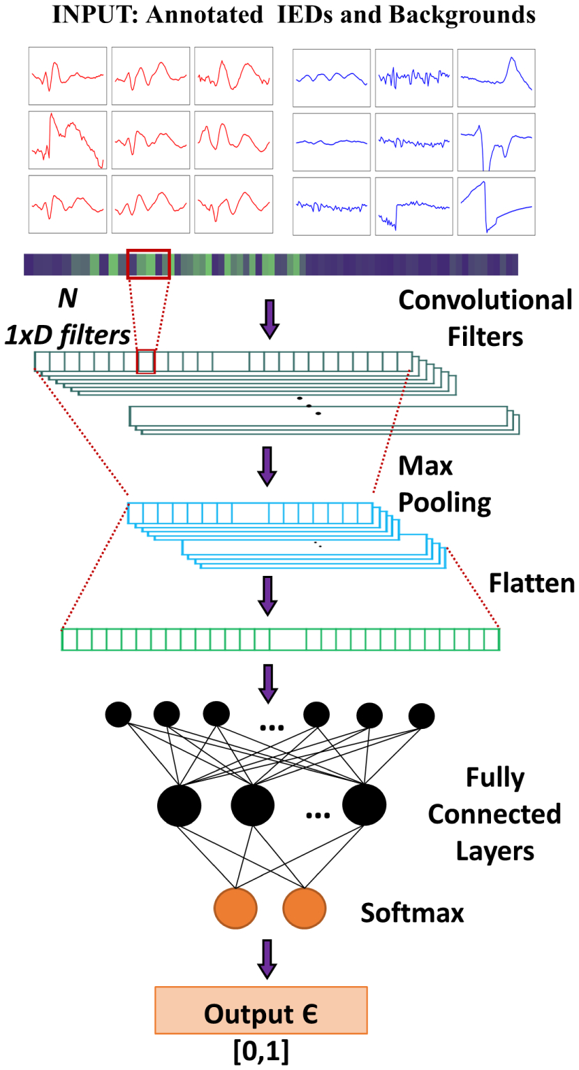
Architecture of the CNN IED detector.

While training the CNN, we applied balanced training, where the number of IEDs and background waveforms are identical. We decided to apply dropout (with a probability of 0.5) at the fully connected layer during training of the CNN, in order to prevent overfitting. We organized the training samples in mini-batches of size the same as the number of IEDs in training. We utilized the one-step background rejection technique introduced by Thomas et al.^12,18 to select suitable background waveforms for training the CNN IED detector. The hyperparameters of the CNN are optimized by applying a nested CV on the training data. During the hyperparameter optimization, the validation set in split into two: one for CNN training termination criteria and the other for hyperparameter selection.¹⁸ For each CV iteration, the network is trained until we obtain the lowest validation loss. Table 2 presents the different parameter sets optimized during the CNN training process. The CNN was implemented with Tensorflow 1.2.1²⁸ utilizing Nvidia GeForce GTX 1080 Graphical Processing Unit (GPU) on Ubuntu 16.04.

Table 2.

Parameter values evaluated for CNN optimization.

Parameters	Values/type
Number of convolution layers	1, 2, 3
Number of fully connected layers	1, 2, 3
Number of convolution filters	4, 8, 16, 32, 64
Dimension of convolution filters	1 × 3, 1 × 5, 1 × 7
Number of hidden layer neurons	16, 32, 64, 128, 256, 512
Activation function	ReLU
Dropout probability	0.5
Size of the batch processing	$\frac{n_s}{2}$
Maximum number of iterations	10,000
Optimizer	Adam
Learning rate	10−4
Measure	Cross-entropy

Notes: n_s: number of IEDs.

We design a clustering-based template library for the TM IED detector. We follow the procedures proposed by Thomas et al.¹⁹ Concretely, we apply AP²¹ in conjunction with DTW to extract the IED templates.²⁹ AP is capable of determining the cluster centers automatically based on the density of data. Also, AP in conjunction with DTW has been shown to perform better than traditional clustering methods.²⁹ Here, we employ the optimized DTW implementation by Rakthanmanon et al.²² We compute correlation²³ as the evaluation distance measure for the TM system. While extracting the template library for the TM IED detector, the Sakoe–Chiba band³⁰ of DTW was set at 0.1, the damping factor and initial priorities for AP are set as 0.9, and as the median of the similarity values, respectively. An illustration of the TM library extraction procedure is given in Fig. 2. Once the library is created, for a test 500 ms EEG segment, we compute the correlation between IED templates, and consider the minimum value across the different templates in the TM library as the TM prediction for the segment. Since we compute the correlation coefficient, the output values are in the range [0, 1], similar to that of the CNN IED detector.

Fig. 2.

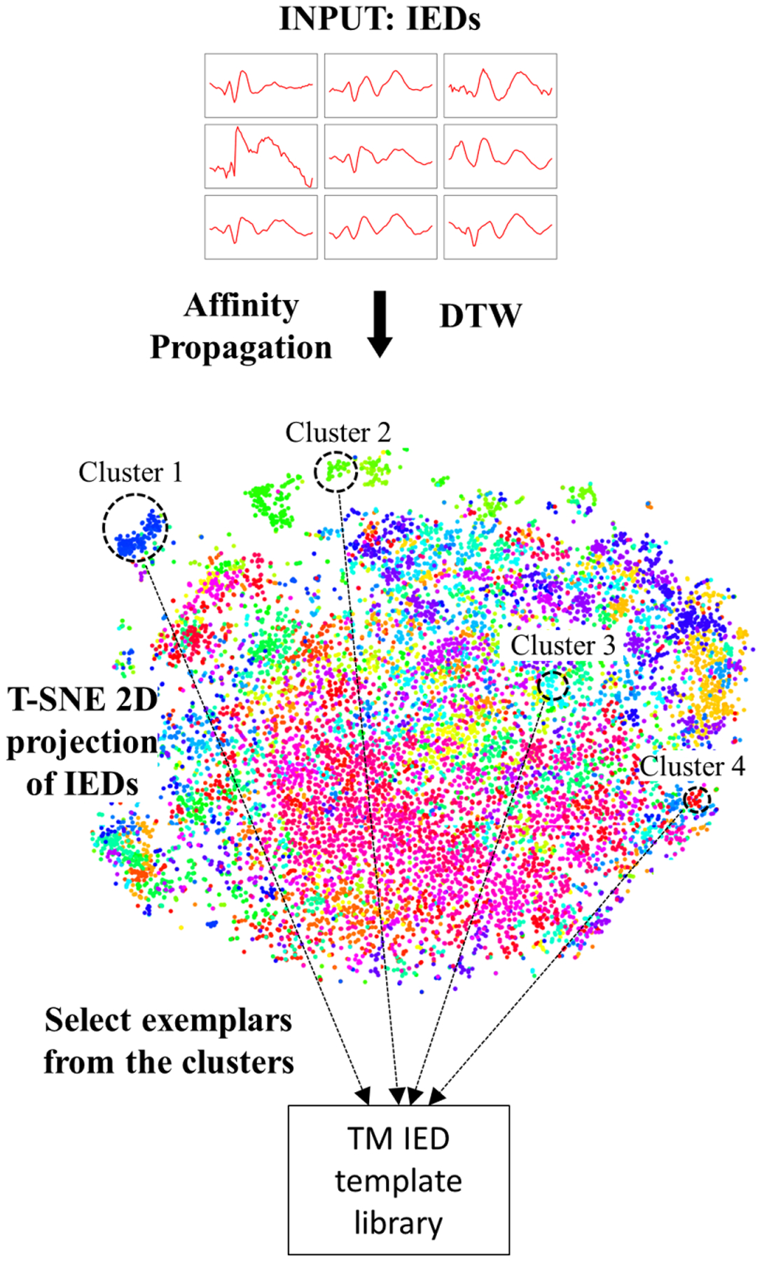
TM IED template library extraction procedure. We illustrate the different clusters generated by AP in conjunction with DTW as a 2D projection by applying t-Distributed Stochastic Neighbor Embedding (t-SNE).³¹

2.2.2. Spectral features

We investigate spectral features derived from the five standard EEG frequency bands: delta (δ, 1–4 Hz), theta (θ, 4–8 Hz), alpha (α, 8–13 Hz), beta (β, 13–30 Hz), and gamma (γ, greater than 30 Hz). Specifically, we compute relative power feature from the frequency bands:

$${\text{Relative power RP}}_f=\frac{P_f}{P_{\text{total }}},$$ (1)

where f indicate different frequency bands (f ∈ {δ, θ, α, β, γ}), P_f denotes the power in frequency band f, and P_total = P_δ + P_θ + P_α + P_β + P_γ. We compute the five features as the mean of the 19 channels of EEG. We apply this 1 × 5 feature vector as the spectral features for each EEG to perform EEG classification.

We feed the relative power values as features into an SVM with Gaussian kernel¹¹ for classification (see Fig. 3). While training the SVM, we match the number of IED EEGs and normal EEGs. The hyperparameters of SVM are optimized by applying Bayesian optimization³² with five-fold CV. Further, the SVM scores are transformed to probabilities (range [0, 1]) by applying a sigmoid function.³³

Fig. 3.

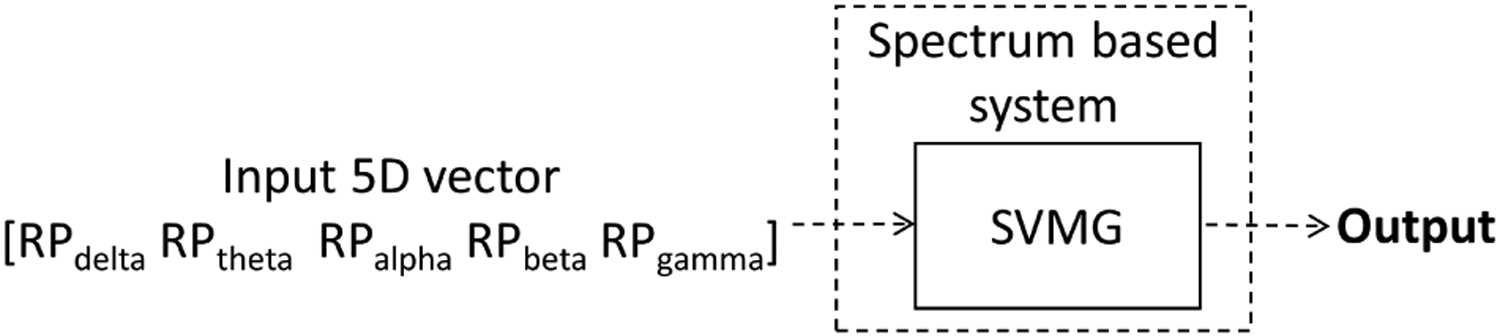
Spectral feature-based EEG classifier.

2.3. Performance assessment

2.3.1. Cross-validation on MGH dataset

First, we performed five-fold CV on the MGH dataset for evaluating the effectiveness of the three types of features: IED rates from CNN-IED and TM-IED detectors, and spectral features. The MGH dataset was divided into five folds (see Table 3), approximately matching age, gender, and annotated IED distribution in all five folds. We consider the same fold split as performed by Thomas et al.¹⁸ Moreover, we assigned EEGs from the same patient to the same fold, so that EEGs of the same patient shall never be both in the training and test set.

Table 3.

Distribution of the five folds created from the MGH dataset.

Fold number	Number of epileptic EEGs	Number of annotated IEDs	Number of nonepileptic EEGs
1	18	4077	93
2	19	3571	92
3	18	3207	92
4	19	4021	92
5	19	3288	92
Total	93	18,164	461

To investigate the EEG classification performance based on IED detection, we need to perform two steps: implement and validate the IED detectors, and implement and evaluate the EEG classifier. In the first step, we perform the training, hyperparameter optimization, and evaluation of the IED detectors (CNN and TM IED detectors). In the second step, we extract the EEG-level features, train the EEG classifier, and analyze the performance of the EEG classifier. We design an EEG classifier that contains three components: EEG classifier based on CNN IED features, EEG classifier based on TM IED detector features, and an EEG classifier based on spectral features. We evaluate these (three component classifiers, and one overall classifier) in different weighted configurations. Therefore, we need to split the data into three sets: first set for training the IED detector, second for training the EEG classifier, and finally, a separate test set. Therefore, we split the folds of the MGH dataset into three groups: three folds for IED detector/SVM training, one fold for EEG-level feature extraction/training, and one independent fold for testing. For the IED feature-based components (CNN and TM), we apply the EEG-level feature extraction/training fold for the following purposes: extract IED rates, choose the optimized CNN and TM threshold, normalize the IED feature vector, design the threshold-based EEG classifier, and finally, to optimize the weights of the ensemble EEG classifier. However, for the spectral feature-based SVM, we apply the EEG classifier training fold for optimizing the weights of the ensemble EEG classifier.

We develop the IED detectors based on the annotated MGH dataset (three training folds). Once the IED detectors are trained, the EEG-level IED rate per minute (for 100 thresholds between [0, 1]) is computed on the fourth fold, set aside for training the EEG classifier. We select the IED detector threshold that corresponds to the highest EEG classification BAC on the fourth fold. Next, we normalize the IED rates for this optimized threshold. The normalization is performed to ensure that the predictions from the three components (CNN, TM, and SVM) are in the same range. We apply normalization in two steps in order to convert the IED rates into normalized IED rates that take values in [0, 1]. First, we remove outliers; concretely, the IED rates of patients that are three or more standard deviations above the mean (of the training set) are replaced by mean + 3 × standard deviation. Next, we compute min–max normalization to the resulting IED rates x_i:

$$x_i=\frac{x_i-X_{\text{min}}}{X_{\text{max}}-X_{\text{min}}},$$ (2)

where x_i is the IED rate of a patient (after removing outliers), and X_min and X_max are the minimum and maximum values in IED rate feature vector across different patients (X). For the SVM, the outputs are already converted into the [0, 1] with a sigmoid function.³³

Once the components are ready, we evaluate the EEG classifier by applying varying weights to each individual prediction. We define weights w_CNN, w_TM, and w_S for the CNN, TM, and the spectral feature-based classifier (SVM), respectively. Next, we evaluate the possible weights (with the condition w_CNN + w_TM + w_S = 1) on the fourth fold. The best weight configuration is chosen based on AUC values on the fourth fold. Finally, the final test fold is evaluated by applying the best system configuration obtained on the training folds. In total, we have 10 (⁵C₃) sets of CNN/TM IED detectors and 20 (2 × ⁵C₃) configurations (by alternating the EEG classifier training fold and test fold) for the five-fold CV on the MGH dataset. The MGH CV procedure is illustrated in Fig. 4.

Fig. 4.

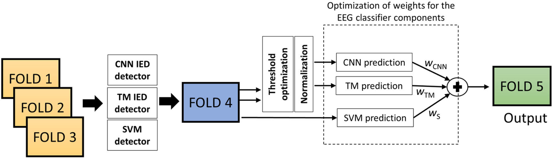
Five-fold CV evaluation on MGH dataset. Folds 1, 2, and 3 are applied to train the IED detectors and the SVM. The fold four is applied to compute the IED rates for CNN and TM, optimize the thresholds, normalize features, and develop the threshold-based EEG classifier components. The same fold is applied to optimize the weights (w_CNN, w_TM, and w_S) of the ensemble EEG classifier. Finally, the testing is performed on fold five.

2.3.2. LOSO and LOIO cross-validation

In order to perform the evaluation on the datasets, we train the IED detectors (CNN and TM) on the entire MGH dataset. We apply four folds of the MGH dataset to train the CNN IED detector and the fifth fold is applied as the validation set to determine the stopping criteria as well as the best hyperparameters. We select the CNN model that produced the lowest validation loss. Similarly, we apply all the 18,164 annotated IEDs to generate the template library. These IED detectors are kept the same during the LOSO and LOIO CV. We perform the EEG classification across multiple centers considering two scenarios:

• LOSO CV: In this scenario, we assume to have access to a sufficient number of epileptic and normal EEGs and their reports (e.g. at least 50 epileptic and 50 normal EEGs). This EEG dataset would allow us to retrain the EEG classifier, while the CNN-IED and TM-IED detectors remain fixed and are not retrained. To evaluate the performance of the proposed EEG classification system, we compute LOSO CV on data of each institution separately (with fixed CNN-IED and TM-IED detectors).

• LOIO CV: In this scenario, we directly apply the EEG classification system on a test EEG dataset, without access to EEG reports from the institution providing the data. In other words, in this case, we cannot and do not retrain the system on EEG data from that institution. In order to assess the EEG classification system for such use cases, we conduct LOIO CV, where no data is used from the target institution for training.

During the LOSO and LOIO CV evaluation process, the IED detectors (CNN and TM) are trained on three folds of the MGH dataset. The spectral features classifier (SVM) is developed by applying 50% of the training data. The remaining 50% of the data is applied as the EEG classifier training/calibration set. Similar to MGH five-fold CV, we apply this fold for designing the threshold based-IED components (CNN and TM) and optimizing the weights (w_CNN, w_TM, and w_S) of the ensemble EEG classifier (see Fig. 5). LOSO CV is performed on each dataset separately. In each iteration, one EEG of the dataset is left out as the test EEG, and the systems are trained on the remaining EEGs of that dataset (see Fig. 5). Finally, we combine the predictions of each iteration and report the results in terms of a single receiver operating characteristic (ROC). While performing the LOIO CV, we leave out the dataset from a center entirely. The EEG classification system is trained based on the data from the remaining centers (see Fig. 5). While combining the data from different centers for training, we randomly select an equal number of EEGs from each center in order to avoid any dataset bias. The number of EEGs is set as the lowest number of epileptic/normal EEGs available for any of the datasets. Also, since LTMGH EEGs are recorded with an equipment from a local manufacturer, we consider LTMGH EEGs only for testing during LOIO CV. We report standard performance metrics, including ROC curve AUC, and BAC.¹⁸ The BAC is reported for a sensitivity of 80%.

Fig. 5.

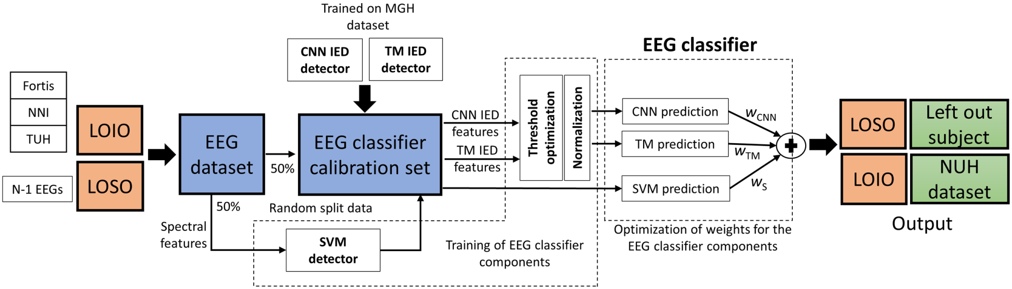
LOSO and LOIO CV methodology on the different datasets. Here, the IED detectors are trained on the three folds of the MGH dataset. The spectral feature SVM detector is trained on 50% of the training data, selected randomly. The remaining 50% of the training data is applied for EEG classifier training/calibration steps: designing the threshold based classifier for IED feature-based components (CNN and TM) and optimizing the weights (w_CNN, w_TM, and w_S) of the ensemble EEG classifier. For LOSO CV, in each iteration, one patient is evaluated by applying the system trained on the remaining EEGs. LOSO CV is performed on each dataset independently. In LOIO CV, in each iteration, the dataset from one center is evaluated from the combined dataset from other centers. In the above figure, the data from NUH is evaluated by applying the system trained on the dataset from the other centers.

3. Results

3.1. Cross-validation results on MGH dataset

We evaluated the EEG classification system on the MGH dataset by applying five-fold CV. The results are summarized in Table 4. We have evaluated eight configurations for the system weights (w_CNN, w_TM, w_S). The eight configurations are presented in Table 4, column 1. System configuration “CNN” represents EEG classifier with only CNN component, configuration “TM” represents EEG classifier with only TM component, configuration “S” represents the EEG classifier with the spectral component, configuration CNN-TM-S (equal weights) represents the classifier with equal weights of 1/3 for the three components, configuration CNN-TM-S (optimized weights) represents the classifier with the best weights optimized on the EEG classifier training set, configuration CNN-TM represents the classifier with equal weights of 1/2 for CNN and TM components, and so on.

Table 4.

Five-fold CV results on MGH dataset.

System configuration	AUC	BAC	F1-score
CNN	0.886 ± 0.09	79.9 ± 9.2%	0.646 ± 0.16
TM	0.894 ± 0.06	79.5 ± 7.2%	0.595 ± 0.13
S	0.816 ± 0.06	72.8 ± 4.9%	0.478 ± 0.08
CNN-TM-S	0.891 ± 0.06	79.8 ± 6.6%	0.614 ± 0.14
Equal Weights
CNN-TM	0.922 ± 0.06	83.0 ± 7.3%	0.692 ± 0.17
CNN-S	0.877 ± 0.06	78.2 ± 6.6%	0.575 ± 0.13
TM-S	0.859 ± 0.06	74.8 ± 6.0%	0.528 ± 0.10
CNN-TM-S	0.919 ± 0.06	83.2 ± 7.0%	0.689 ± 0.16
Optimized Weights

Notes: The results are reported as mean ±standard deviation. BAC, F1-score is reported for a sensitivity of 80%.

The proposed pipeline has achieved a mean AUC of 0.922, mean BAC of 83.0% for a configuration of CNN and TM IED detector features. The weight configuration for the CNN-TM-S (optimized weights) is presented in Fig. 6. It can be observed that w_CNN was higher in most of the cases (13/20), followed by w_TM. w_S is zero in most of the cases, indicating that the spectral features are less discriminative in comparison with IED features.

Fig. 6.

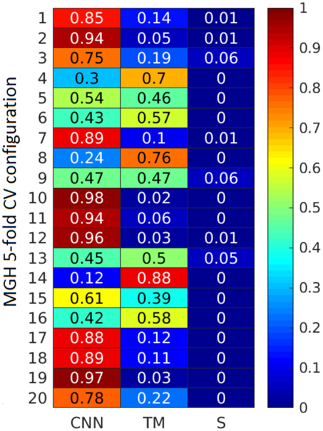
Weight configurations for the three EEG classifier components (CNN, TM, and SVM) for the 20 configurations of MGH five-fold CV.

3.2. LOSO and LOIO cross-validation results

We trained the CNN IED detector and extracted the IED template library on the entire MGH dataset. Concretely, we choose the CNN model that achieved the lowest loss value on the validation set. The network had two convolutional layers with 32 filters (dimension 1 × 5) each and one fully connected layer with 64 hidden layer neurons. We limit ourselves to a single IED detector model instead of combining models, for the sake of simplicity. We will leave the topic of model selection for future research.

We first compared the IED rates for epileptic EEGs with and without seizures. Seizures are rare during a routine EEG. However, it is a well-known fact that the IED frequency is boosted in the presence of seizures,³⁴ making it easier for classification. In Fig. 7, we plot the IED rates for a CNN threshold of 0.5 for EEGs with seizures, without seizures, and normal EEGs (NUH and TUH dataset). It can be observed that the EEGs with seizures show significantly higher IED rates in comparison with EEGs without ictal events as well as normal EEGs. Therefore, in order to prevent bias due to seizures, we further remove the EEGs whose clinical reports indicate seizure events from the NUH (31 EEGs from 31 patients), TUH (225 EEGs from 16 patients), NNI (2 EEGs from 2 patients), and Fortis (1 EEG from a patient) datasets. The three feature sets for the different datasets are illustrated in Fig. 8. The CNN feature discriminates epileptic and normal EEGs for all the datasets. The TM and spectral features are able to discriminate epileptic and normal EEGs for NUH and TUH datasets only. For NNI and LTMGH datasets, there is significant overlap between the epileptic and normal EEG features, potentially leading to more misclassifications.

Fig. 7.

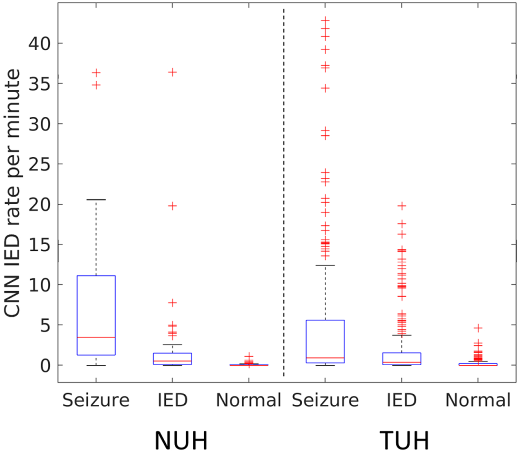
CNN IED rate per minute for epileptic EEGs with seizures, without seizures, and normal EEGs (NUH and TUH dataset). The IED rates are higher for EEGs with seizures in comparison with normal EEGs.

Fig. 8.

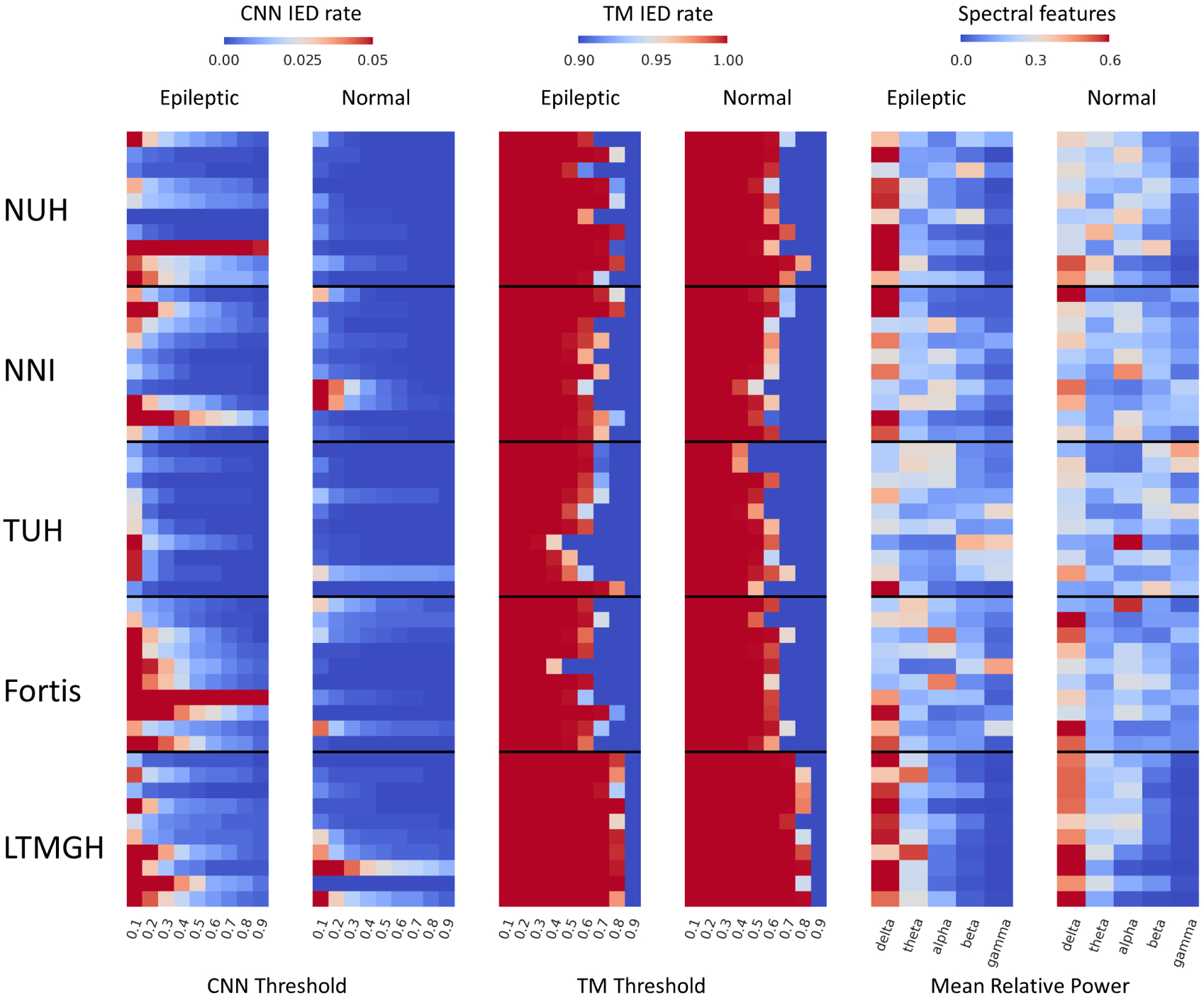
CNN, TM, and spectral features for 10 randomly selected epileptic and normal EEGs from each dataset.

The AUC and BAC values for the different datasets and three systems are summarized in Fig. 9. For the TUH dataset, since there are multiple recordings from the same patient, we perform two sets of evaluation: EEG-level evaluation (assumes each EEG as an independent observation), and patient-level evaluation (combines the features for a single patient from multiple EEGs). We consider the maximum value of individual EEG predictions while combining the different EEGs from an individual patient. While calculating the mean for AUC and BAC values, we employ the results at patient-level results for the TUH dataset.

Fig. 9.

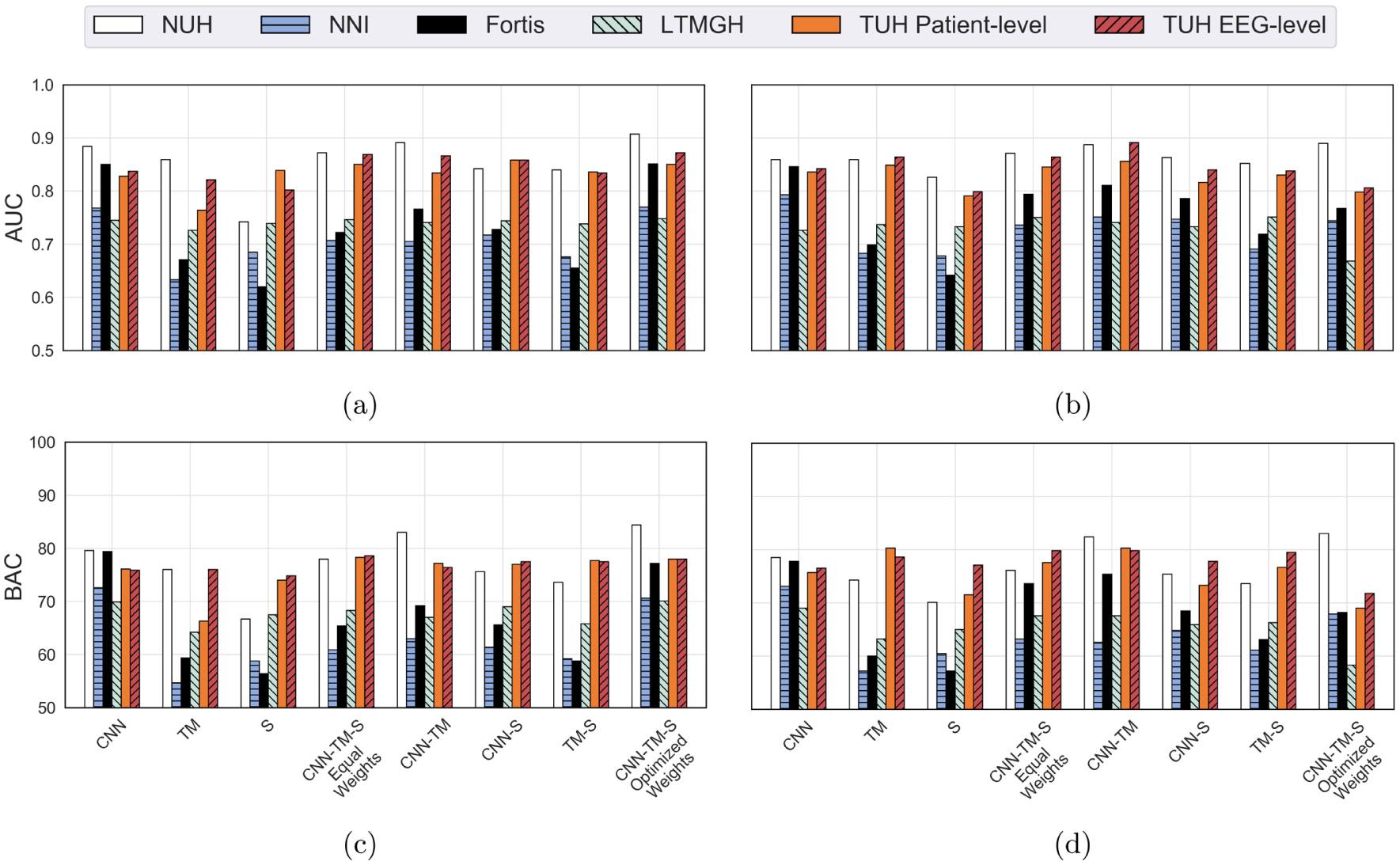
LOSO and LOIO CV results for the different datasets and system combinations (AUC and BAC): (a) LOIO AUC, (b) LOSO AUC, (c) LOIO BAC, and (d) LOSO BAC.

The results for LOSO and LOIO CV on the MGH dataset are superior to the other datasets. This is primarily due to the fact that we have trained the IED detectors on the MGH dataset. From the mean performance measures on the five datasets, it can be seen that the CNN IED detector system performed consistently over other system configurations. The TM and spectral feature-based systems performed well on selected datasets (MGH, NUH, and TUH). The mean results for LOSO and LOIO CV for the five datasets (for the different system combinations) are presented in Table 5.

Table 5.

LOSO and LOIO CV results for the different datasets (excluding MGH dataset) and different system configurations.

	LOSO CV		LOIO CV
System configuration	AUC	BAC (specificity)	AUC	BAC (specificity)
CNN	0.812 ± 0.05	74.8 ± 3.8% (69.6%)	0.815 ± 0.06	75.5 ± 4.2% (71.0%)
TM	0.766 ± 0.08	67.0 ± 9.9%(54.0%)	0.731 ± 0.09	64.1 ±8.0% (48.2%)
S	0.734 ± 0.07	62.1 ± 10.6% (44.2%)	0.725 ± 0.08	64.7 ± 7.1% (49.4%)
CNN-TM-S equal weights	0.799 ± 0.06	71.6 ± 6.1% (63.2%)	0.780 ± 0.08	70.2 ± 7.7% (60.4%)
CNN-TM	0.809 ± 0.07	73.7 ± 8.4% (67.4%)	0.788 ± 0.07	71.9 ± 8.1% (63.8%)
CNN-S	0.789 ± 0.05	69.6 ± 4.6% (59.2%)	0.778 ± 0.07	69.7 ± 6.6% (59.4%)
TM-S	0.769 ± 0.07	68.2 ± 6.7% (56.4%)	0.749 ± 0.09	67.0 ± 8.5% (54.0%)
CNN-TM-S optimized weights	0.774 ± 0.06	69.3 ± 8.8% (58.6%)	0.826 ± 0.07	76.1 ± 5.9% (72.2%)

Notes: AUC and BAC are reported as mean ± standard deviation. BAC and specificity are reported for a sensitivity of 80%.

We observe that the proposed pipeline has achieved a mean LOSO CV AUC of 0.812, LOSO CV BAC of 74.8%, LOIO CV AUC of 0.826, and LOIO CV BAC of 76.1% for the best system configuration. For LOSO CV, the CNN system performed the best, and for LOIO CV, the combination of the three systems with optimized weights performed the best. We compared the weights of the optimized combination for the LOIO evaluation and observed that the CNN system contributed the most (mean weight = 0.92), followed by TM (mean weight 0.07), and spectral feature-based system (mean weight = 0.01). Further, the mean LOIO and LOSO CV results are similar for each of the eight different configurations (see Table 5). Therefore, it seems that the proposed system generalizes well to datasets from other institutions, since training the EEG classification systems on EEG data of the target center does not improve the results much in comparison to systems that are trained on EEG data from other centers.

4. Discussion

We have developed an automated epilepsy diagnostic tool and have evaluated it on scalp EEG datasets from six different centers from the USA, Singapore, and India. The system was evaluated under two scenarios: LOSO CV (scenario where labeled EEGs from test center are available), and LOIO CV (scenario where labeled EEGs from test center are not available). We observed that the LOSO CV performance was similar to LOIO CV performance. This demonstrates that the proposed approach is generalizable as well as feasible for clinical deployment. The CNN-based system achieved a mean LOSO CV AUC of 0.812 (BAC of 74.8%) and LOIO CV AUC of 0.826 (BAC of 76.1%) on the six different datasets.

In the current literature, the IRA for IEDs and seizures is shown to be moderate to high.^35,36 In this study, the proposed system achieved LOIO CV BAC of 76%, which is in high agreement with the EEG assessment of the experts. We have summarized the literature related to EEG-level IRA in Table 6. The EEG classification performance across different centers (LOIO CV BAC) obtained in our study is superior to those reported in the literature, except for the IRA value of 80.9% reported by Jing et al.³⁵ However, this study was performed with eight experts, out of which six are from the same institution and had similar training.³⁵ Piccinelli et al. achieved a mean pairwise agreement of 88.6% across three annotators for classifying EEGs into three classes, namely, EEGs with ictal or interictal patterns, EEGs with slow waves, and normal EEGs. This study was exclusively performed for EEGs from patients with childhood idiopathic epilepsy. Moreover, ictal EEG is easier to detect than interictal EEG,³⁴ as we have also demonstrated in Sec. 3.2. Further, most studies in the literature have only been validated on datasets from a single center, while most EEG interpreters are from the same center or received similar training. Apparently, no IRA study so far considers EEG from multiple centers in different countries, similarly as the data in our study. Nevertheless such research would be quite valuable and is an interesting topic for future research.

Table 6.

EEG-level IRA literature.

Reference	IRA (percentage)	Criteria
Current study	76.1%	LOIO CV performance for classifying EEGs into two classes: EEGs with interical epileptiform patterns and normal EEGs.
Jing et al.35	80.9%	Expert agreement for classifying EEGs into two classes: EEGs with interical epileptiform patterns and normal EEGs.
Grant et al.37	77.0%	Expert agreement (mean across pair of annotators) for classifying EEGs into three classes: EEGs with ictal activity, EEGs with nonictal abnormalities, and normal EEGs.
Ding et al.38	74.0%	Expert agreement (median) across ACNS critical care EEG terminology.
Piccinelli et al.39	88.6%	Expert agreement (mean across pair of annotators) for classifying EEGs into three classes: EEGs with epileptiform patterns (ictal and interictal), EEGs with slow waves, and normal EEGs.

4.1. Comparison of system configurations

The CNN-TM combination and CNN-TM-spectral optimized weight combination performed superior to the other combinations of systems for classifying MGH EEGs. For LOIO CV, the CNN-TM-spectral optimized combination system performed the best (AUC of 0.826) with mean weights of 0.92 (CNN), 0.07 (TM), and 0.01 (spectral features), respectively. The CNN system performs well on all the datasets, whereas the TM and spectral feature-based systems yielded good performance only on certain datasets. Therefore, it is necessary to validate the diagnostic systems on multiple datasets to establish the generalizability of the system. The TM system, even though it is more explainable, is susceptible to artifacts, and therefore could potentially lead to more misclassifications. The spectral features classifier (SVM) leads to the lowest performance of the different systems. This is attributed to the difference in the EEG recording systems and as well the subject-level variance. Melnik et al. have shown that subjects could account for 32%, and EEG machines for 9% of the variance of EEG data based on a study on event-related potentials (ERPs) and steady-state visually evoked potentials (SSVEPs).⁴⁰

Moreover, we have evaluated the system on a dataset recorded from locally manufactured EEG recording equipment under non-standard conditions (LTMGH dataset). The results for LTMGH are satisfactory with an LOIO CV AUC of 0.745 (BAC of 69.9%) and LOSO CV AUC of 0.725 (BAC of 69.0%). Also, the proposed system performed consistently on the EEG recordings from diverse standard recording equipment from five centers. This implies that the performance of the proposed approach is robust toward variations introduced due to EEG recording equipment. Further, we have evaluated the performance on the public TUH Epilepsy Corpus data,⁸ freely accessible to anyone. Therefore, in the future, our results may serve as a benchmark for epileptic EEG classification.

4.2. Investigation of EEG misclassifications

We analyzed the misclassified EEGs in the LOSO CV of the CNN classifier. For MGH and NUH, the complete clinical reports were not available, and therefore a detailed investigation could not be performed. We observed that there was mention of a low occurrence of IEDs in a few clinical reports of epileptic EEGs. This accounted for 3.0% and 12.5% misclassifications for TUH and Fortis dataset, respectively.

For the normal EEG, the presence of artifacts accounted for 3.8% (NNI dataset), 4.5% (Fortis dataset), and 1.1% (LTMGH dataset) misclassifications. Similarly, for the misclassified normal EEGs, a significant percentage of patients had a recent history of epilepsy (13.4% for Fortis and 25.4% for LTMGH datasets). However, the information on whether the normal EEG is from an epileptic patient is only available for the TUH dataset. We verified whether the CNN classifier is able to distinguish normal EEGs from epileptic patients versus normal EEGs from nonepileptic patients. We obtained a classification AUC of 0.536, indicating there is no significant difference between the EEGs in terms of IEDs. Also, it is well understood that the EEGs from patients with epilepsy do not have to have IEDs. Moreover, annotating IEDs by visual inspection is inherently subjective.^4,41 Therefore, an interesting direction for future research is to explore additional EEG features beyond IEDs and spectral information, e.g. interictal networks inferred from scalp EEG,¹⁰ for distinguishing epileptic from nonepileptic EEGs.

4.3. Comparison to the state-of-the-art

We achieved five-fold CV mean AUC of 0.886 on the MGH dataset for the CNN system (see Table 4). This is superior to our previous results¹² (AUC of 0.87) and better than the results reported by Jing et al.¹³ (AUC of 0.847) even though Jing et al. had performed the evaluation on a larger EEG dataset from MGH. We have evaluated the proposed pipeline across six institutions. The EEGs in the different institutions were annotated by experts belonging to the respective centers. This makes our results more robust and reliable, in comparison with the studies performed on datasets from a single center.^10,12,13 Furthermore, we have evaluated entire EEGs for analysis rather than hand-picked EEG segments. Therefore, our assessment more closely resembles real-life clinical settings.

The proposed CNN system approximately takes slightly more than a second (on a CPU+GPU system) for evaluating a single 30-min 19-channel routine EEG recording sampled at 128 Hz (excluding the time taken to load the data and model). The detailed time profiling of the CNN system is presented in Table 7. An expert takes approximately 10 min to review a 30-min routine EEG.¹⁸ Therefore, the CNN system can be operated in real time, thereby improving the efficiency of epilepsy diagnosis. The evaluation was performed with an Intel (R) Xeon(R) CPU E5–2630 v4 @2.2 GHz CPU, Nvidia GeForce GTX 1080 GPU, in Python v3.5. The proposed system could be applied to EEG with any arbitrary number of electrodes. This is due to the fact that the IED detectors are trained at the channel level. This would be beneficial in the context of wearable epilepsy diagnostic devices.

Table 7.

Time cost of evaluation of a 19-channel 30-min EEG recording (128 Hz).

Task	Time cost (s)
EEG loading from hard disk	1.1 ± 0.13
CNN model loading from hard disk	4.1 ± 0.12
Preprocessing	0.74 ± 0.07
CNN evaluation (CPU + GPU)	0.45 ± 0.01
CNN evaluation (CPU only)	8.4 ± 0.11
EEG feature extraction and evaluation	Less than 0.02

Notes: Time is reported as mean ± standard deviation.

This study has the following limitations. First, the proposed pipeline leverages on the performance of the CNN IED detector. Therefore, the system performance could be further improved by training the IED detector with more annotated interictal patterns. Also, the false positives in IED detection could be improved by applying a sophisticated artifact rejection system. Second, we have predominantly evaluated adults EEGs (age > 20 years). Aanestad et al. have shown that a system should operate at an age-dependent threshold for epilepsy diagnostics, as IEDs have age-dependent characteristics.⁴² Consequently, a separate study is required to evaluate the performance on EEGs of patients younger than 20 years. Third, we have applied the CAR montage for the evaluation of IEDs. However, in a typical clinical setting, multiple montages are applied by clinicians to make annotate EEGs. Therefore, it would be beneficial to consider multiple montages in the machine learning pipeline. We will explore combinations of montages in the future.

5. Conclusion and Future work

We have developed an efficient, automated, and generalized epileptic EEG diagnostic system based on interictal pattern detection. The proposed system was evaluated cross-institutionally on data from six different centers and achieved a mean LOSO CV AUC of 0.812 (BAC of 74.8%) and LOIO CV AUC of 0.826 (BAC of 76.1%). The proposed EEG classification system may thus be a practical tool to aid the neurologists for accelerated review of epileptic EEGs.

Acronyms.

EEG

Electroencephalogram

IED

Interictal epileptiform discharge

CNN

Convolutional neural network

TM

Template matching

CV

Cross-validation

AUC

Area under curve

BAC

Balanced accuracy

LOIO

Leave-one-institution-out

LOSO

Leave-one-subject-out

IRA

Interrater agreement

ROC

Receiver operating characteristics

SVM

Support vector machine

1D/2D

One-/two-dimensional

AP

Affinity propagation

DTW

Dynamic time warping

MGH

Massachusetts General Hospital

TUH

Temple University Hospital

NUH

National University Hospital

NNI

National Neuroscience Institute

LTMGH

Lokmanya Tilak Municipal General Hospital

ReLU

Rectified linear units

RP

Relative power

References

- 1.Thijs RD, Surges R, O’Brien TJ and Sander JW, Epilepsy in adults, Lancet 393 (2019) 689–701. [DOI] [PubMed] [Google Scholar]
- 2.Adeli H, Zhou Z and Dadmehr N, Analysis of EEG records in an epileptic patient using wavelet transform, J. Neurosci. Methods 123(1) (2003) 69–87. [DOI] [PubMed] [Google Scholar]
- 3.Frauscher B and Gotman J, Sleep, oscillations, interictal discharges, and seizures in human focal epilepsy, Neurobiol. Dis 127 (2019) 545–553. [DOI] [PubMed] [Google Scholar]
- 4.Pillai J and Sperling MR, Interictal EEG and the diagnosis of epilepsy, Epilepsia 47 (2006) 14–22. [DOI] [PubMed] [Google Scholar]
- 5.Fountain NB and Freeman JM, EEG is an essential clinical tool: Pro and con, Epilepsia 47 (2006) 23–25. [DOI] [PubMed] [Google Scholar]
- 6.Roy S, Kiral-Kornek I and Harrer S, Chrononet: A deep recurrent neural network for abnormal EEG identification, in Conf. Artificial Intelligence in Medicine in Europe (Springer, 2019), pp. 47–56. [Google Scholar]
- 7.López S, Obeid I and Picone J, Automated interpretation of abnormal adult electroencephalograms, MS thesis, Temple University; (2017). [Google Scholar]
- 8.Obeid I and Picone J, The temple university hospital EEG data corpus, Front. Neurosci 10 (2016) 196. [DOI] [PMC free article] [PubMed] [Google Scholar]
- 9.Gemein LA, Schirrmeister RT, Chrabaszcz P, Wilson D, Boedecker J, Schulze-Bonhage A, Hutter F and Ball T, Machine-learning-based diagnostics of EEG pathology, NeuroImage 220 (2020) 117021. [DOI] [PubMed] [Google Scholar]
- 10.Schmidt H, Woldman W, Goodfellow M, Chowdhury FA, Koutroumanidis M, Jewell S, Richardson MP and Terry JR, A computational biomarker of idiopathic generalized epilepsy from resting state EEG, Epilepsia 57(10) (2016) e200–e204. [DOI] [PMC free article] [PubMed] [Google Scholar]
- 11.Hearst MA, Dumais ST, Osuna E, Platt J and Scholkopf B, Support vector machines, IEEE Intell. Syst. Appl 13(4) (1998) 18–28. [Google Scholar]
- 12.Thomas J, Comoretto L, Jin J, Dauwels J, Cash SS and Westover MB, EEG classification via convolutional neural network-based interictal epileptiform event detection, in 2018 40th Annual Int. Conf. IEEE Engineering in Medicine and Biology Society (EMBC) (IEEE, 2018), pp. 3148–3151. [DOI] [PMC free article] [PubMed] [Google Scholar]
- 13.Jing J, Sun H, Kim JA, Herlopian A, Karakis I, Ng M, Halford JJ, Maus D, Chan F, Dolatshahi M et al. , Development of expert-level automated detection of epileptiform discharges during electroencephalogram interpretation, JAMA Neurol. 77(1) (2020) 103–108. [DOI] [PMC free article] [PubMed] [Google Scholar]
- 14.Acharya UR, Oh SL, Hagiwara Y, Tan JH and Adeli H, Deep convolutional neural network for the automated detection and diagnosis of seizure using EEG signals, Comput. Biol. Med 100 (2018) 270–278. [DOI] [PubMed] [Google Scholar]
- 15.Lu D and Triesch J, Residual deep convolutional neural network for EEG signal classification in epilepsy, arXiv:1903.08100. [Google Scholar]
- 16.Andrzejak RG, Lehnertz K, Mormann F, Rieke C, David P and Elger CE, Indications of nonlinear deterministic and finite-dimensional structures in time series of brain electrical activity: Dependence on recording region and brain state, Phys. Rev. E 64(6) (2001) 061907. [DOI] [PubMed] [Google Scholar]
- 17.Andrzejak RG, Schindler K and Rummel C, Nonrandomness, nonlinear dependence, and nonstationarity of electroencephalographic recordings from epilepsy patients, Phys. Rev. E 86(4) (2012) 046206. [DOI] [PubMed] [Google Scholar]
- 18.Thomas J, Jin J, Thangavel P, Bagheri E, Yuvaraj R, Dauwels J, Rathakrishnan R, Halford JJ, Cash SS and Westover B, Automated detection of interictal epileptiform discharges from scalp electroencephalograms by convolutional neural networks, Int. J. Neural Syst 30(11) (2020) 2050030. [DOI] [PMC free article] [PubMed] [Google Scholar]
- 19.Thomas J, Jin J, Dauwels J, Cash SS and Westover MB, Automated epileptiform spike detection via affinity propagation-based template matching, in 2017 39th Annual Int. Conf. IEEE Engineering in Medicine and Biology Society (EMBC) (IEEE, 2017), pp. 3057–3060. [DOI] [PMC free article] [PubMed] [Google Scholar]
- 20.Thomas J, Epilepsy diagnosis from scalp EEG: A machine learning approach, Ph.D. thesis, Nanyang Technological University; (2019). [Google Scholar]
- 21.Frey BJ and Dueck D, Clustering by passing messages between data points, Science 315(5814) (2007) 972–976. [DOI] [PubMed] [Google Scholar]
- 22.Rakthanmanon T, Campana B, Mueen A, Batista G, Westover B, Zhu Q, Zakaria J and Keogh E, Searching and mining trillions of time series subsequences under dynamic time warping, in Proc. 18th ACM SIGKDD Int. Conf. Knowledge Discovery and Data Mining (Association for Computing Machinery, 2012), pp. 262–270. [DOI] [PMC free article] [PubMed] [Google Scholar]
- 23.Sedgwick P, Pearson’s correlation coefficient, Bmj 345 (2012) e4483. [Google Scholar]
- 24.Larsson PG and Kostov H, Lower frequency variability in the alpha activity in EEG among patients with epilepsy, Clin. Neurophysiol 116(11) (2005) 2701–2706. [DOI] [PubMed] [Google Scholar]
- 25.Thomas J, Maszczyk T, Sinha N, Kluge T and Dauwels J, Deep learning-based classification for brain-computer interfaces, in 2017 IEEE Int. Conf. Systems, Man, and Cybernetics (SMC) (IEEE, 2017), pp. 234–239. [Google Scholar]
- 26.Jing J, Dauwels J, Rakthanmanon T, Keogh E, Cash S and Westover M, Rapid annotation of interictal epileptiform discharges via template matching under dynamic time warping, J. Neurosci. Methods 274 (2016) 179–190. [DOI] [PMC free article] [PubMed] [Google Scholar]
- 27.Veloso L, McHugh J, von Weltin E, Lopez S, Obeid I and Picone J, Big data resources for EEGs: Enabling deep learning research, 2017 IEEE Signal Processing in Medicine and Biology Symp. (SPMB) (IEEE, 2017), pp. 1–3. [Google Scholar]
- 28.Abadi M, Agarwal A, Barham P, Brevdo E, Chen Z, Citro C, Corrado GS, Davis A, Dean J, Devin M et al. , Tensorflow: Large-scale machine learning on heterogeneous distributed systems, arXiv:1603.04467. [Google Scholar]
- 29.Thomas J, Jin J, Dauwels J, Cash SS and Westover MB, Clustering of interictal spikes by dynamic time warping and affinity propagation, 2016 IEEE Int. Conf. Acoustics, Speech and Signal Processing (ICASSP) (IEEE, 2016), pp. 749–753. [DOI] [PMC free article] [PubMed] [Google Scholar]
- 30.Sakoe H and Chiba S, Dynamic programming algorithm optimization for spoken word recognition, IEEE Trans. Acoust. Speech Signal Process 26(1) (1978) 43–49. [Google Scholar]
- 31.Van der Maaten L and Hinton G, Visualizing data using t-SNE, J. Mach. Learn. Res 9(2579–2605) (2008) 85. [Google Scholar]
- 32.Martinez-Cantin R, Bayesopt: A Bayesian optimization library for nonlinear optimization, experimental design and bandits, J. Mach. Learn. Res 15(1) (2014) 3735–3739. [Google Scholar]
- 33.Platt J et al. , Probabilistic outputs for support vector machines and comparisons to regularized likelihood methods, Advances in Large Margin Classifiers, Vol. 10, No. 3 (Cambridge, MA, 1999), pp. 61–74. [Google Scholar]
- 34.Karoly PJ, Freestone DR, Boston R, Grayden DB, Himes D, Leyde K, Seneviratne U, Berkovic S, O’Brien T and Cook MJ, Interictal spikes and epileptic seizures: Their relationship and underlying rhythmicity, Brain 139 (2016) 1066–1078. [DOI] [PubMed] [Google Scholar]
- 35.Jing J, Herlopian A, Karakis I, Ng M, Halford JJ, Lam A, Maus D, Chan F, Dolatshahi M, Muniz CF et al. , Interrater reliability of experts in identifying interictal epileptiform discharges in electroencephalograms, JAMA Neurol. 77(1) (2020) 49–57. [DOI] [PMC free article] [PubMed] [Google Scholar]
- 36.Halford J, Shiau D, Desrochers J, Kolls B, Dean B, Waters C, Azar N, Haas K, Kutluay E, Martz G et al. , Inter-rater agreement on identification of electrographic seizures and periodic discharges in ICU EEG recordings, Clin. Neurophysiol 126(9) (2015) 1661–1669. [DOI] [PMC free article] [PubMed] [Google Scholar]
- 37.Grant AC, Abdel-Baki SG, Weedon J, Arnedo V, Chari G, Koziorynska E, Lush-bough C, Maus D, McSween T, Mortati KA et al. , EEG interpretation reliability and interpreter confidence: A large single-center study, Epilepsy Behav. 32 (2014) 102–107. [DOI] [PMC free article] [PubMed] [Google Scholar]
- 38.Ding JZ, Mallick R, Carpentier J, McBain K, Gaspard N, Westover MB and Fantaneanu TA, Resident training and interrater agreements using the ACNS critical care EEG terminology, Seizure 66 (2019) 76–80. [DOI] [PMC free article] [PubMed] [Google Scholar]
- 39.Piccinelli P, Viri M, Zucca C, Borgatti R, Romeo A, Giordano L, Balottin U and Beghi E, Inter-rater reliability of the EEG reading in patients with childhood idiopathic epilepsy, Epilepsy Res. 66(1–3) (2005) 195–198. [DOI] [PubMed] [Google Scholar]
- 40.Melnik A, Legkov P, Izdebski K, Kärcher SM, Hairston WD, Ferris DP and König P, Systems, subjects, sessions: To what extent do these factors influence EEG data? Front. Hum. Neurosci 11 (2017) 150. [DOI] [PMC free article] [PubMed] [Google Scholar]
- 41.Smith S, EEG in the diagnosis, classification, and management of patients with epilepsy, J. Neurol. Neurosurg. Psychiatry 76(Suppl. 2) (2005) ii2–ii7. [DOI] [PMC free article] [PubMed] [Google Scholar]
- 42.Aanestad E, Gilhus NE and Brogger J, Interictal epileptiform discharges vary across age groups, Clin. Neurophysiol 131(1) (2020) 25–33. [DOI] [PubMed] [Google Scholar]