Fully Automated 3D Vestibular Schwannoma Segmentation with and without Gadolinium-based Contrast Material: A Multicenter, Multivendor Study

Abstract

Purpose

To develop automated vestibular schwannoma measurements on contrast-enhanced T1- and T2-weighted MRI scans.

Materials and Methods

MRI data from 214 patients in 37 different centers were retrospectively analyzed between 2020 and 2021. Patients with hearing loss (134 positive for vestibular schwannoma [mean age ± SD, 54 years ± 12;64 men] and 80 negative for vestibular schwannoma) were randomly assigned to a training and validation set and to an independent test set. A convolutional neural network (CNN) was trained using fivefold cross-validation for two models (T1 and T2). Quantitative analysis, including Dice index, Hausdorff distance, surface-to-surface distance (S2S), and relative volume error, was used to compare the computer and the human delineations. An observer study was performed in which two experienced physicians evaluated both delineations.

Results

The T1-weighted model showed state-of-the-art performance, with a mean S2S distance of less than 0.6 mm for the whole tumor and the intrameatal and extrameatal tumor parts. The whole tumor Dice index and Hausdorff distance were 0.92 and 2.1 mm in the independent test set, respectively. T2-weighted images had a mean S2S distance less than 0.6 mm for the whole tumor and the intrameatal and extrameatal tumor parts. The whole tumor Dice index and Hausdorff distance were 0.87 and 1.5 mm in the independent test set. The observer study indicated that the tool was similar to human delineations in 85%–92% of cases.

Conclusion

The CNN model detected and delineated vestibular schwannomas accurately on contrast-enhanced T1- and T2-weighted MRI scans and distinguished the clinically relevant difference between intrameatal and extrameatal tumor parts.

Keywords: MRI, Ear, Nose, and Throat, Skull Base, Segmentation, Convolutional Neural Network (CNN), Deep Learning Algorithms, Machine Learning Algorithms

Supplemental material is available for this article.

© RSNA, 2022

Summary

Automated measurement of vestibular schwannoma using a convolutional model in a multicenter setting on contrast-enhanced T1- and T2-weighted MRI scans was accurate and similar to human measurements.

Key Points

• ■ The convolutional neural network detected and delineated vestibular schwannomas accurately on MRI scans, with mean surface-to-surface (S2S) distances less than 0.6 mm.

• ■ Whole tumor volume, as well as intrameatal and extrameatal volume, could be measured on T1-weighted and T2-weighted MRI scans.

• ■ The multicenter, multivendor design enabled a robust model with mean S2S less than 0.4 mm on an external publicly available dataset.

• ■ The CNN detected tumors with 100% sensitivity and 99.1% specificity for the validation set and 100% sensitivity and 100% specificity for the test set.

Introduction

Vestibular schwannomas are rare, benign intracranial tumors arising from the neurilemma of the vestibular nerve. Initial symptoms usually comprise hearing loss, tinnitus, and balance disturbance. Approximately 60% of tumors show no or minimal progression over time, and 40% either are very large at presentation or show progression during follow-up (1). Small- to medium-sized tumors are not life-threatening and are generally conservatively managed, at least initially, using surveillance with repeated MRI examinations. Conversely, patients with large tumors at presentation or with tumors that progress during follow-up may need intervention through radiation therapy or surgery. There are no reliable predictors for tumor progression.

Tumor progression is determined according to the extrameatal manual diameter measurements at subsequent MRI examinations (2). However, these two-dimensional (2D) measurements have considerable error, resulting in inter- and intraannotator differences of 10%–40% (3–5). The more accurate three-dimensional (3D) volume measurements have not been widely applied in clinical practice because these measurements are time-consuming (3–6).

To address this problem, several automated segmentation tools have been developed (7–9). The reported tools were trained for volume measurement of vestibular schwannoma with gadolinium-enhanced T1-weighted MRI and sometimes additional T2-weighted MRI. These tools are increasingly based on deep learning methods, which yield state-of-the-art performance in many vision tasks, including medical image segmentation. Deep convolutional neural networks (CNNs), particular the U-Net architecture, can reach expert-level performance in various organ segmentation tasks from clinical MRI (8). Although many variants of the U-Net have been proposed and demonstrated task-specific improvements, recent insights suggest that rather than the architecture, careful selection of the hyperparameters and training strategy can have an important effect on performance (9). The no-new-U-Net framework, abbreviated nnU-Net, indeed demonstrated this for several organs and imaging modalities (10,11). As such, we propose application of nnU-Net to address vestibular schwannoma segmentation in our clinical setting.

This study aimed to develop a deep learning CNN model to automatically detect and segment vestibular schwannoma in 3D from T2-weighted and gadolinium-enhanced T1-weighted MRI scans, acquired from multiple centers using different MRI scanners and scan protocols. We additionally carried out a carefully designed observer study, based on the concept that the radiologists’ visual observation of the segmentation results can be a direct, important evaluation of segmentation quality. In addition to conventional metrics, the observer study highlights the applicability of our model in a clinical setting.

Materials and Methods

This retrospective study was performed at the Leiden University Medical Center, a tertiary referral center for vestibular schwannoma in 2020–2021. The institutional review board approved the study protocol (G19.115) and waived the obligation to obtain informed consent.

Patients and Data

In total, 214 patients who underwent MRI because of hearing loss were included in the study, with 134 patients who were vestibular schwannoma positive (mean age, 54 years ± 12 [SD]; 64 men) and 80 who were vestibular schwannoma negative. Selection of patients with vestibular schwannoma included a wide spectrum of patient and tumor characteristics, such as patient age, sex, tumor size, and tumor consistency. All positive patients were adults with a unilateral vestibular schwannoma and at least one gadolinium-enhanced T1-weighted MRI examination. High-resolution T2-weighted images were available in 112 patients. MRI scans obtained after surgery or irradiation were excluded. Available MRI examinations were originally performed in 37 different hospitals with 12 different MRI scanners from three major MRI vendors. The MRI scans of negative cases, included to optimize detection performance, were solely acquired at the Leiden University Medical Center in adult patients with hearing loss before cochlear implantation and provided no demographic data because of previous anonymization. Patients’ characteristics and technical information are shown in Tables 1 and 2, respectively.

Table 1:

Characteristics of Patients with Vestibular Schwannoma

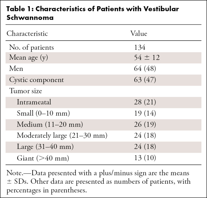
Table 2:

Technical Information of Patients with Vestibular Schwannoma

In positive cases, the intra- and extrameatal components (2) and the whole tumor were manually delineated by two annotators independently (O.M.N., a physician with 3 years of experience, and S.R.R., a technical physician with 2 years of experience) with gadolinium-enhanced T1-weighted MRI, supervised and, when necessary, corrected by a senior head-and-neck radiologist (B.M.V.). Two senior radiologists (M.C.K. and B.M.V., with 18 and 21 years of experience) trained both annotators. Delineation was performed using Vitrea software, version 7.14.2.227 (Vital Images). The delineation was automatically propagated to T2-weighted MRI after rigid image registration using elastix software (12,13). The complete dataset was split into a training and validation set (80% from 26 centers) and an independent test set (20% from 11 different centers) on which the model was not trained; see Figure 1 for details. This was done to mimic clinical deployment, in which new cases may be slightly different from the data seen in the training phase and possibly bear an unknown distribution shift (14).

Figure 1:

Flowchart of data. Patients were randomly assigned to the training and validation set (80%) and the independent test set (20%). Positive cases were randomly assigned on the basis of the hospital where the scan was acquired, so the independent test set contained data of 11 hospitals that were not used to train the algorithm. For training and validation, fivefold cross-validation was used. The mean of the five models is the ensemble model. This ensemble model was evaluated in the independent test set.

Furthermore, the publicly available dataset by Shapey et al (15) was used as additional external test of the contrast-enhanced T1-weighted model (n = 242). This dataset contained 47 postsurgery scans, which were omitted from the analysis.

CNN Architecture and Training

NnU-Net is a deep learning–based segmentation method that automatically selects one of three network architectures, includes preprocessing and postprocessing methods, and performs automatic tuning of hyperparameters (10). In this study, a 3D U-Net with five encoder and decoder layers was selected, using randomly cropped 3D image patches of size 320 × 320 × 20 voxels as network input during training. The network was trained as a multiclass segmentation task to automatically segment both the intra- and extrameatal component of the tumor. Two 3D nnU-Nets were trained (one for contrast-enhanced T1-weighted MRI and one for T2-weighted MRI) from scratch with He initialization. Fivefold cross-validation was used, generating five models that were merged by averaging the softmax scores. To deal with multicenter settings, z-scoring normalization was performed to each image independently. All the training images were then resampled to the median spacing of the training dataset using third-order spline interpolation. Training was performed on an NVIDIA Tesla V100 graphics processing unit (NVIDIA) with 16-GB memory using the PyTorch (version 1.7.1) library.

Observer Study

An observer study was performed to test whether the CNN could perform as well as human delineation on contrast-enhanced T1-weighted images. The T1-weighted annotations were propagated to T2-weighted MRI; therefore, the observer study was conducted only for the T1-weighted images. A user interface was created (Fig 2), showing a gadolinium-enhanced T1-weighted image and the registered T2-weighted image in the top row and the human and automatic delineation in random order on the bottom row, projected on the gadolinium-enhanced T1-weighted MRI scan. Observers could scroll through the MRI scan, manually adjust its brightness and contrast, and toggle the segmentations on and off for optimal assessment. The observers were a head-and-neck radiologist (B.M.V.) and a skull-base otorhinolaryngologist (E.F.H., with 18 years of experience), blinded to case information and delineation type (human or automated). The observers were asked to rate and compare the two delineations by answering two separate questions about the intra- and extrameatal part and the whole tumor: (a) Which delineation is better (annotation 1, annotation 2, or similar) and (b) is the annotation quality satisfactory (yes or no). In a consensus meeting, cases in which observers did not agree were discussed. The consensus results are presented in the section on outcomes of observer study.

Figure 2:

Observer study interface. The top row shows the clean, gadolinium-enhanced T1-weighted MRI and T2-weighted MRI scans. The bottom row shows the convolutional neural network and human annotations, randomized to the left and the right pane, respectively. The multiple-choice questions for each observer are shown at the right side of the interface. The observers could also add free-text comments.

Testing and Statistical Analysis

All test images were resampled in the same way as the training data, and a sliding window approach was used to predict images with a window size of 320 × 320 × 10 voxels, which is the same as the network’s input size. The step size is half of the window size, and a Gaussian weighted function was applied in aggregating the predictions. To eliminate false detection, connected component-based postprocessing was performed. Only the largest connected component in the predictions was kept. Tumor detection by the CNN was defined as at least 1 voxel being detected. The performance was evaluated using the Dice index (measuring overlap of the delineations), 95th percentile Hausdorff distance (indicating the maximum distance between delineations), surface-to-surface (S2S) distance (indicating the mean distance between delineations), and the relative volume error (RVE) (indicating the difference in volume in percentage). One of the annotator’s (O.M.N., annotator 1) delineations were used for training and quantitative evaluation. The results were plotted in box-and-whisker plots. Furthermore, interannotator variability was investigated. Differences between the prediction performance of each annotator and the interannotator variabilities were tested using the Wilcoxon signed rank test. In addition, a post hoc analysis of T1-model performance was conducted with respect to tumor size, according to the classification by Kanzaki et al (2). To avoid group sizes that were too small per category, the validation and test set were pooled and a Kruskal-Wallis test was performed. P values less than .05 were considered to indicate statistically significant differences. Observer agreement before the consensus meeting on satisfactory degree for segmentation and human delineation was expressed as percentage agreement. All analyses were performed in Python (version 3.8.2) with NumPy (version 1.20.2), SciPy (version 1.3.3), and the sklearn (version 0.23.2) library.

Results

The CNN detected tumors with 100% sensitivity and 99.1% specificity for the validation set and 100% sensitivity and 100% specificity for the test set. The algorithm calculated the segmentation with a median runtime of 78 seconds per patient.

Performance with Contrast-enhanced T1-weighted MRI

The results of the CNN on contrast-enhanced T1-weighted MRI scans are shown in Table 3 and Figure 3A. S2S distance of the whole tumor was 0.31 mm ± 0.36 (SD) in the validation set and 0.47 mm ± 0.67 in the independent test set. These S2S distances are around the in-plane voxel size and lower than the section thickness. The whole tumor Hausdorff distance in the independent test set was 2.10 mm ± 3.34; it was 1.34 mm ± 0.84 and 2.18 mm ± 3.43 in the intra- and extrameatal parts, respectively. All the median Hausdorff distances were below the 2-mm threshold, which is often used in clinical practice to define 2D growth (1). T1 model performance on the independent test set was similar to the results in the validation set, indicating robust external validity. The independent test set had higher mean Hausdorff properties than the median because of two outliers (cystic tumor) in the test set that influenced the Hausdorff distance and its SD. Dice indexes for the whole tumor were above 0.91 ± 0.10 and 0.92 ± 0.05 in both sets, and RVE was 7.6% ± 4.9 and 10.2% ± 9.1, with lower values for the intra- and extrameatal parts of the tumor due to the sensitivity of Dice and RVE to small volumes. Figure 4 shows examples of the T1 model compared with annotator 1.

Table 3:

Quantitative Results of Contrast-enhanced T1-weighted Model

Figure 3:

Quantitative boxplots of convolutional neural network tumor segmentation performance. The Dice 95% Hausdorff (Hausdorff95) distance and surface-to-surface distance (S2S) measures are shown from left to right. (A) Results of the contrast-enhanced T1-weighted model. (B) Results of the T2-weighted model. Validation set results are shown in sky blue and independent test set results in dark blue. Box extends from the first to third quartile, with line at the median. Whiskers extend from the box 1.5 times the interquartile range. Data points outside the whiskers were plotted individually.

Figure 4:

Examples of cystic, large, and small vestibular schwannoma whole tumor annotations, including the separation between the intra- and extrameatal tumor parts, of contrast-enhanced T1-weighted MRI scans. The top row shows the convolutional neural network (CNN) predictions in red, and the bottom row shows the delineation of annotator 1 in green. The first, fourth, and fifth tumors are potentially hard to delineate for the CNN because of the large peripheral cystic tumor parts. The Dice scores of these patients were 0.96, 0.96, 0.91, 0.93, and 0.72, respectively, and the surface-to-surface distances were 0.39 mm, 0.21 mm, 0.24 mm, 0.35 mm, and 3.44 mm, respectively.

The CNN model, when applied to the publicly available dataset of Shapey et al (15), performed at the same level as with the independent test set, with a mean Dice index of 0.88 ± 0.04, a mean Hausdorff distance of 1.31 mm ± 0.22, a mean S2S distance of 0.39 mm ± 0.12, and an RVE of 26% ± 11.9.

Performance with T2-weighted MRI

The results of the whole tumor and the intra- and extrameatal parts are summarized in Table 4 and Figure 3B. S2S distances ranged between 0.46 mm ± 0.28 and 1.00 mm ± 3.75 for all tumor parts in both datasets. Hausdorff distance of the whole tumor in the validation set was 3.12 mm ± 9.28, with a smaller value in the independent test set (1.52 mm ± 0.76). Whole tumor Dice indexes were 0.82 ± 0.19 and 0.87 ± 0.06, and RVE values ranged from 12.1% ± 10.8 and 24.5% ± 98.8 in both datasets. Intrameatal tumors had worse Dice indexes (0.69 ± 0.23 and 0.74 ± 0.08) and RVE (14.5% ± 18.7 and 12.6% ± 21.2), likely due to the low contrast between the tumor and adjacent petrous bone on T2-weighted images. Overall T2 performance was slightly degraded compared with postcontrast T1. However, S2S distances below 1 mm indicate acceptable performance.

Table 4:

Quantitative Results of T2-weighted Model

Interannotator Variability

Comparisons between the T1-weighted model and the two annotators and between the two annotators are shown in Table 5 and Figure 5. The comparison between both annotators shows the whole tumor interannotator variability, resulting in a Dice index around 0.91 and RVE of 7%–9%. When the model was compared with each annotator in both datasets, S2S distances were similar and below 0.5 mm. The model was trained on annotator 1, but the results compared with annotator 2 are similar for all quantitative measures.

Table 5:

Comparison of the Model with Annotators and Interannotator Variability

Figure 5:

Quantitative measures of the performance of whole tumor convolutional neural network compared with that of the two annotators on contrast-enhanced T1-weighted MRI scans. Interannotator variability is also shown (obs 1-obs 2). The Dice index, 95% Hausdorff distance (Hausdorff95), and surface-to-surface (S2S) distance boxplots are shown. The validation set results are shown in sky blue and the independent test set in dark blue. Box extends from the first to third quartile, with a line at the median. Whiskers extend from the box 1.5 times the interquartile range. Data points outside the whiskers were plotted individually. obs = observer, pred = CNN prediction.

Performance by Tumor Size

In Appendix E1 (Fig E3 [supplement]), the results of the performance per size category are shown. Whole tumor results show a pattern of higher Dice indexes for larger tumors, which was expected because the Dice index is sensitive to size. S2S was similar in all size groups (<0.5 mm), although S2S was slightly greater in larger tumors (P < .001). Results of intra- and extrameatal tumor parts show stable performance, except for four outliers in the small tumors (inaccurate extrameatal segmentation) and three outliers in giant tumors (false intrameatal tumor detection). In these tumors, there were some differences between model and human delineation for a completely intrameatal tumor with or without a tiny extrameatal part (small) or an extrameatal tumor with or without an intrameatal part (giant).

Outcomes of Observer Study

Agreement between the two observers before the consensus meeting on whole tumor segmentation quality was 131 of 134 (98%) for the human annotators and 127 of 134 (95%) for the CNN.

CNN segmentations of the whole tumor were considered similar to the human segmentations in 103 of 111 (93%) cases in the validation set and 20 of 23 (87%) in the test set. The CNN segmentations were rated better than the human segmentations in two of 111 (2%) and two of 23 (9%) cases in the two datasets, respectively. Intrameatal segmentations were rated as similar to or better than human segmentations in 100 of 106 (94%) and 22 of 23 (96%) in the validation and test sets, respectively. For extrameatal segmentations, these proportions were 83 of 97 (86%) and 18 of 22 (82%).

In addition, the observers considered 104 of 111 (94%, validation set) and 20 of 23 (87%, test set) of whole tumor CNN segmentations satisfactory. Intrameatal tumor parts were considered satisfactory in 100 of 104 (94%, validation set) and 22 of 23 (96%, test set) segmentations. Extrameatal tumor parts were considered satisfactory in 90 of 97 (93%, validation set) and 18 of 22 (82%) (test set) segmentations. For human segmentations of the intrameatal tumor, 98 of 104 (94%) in the validation and 23 of 23 (100%) in the test set were rated satisfactory. Other satisfaction levels of the human segmentations were 110 of 111 (99%, validation set) and 22 of 23 (96%, test set) for the whole tumor and 89 of 97 (92%, validation set) and 21 of 22 (95%, test set) for the extrameatal tumor part.

Discussion

To our knowledge, this is the first study of a multicenter, multivendor automated segmentation tool for vestibular schwannoma. The developed 3D CNN tool measured tumor volume with high accuracy on contrast-enhanced T1-weighted MRI scans and T2-weighted MRI scans. The S2S distances were between 0.4 and 0.9 mm, which was lower than the median section thickness of 1.0 mm. The observer study suggests that the tool performs similarly to human delineation in 87%–93% of cases.

The contrast-enhanced T1-weighted MRI model provided excellent S2S distances and Dice indexes. However, the SDs of the Hausdorff distances were remarkably large in the test set because of two outliers, which contained peripheral cysts in the extrameatal part. The model did have difficulties with tumors containing large peripheral cysts (see Fig E1A and E1B [supplement] for examples), which were sometimes partially included by the model.

Evaluation of the model on the publicly available dataset of Shapey et al (15) showed robust performance on contrast-enhanced T1-weighted images. The ground truth delineations of Shapey et al are smaller than those used in the current study, as shown in Figure E4 (supplement), reducing Dice index from 0.93 to 0.88 (7). When erosion (3 × 3 kernel) was performed on model delineation, Dice index improved again to 0.93 ± 0.03, supporting this observation. The delineations by Shapey et al were used for radiation therapy purposes, where preventing damage to the surrounding tissue is important, warranting conservative delineation. We did not compare the T2-weighted images of the publicly available dataset to those in our dataset given differences in the imaging characteristics (echo time and repetition time) and region of interest (whole brain vs cerebellopontine angle region).

In our study, CNN performance on T2-weighted MRI scans was slightly less accurate, with more uncertainty, compared with the contrast-enhanced T1-weighted images. This was particularly the case in polycystic tumors, where the tumor border was hard to distinguish from the cerebrospinal fluid solely on T2 images (Fig E2A and E2B [supplement]). In one case, the model could not distinguish a small tumor obliterating the internal meatus. In another single case, the model detected the contralateral eye as a false-positive volume outside the region of interest.

The RVE values of the whole tumor were 8%–12%, compared with 9%–10% interannotator volume differences. Only the T2 model in the validation set had a larger RVE of 25%. The performance of our CNN compared with human volume measurement is below previously reported interannotator variabilities ranging from 15% to 20% (3–5), and also below the generally accepted threshold of 20% before volume increase is considered growth. Use of 2D measurements is advised in the consensus guidelines, but these measurements have high intraobserver variabilities ranging from 10% to 40% (2–5). Volume measurement is more accurate; in addition, the proposed tool can reduce the workload, which has been a barrier for clinical adoption, enabling the shift from 2D measurement. Because documented detection and evaluation of tumor growth are main factors that indicate the need for treatment, be it surgical removal or irradiation, this is of notable clinical relevance.

A distinct attribute in vestibular schwannoma research is the integration of an observer study. Determining a ground truth is necessary in artificial intelligence imaging studies. The reliability of the ground truth is uncertain when human observer performance is suboptimal, as described above. Our observer study allowed evaluation of the comparability between CNN segmentation and human segmentation, the reference standard. Our results showed that the CNN tool performs similarly to human observers in most cases, supporting the quantitative results that the tool is feasible and robust for use in clinical practice. Whole tumor delineations performed slightly better than the extrameatal delineations, which should be considered when the tool is used in clinical practice because extrameatal tumor progression is of particular interest for treatment decisions.

Previously proposed artificial intelligence tools for vestibular schwannoma segmentation were performed on data from a single center (5–7). In clinical practice, however, diagnostic and follow-up scans are often obtained in different centers using a variety of scanners and MRI protocols. In addition to its documented performance in a multicenter, multivendor setting, our method contains three features that make the tool more suitable for clinical practice compared with previous automated vestibular schwannoma delineation methods. First, the tool can distinguish between the intra- and extrameatal parts of the tumor. This distinction is important for clinical decision-making, as extension and progression of the extrameatal part usually determine the need for intervention. For this reason, current tumor staging systems are based mainly on the extrameatal dimensions of the tumor, while the intrameatal part is not measured (2,16). Second, the proposed tool can also delineate on solely T2-weighted MRI scans. Given the ongoing debate on use of gadolinium-based contrast material, this is a valuable feature (17). Third, unlike previous models, our network is a fully 3D network that enables complete use of intrasection information.

This study had some inherent limitations. First, the study was performed using retrospective MRI data. Although this is an accepted method for the development of a new tool, some bias may be introduced by using older MRI examinations with suboptimal image quality and resolution. Therefore, accuracy and efficacy should also be investigated in prospective studies before clinical implementation and use. Second, for training of the T2 model, the registered human T1 delineations were used. This might have resulted in a suboptimal ground truth for the T2 model, although the reported tumor size correlations between T1 and high-resolution T2 were high (18,19). Third, the model is trained on data only before treatment and cannot be used for follow-up after surgery or radiation therapy without retraining.

Implementation of the CNN tool in clinical practice could lead to more accurate volume measurements of vestibular schwannoma at diagnosis and during follow-up, while reducing the workload of radiologists. Tumor volume change over time is a decisive factor in clinical decision-making, and future research should focus on the performance of the tool in a prospective study and its effect on clinical practice. The tool might be improved using postprocessing to reduce the false-positive volumes outside the region of interest. In addition, the algorithm used for development of the tool could be adapted to analyze other slow-growing skull-base abnormalities, such as meningiomas, that are typically approached by a wait-and-scan policy (20).

The proposed CNN model delineated vestibular schwannoma from MRI with excellent accuracy, similar to human performance in most cases. The CNN tool made the clinically relevant distinction between intra- and extrameatal tumor parts. The study shows the feasibility of automatically detecting and evaluating vestibular schwannoma with or without contrast material administration in large datasets acquired from multiple medical centers and MRI vendors.

References

- 1. Carlson ML , Link MJ . Vestibular Schwannomas . N Engl J Med 2021. ; 384 ( 14 ): 1335 – 1348 . [DOI] [PubMed] [Google Scholar]
- 2. Kanzaki J , Tos M , Sanna M , Moffat DA , Monsell EM , Berliner KI . New and modified reporting systems from the consensus meeting on systems for reporting results in vestibular schwannoma . Otol Neurotol 2003. ; 24 ( 4 ): 642 – 648 ; discussion 648–649 . [DOI] [PubMed] [Google Scholar]
- 3. Varughese JK , Wentzel-Larsen T , Vassbotn F , Moen G , Lund-Johansen M . Analysis of vestibular schwannoma size in multiple dimensions: a comparative cohort study of different measurement techniques . Clin Otolaryngol 2010. ; 35 ( 2 ): 97 – 103 . [DOI] [PubMed] [Google Scholar]
- 4. MacKeith S , Das T , Graves M , et al . A comparison of semi-automated volumetric vs linear measurement of small vestibular schwannomas . Eur Arch Otorhinolaryngol 2018. ; 275 ( 4 ): 867 – 874 . [DOI] [PMC free article] [PubMed] [Google Scholar]
- 5. van de Langenberg R , de Bondt BJ , Nelemans PJ , Baumert BG , Stokroos RJ . Follow-up assessment of vestibular schwannomas: volume quantification versus two-dimensional measurements . Neuroradiology 2009. ; 51 ( 8 ): 517 – 524 . [DOI] [PMC free article] [PubMed] [Google Scholar]
- 6. Lees KA , Tombers NM , Link MJ , et al . Natural History of Sporadic Vestibular Schwannoma: A Volumetric Study of Tumor Growth . Otolaryngol Head Neck Surg 2018. ; 159 ( 3 ): 535 – 542 . [DOI] [PubMed] [Google Scholar]
- 7. Shapey J , Wang G , Dorent R , et al . An artificial intelligence framework for automatic segmentation and volumetry of vestibular schwannomas from contrast-enhanced T1-weighted and high-resolution T2-weighted MRI . J Neurosurg 2021. ; 134 ( 1 ): 171 – 179 . [DOI] [PMC free article] [PubMed] [Google Scholar]
- 8. Lee CC , Lee WK , Wu CC , et al . Applying artificial intelligence to longitudinal imaging analysis of vestibular schwannoma following radiosurgery . Sci Rep 2021. ; 11 ( 1 ): 3106 . [DOI] [PMC free article] [PubMed] [Google Scholar]
- 9. George-Jones NA , Wang K , Wang J , Hunter JB . Automated Detection of Vestibular Schwannoma Growth Using a Two-Dimensional U-Net Convolutional Neural Network . Laryngoscope 2021. ; 131 ( 2 ): E619 – E624 . [DOI] [PubMed] [Google Scholar]
- 10. Isensee F , Jaeger PF , Kohl SAA , Petersen J , Maier-Hein KH . nnU-Net: a self-configuring method for deep learning-based biomedical image segmentation . Nat Methods 2021. ; 18 ( 2 ): 203 – 211 . [DOI] [PubMed] [Google Scholar]
- 11. Isensee F , Petersen J , Klein A , et al . nnU-Net: Self-adapting Framework for U-Net-Based Medical Image Segmentation . arXiv 1809.10486 [preprint] https://arxiv.org/abs/1809.10486. Posted September 27,2018 Accessed April 15, 2020 . [Google Scholar]
- 12. Klein S , Staring M , Murphy K , Viergever MA , Pluim JP . elastix: a toolbox for intensity-based medical image registration . IEEE Trans Med Imaging 2010. ; 29 ( 1 ): 196 – 205 . [DOI] [PubMed] [Google Scholar]
- 13. Shamonin DP , Bron EE , Lelieveldt BP , et al . Fast parallel image registration on CPU and GPU for diagnostic classification of Alzheimer’s disease . Front Neuroinform 2014. ; 7 : 50 . [DOI] [PMC free article] [PubMed] [Google Scholar]
- 14. Rai R , Holloway LC , Brink C , et al . Multicenter evaluation of MRI-based radiomic features: A phantom study . Med Phys 2020. ; 47 ( 7 ): 3054 – 3063 . [DOI] [PubMed] [Google Scholar]
- 15. Shapey J , Kujawa A , Dorent R , et al . Segmentation of Vestibular Schwannoma from Magnetic Resonance Imaging: An Open Annotated Dataset and Baseline Algorithm [data set] . The Cancer Imaging Archive . 2021. . Available at https://wiki.cancerimagingarchive.net/pages/viewpage.action?pageId=70229053. Accessed January 12, 2022 . [DOI] [PMC free article] [PubMed] [Google Scholar]
- 16. Koos WT , Day JD , Matula C , Levy DI . Neurotopographic considerations in the microsurgical treatment of small acoustic neurinomas . J Neurosurg 1998. ; 88 ( 3 ): 506 – 512 . [DOI] [PubMed] [Google Scholar]
- 17. Buch K , Juliano A , Stankovic KM , Curtin HD , Cunnane MB . Noncontrast vestibular schwannoma surveillance imaging including an MR cisternographic sequence: is there a need for postcontrast imaging? J Neurosurg 2018. ; 131 ( 2 ): 549 – 554 . [DOI] [PubMed] [Google Scholar]
- 18. Tolisano AM , Wick CC , Hunter JB . Comparing Linear and Volumetric Vestibular Schwannoma Measurements Between T1 and T2 Magnetic Resonance Imaging Sequences . Otol Neurotol 2019. ; 40 ( 5S Suppl 1 ): S67 – S71 . [DOI] [PubMed] [Google Scholar]
- 19. Pizzini FB , Sarno A , Galazzo IB , et al . Usefulness of High Resolution T2-Weighted Images in the Evaluation and Surveillance of Vestibular Schwannomas? Is Gadolinium Needed? Otol Neurotol 2020. ; 41 ( 1 ): e103 – e11 . [DOI] [PubMed] [Google Scholar]
- 20. Whittle IR , Smith C , Navoo P , Collie D . Meningiomas . Lancet 2004. ; 363 ( 9420 ): 1535 – 1543 . [DOI] [PubMed] [Google Scholar]